A Non-Binary Associative Memory with
Exponential Pattern Retrieval Capacity and Iterative
Learning
Amir Hesam Salavati
†, K. Raj Kumar
‡, and Amin Shokrollahi
††:Laboratoire d’algorithmique (ALGO), Ecole Polytechnique F´ed´erale de Lausanne (EPFL), 1015 Lausanne, Switzerland E-mail:{hesam.salavati,amin.shokrollahi}@epfl.ch
‡:Qualcomm Research India, Bangalore - 560066, India E-mail: [email protected]
Abstract—We consider the problem of neural association for a network of non-binary neurons. Here, the task is to first memorize a set of patterns using a network of neurons whose states assume values from a finite number of integer levels. Later, the same network should be able to recall previously memorized patterns from their noisy versions. Prior work in this area consider storing a finite number ofpurely randompatterns, and have shown that the pattern retrieval capacities (maximum number of patterns that can be memorized) scale only linearly with the number of neurons in the network.
In our formulation of the problem, we concentrate on exploit-ing redundancy and internal structure of the patterns in order to improve the pattern retrieval capacity. Our first result shows that if the given patterns have a suitable linear-algebraic structure, i.e. comprise a sub-space of the set of all possible patterns, then the pattern retrieval capacity is in fact exponential in terms of the number of neurons. The second result extends the previous finding to cases where the patterns have weak minor components, i.e. the smallest eigenvalues of the correlation matrix tend toward zero. We will use these minor components (or the basis vectors of the pattern null space) to both increase the pattern retrieval capacity and error correction capabilities.
An iterative algorithm is proposed for the learning phase, and two simple algorithms are presented for the recall phase. Using analytical methods and simulations, we show that the proposed methods can tolerate a fair amount of errors in the input while being able to memorize an exponentially large number of patterns.
Index Terms—Neural associative memory, Error correcting codes, Message passing, Stochastic learning, Dual-space method
I. INTRODUCTION
Neural associative memory is a particular class of neural networks capable of memorizing (learning) a set of patterns and recalling them later in presence of noise, i.e. retrieve the correct memorized pattern from a given noisy version. Starting from the seminal work of Hopfield in 1982 [1], various artificial neural networks have been designed to mimic the task of the neuronal associative memory (see for instance [2], [3], [4], [5], [6]).
In essence, the neural associative memory problem is very similar to the one faced in communication systems where the goal is to reliably and efficiently retrieve a set of patterns (so called ”codewords”) form noisy versions. More interestingly, the techniques used to implement an artificial neural associa-tive memory looks very similar to some of the methods used in graph-based modern codes to decode information. This makes
the pattern retrieval phase in neural associative memories very similar to iterative decoding methods in modern coding theory. However, despite the similarity in the task and techniques employed in both problems, there is a huge gap in terms of efficiency. Using binary codewords of length n, one can construct codes that are capable of reliably transmitting 2rn codewords over a noisy channel, where 0 < r < 1 is the code rate [7]. The optimalr(i.e. the largest value that permits the almost sure recovery) depends on the noise characteristics of the channel and is known as the Shannon capacity [8]. In fact, the Shannon capacity is achievable in certain cases, for example by LDPC codes over AWGN channels.
In current neural associative memories, however, with a network of sizenone can only memorizeO(n)binary patterns of lengthn[9], [2]. To be fair, it must be mentioned that these networks are designed such that they are able to memorize any possible set of randomly chosen patterns(e.g., [1], [2], [3], [4]). Therefore, although humans cannot memorize random patterns, these methods provide artificial neural associative memories with a pleasant sense of generality.
However, this generality severely restricts the efficiency of the network since even if the input patterns have some internal redundancy or structure, current neural associative memories could not exploit this redundancy in order to increase the number of memorizable patterns or improve error correction during the recall phase. In fact, concentrating on redundancies within patterns is a fairly new viewpoint, which is in harmony with coding techniques where one designs codewords with certain degree of redundancy and then use this redundancy to correct corrupted signals at the receiver’s side.
In this paper, we focus on bridging the performance gap be-tween the coding techniques and neural associative memories. Our proposed neural network exploits the inherent structure of the input patterns in order to increase the pattern retrieval capacity fromO(n)toO(an), wherea >1. More specifically, the proposed neural network is capable of learning and reliably recalling given patterns when they come from a subspace with dimensionk < nof all possiblen-dimensional patterns. Thus, although the model does not have the versatility of the traditional associative memories, the capacity is boosted by a great extent. Furthermore, traditional associative memories will still have linear pattern retrieval capacity even if the
patterns have good linear algebraic structures.
In [10], we presented some preliminary results in which two efficient recall algorithms were proposed for the case where the neural graph had the structure of an expander [11]. Here, we extend the previous results to general sparse neural graphs as well as proposing a simple learning algorithm to capture the internal structure of the patterns (which will be used later in the recall phase).
Due to their structure and capability to retrieve patterns from partially available information, associative memories have natural applications in content-addressable memories [12] as well as search engine algorithms that use not only user’s inputs but also the association between the objects in the search domain (see [13] for example). Furthermore, they have also some strong links to modern error correcting codes [7] which use message passing over (bipartite) graphs to eliminate noise in communication channels. However, the inefficiency of current neural associative memories in reliably memorizing a large number of patterns acts as a barrier in deploying them in large-scale practical systems. We expect that improving the pattern retrieval capacity, even if it comes with some mild restrictions, will bring us one step closer to widespread adoption in practical systems.
The remainder of this paper is organized as follows: In Section II, we will discuss the neural model used in this paper and formally define the associative memory problem. We explain the proposed learning algorithm in Section III. Sections IV and V are respectively dedicated to the recall algorithm and analytically investigating its performance in retrieving corrupted patterns. In Section VI we address the pattern retrieval capacity and show that it is exponential in n. Simulation results are discussed in Section VII. Section VIII concludes the paper and discusses future research topics. Finally, the Appendix containsthe proofs for certain lemmas.
II. PROBLEMFORMULATION AND THENEURALMODEL A. The Model
In the proposed model, we work with neurons whose states are integers from a finite set of non-negative values Q = {0,1, . . . , Q−1}. A natural way of interpreting this model is to think of the integer states as the short-term firing rate of neurons (possibly quantized).
Like in other neural networks, neurons can only perform simple operations. We consider neurons that can do linear
summation over the input and possibly apply a non-linear
function (such as thresholding) to produce the output. More
specifically, neuron xupdates its state based on the states of its neighbors {si}n
i=1 as follows:
1) It computes the weighted sum h =Pn
i=1wisi, where wi is the weight of the input link from theithneighbor. 2) It updates its state as x=f(h), wheref :R→ Q is a
possibly non-linear function.
We will refer to these two as ”neural operations” in the sequel.
y1 y2 . . . ym
x1 x2 x3 . . . xn
Fig. 1. A bipartite graph that represents the constraints on the training set. The weights are bidirectional. However, depending on the recall algorithm (which is explained later), the weight fromyito xj(Wijb) could be either equal to the weight fromxjtoyi(Wij) or its sign. In other words, we have eitherWijb =sign(Wij)orWijb =Wij, depending on the algorithm used in the recall phase.
B. The Problem
The neural associative memory problem consists of two parts: learning and pattern retrieval.
1) The learning phase: We assume to be givenCvectors of
length nwith integer-valued entries belonging to Q. Further-more, we assume these patterns belong to a subspace ofQn with dimensionk < n. LetXC×n be the matrix that contains the set of patterns in its rows. Note that ifk=nwe are back to the original associative memory problem. Let us denote the model specification by a triplet(Q, n, k).
The learning phase then comprises a set of steps to de-termine the connectivity of the neural graph (i.e. finding a set of weights) as a function of the training patterns in X such that these patterns are stable states of the recall process. More specifically, in the learning phase we would like to memorize the patterns in X by finding a set of non-zero vectors w1, . . . , wm ∈ Rn, with m ≤ n−k, that are
orthogonal to the set of given patterns. Note that such vectors are guaranteed to exist, one example being a basis for the null-space.
The inherent structure of the patterns are captured in the obtained null-space vectors, denoted by the matrix W ∈ Rm×n, whose ith row is wi. This matrix can be interpreted
as the adjacency matrix of a bipartite graph which represents our neural network. The graph is comprised of pattern and constraint neurons (nodes). Pattern neurons, as their name suggests, correspond to the states of the patterns we would like to learn or recall. The constraint neurons, on the other hand, should verify if the current pattern belongs to the database X. If not, they should send proper feedback messages to the pattern neurons in order to help them converge to the correct pattern in the dataset. The overall model is shown in Fig. 1.
2) The recall phase: In the recall phase, the neural network should retrieve the correct memorized pattern from a possibly corrupted version. In this case, the states of the pattern neurons x1, x2, . . . , xn are initialized with the given (noisy) input
and additive1. Therefore, assuming the input to the network is a corrupted version of pattern xµ, the state of the pattern nodes are x=xµ+z, wherez is the noise. Now the neural network should use the given states together with the fact that W xµ= 0to retrieve patternxµ, i.e. it should estimatezfrom W x=W zand returnxµ=x−z. Any algorithm designed for this purpose should be simple enough to be implemented by neurons. Therefore, our objective is to find a simple algorithm capable of eliminating noise using only neural operations.
C. Related Work
Designing a neural associative memory has been an active area of research for the past three decades. Hopfield was among the first to design an artificial neural associative mem-ory in his seminal work in 1982 [1]. The so-called Hopfield network is inspired by Hebbian learning [14] and is composed of binary-valued (±1) neurons, which together are able to memorize a certain number of patterns. In our terminology, the Hopfield network corresponds to a ({−1,1}, n, n) neural model. The pattern retrieval capacity of a Hopfield network of nneurons was derived later by Amit et al. [15] and shown to be 0.13n, under vanishing bit error probability requirement. Later, McEliece et al. [9] proved that under the requirement of vanishing pattern error probability, the capacity of Hopfield networks is n/(2 log(n))) =O(n/log(n)).
In addition to neural networks with online learning capa-bility, offline methods have also been used to design neural associative memories. For instance, in [2] the authors assume the complete set of pattern is given in advance and calculate the weight matrix using the pseudo-inverse rule [16] offline. In return, this approach helps them improve the capacity of a Hopfield network ton/2, under vanishing pattern error proba-bility condition, while being able to correctone bitof error in the recall phase. Although this is a significant improvement, it comes at the price of much higher computational complexity and the lack of online learning ability.
While the connectivity graph of a Hopfield network is a complete graph, Komlos and Paturi [17] extended the work of McEliece to sparse neural graphs. Their results are of particular interest as physiological data is also in favor of sparsely interconnected neural networks. They have considered a network in which each neuron is connected to d other neurons, i.e., ad-regular network. Assuming that the network graph satisfies certain connectivity measures, they prove that it is possible to store C=O(d/logn)random patterns with vanishing pattern error probability. Furthermore, they show that in spite of the capacity reduction, the error correction capability remains the same as the network can still tolerate a number of errors which is linear in n.
It is also known that the capacity of neural associative memories could be enhanced if the patterns are of
low-activity nature, in the sense that at any moment many of
1It must be mentioned that neural states below0 and aboveQ−1will be clipped to0andQ−1, respectively. This is biologically justified as the firing rate of neurons can not exceed an upper bound and of course can not be less than zero.
the neurons are silent [16]. However, even these schemes fail when required to correct a fair amount of erroneous bits as the information retrieval is not better than that of normal networks. Extension of associative memories to non-binary neural models has also been explored in the past. Hopfield addressed the case of continuous neurons and showed that similar to the binary case, neurons with states between −1 and 1 can memorize a set of random patterns, albeit with less capacity [18]. In [3] the authors investigated a multi-state complex-valued neural associative memory for which the estimated capacity is C < 0.15n. Under the same model but using a different learning method, Muezzinoglu et al. [4] showed that the capacity can be increased toC=n. However the complex-ity of the weight computation mechanism is prohibitive. To overcome this drawback, a Modified Gradient Descent learning Rule (MGDR) was devised in [19]. In our terminology, all of these models are ({e2πjs/k|0 ≤ s ≤k−1}, n, n) neural associative memories.
Given that even very complex offline learning methods can not improve the capacity of binary or multi-state neural associative memories, a group of recent works has made con-siderable efforts to exploit the inherent structure of the patterns in order to increase capacity and improve error correction capabilities. Such methods focus merely on memorizing those patterns that have some sort of inherent redundancy. As a result, they differ from previous methods in which the network was designed to be able to memorize any random set of patterns. Pioneering this approach, Berrou and Gripon [20] achieved considerable improvements in the pattern retrieval capacity of Hopfield networks, by utilizing Walsh-Hadamard sequences. Walsh-Hadamard sequences are a particular type of low correlation sequences and were initially used in CDMA communications to overcome the effect of noise. The only slight downside to the proposed method is the use of a decoder based on the winner-take-all approach which requires a separate neural stage, increasing the complexity of the overall method. Using low correlation sequences has also been considered in [5], where the authors introduced two novel mechanisms of neural association that employ binary neurons to memorize patterns belonging to another type of low correlation sequences, called Gold family [21]. The network itself is very similar to that of Hopfield. However, the authors failed to increase the pattern retrieval capacity beyondC=n. Later, Gripon and Berrou came up with a different approach based on neural cliques, which increased the pattern retrieval capacity to O(n2) [6]. Their method is based on dividing a neural network of sizenintocclusters of sizen/ceach. Then, the messages are chosen such that only one neuron in each cluster is active for a given message. Therefore, one can think of messages as a random vector of length clog(n/c), where thelog(n/c)part specifies the index of the active neuron in a given cluster. The authors also provide a learning algorithm, similar to that of Hopfield, to learn the pairwise correlations within the patterns. Using this technique and exploiting the fact that the resulting patterns are very sparse, they could boost the capacity to O(n2) while maintaining the computational
simplicity of Hopfield networks.
Modification of neural architecture has been also used in [22] to increased the capacity. Here, the network is divided intobsmaller fully interconnecteddisjointblocks of sizen/b. Using this approach, the capacity is increased to Θ bn/b
(for random patterns), with b =ω(lnn). This is a huge im-provement but comes at the price of limited worst-casenoise tolerance capabilities. More specifically, since the network is a set of disjoint Hopfield networks of size b, the amount of error each block could correct is in the order ofb, for some constant > 0. As a result, in worst-case scenarios where the error is not spread uniformly over the network and is concentrated on some clusters, the error correction is limited by the performance of individual blocks.
In contrast to the pairwise correlation of the Hopfield model, Peretto et al. [23] deployed higher order neural models: the models in which the state of the neurons not only depends on the state of their neighbors, but also on the correlation among them. Under this model, they showed that the storage capacity of a higher-order Hopfield network can be improved to C=
O(np−2), wherepis the degree of correlation considered. The
main drawback of this approach is the huge computational complexity required in the learning phase, as one has to keep track of O(np−2) neural links and their weights during the
learning period.
Recently, the present authors introduced a novel model inspired by modern coding techniques in which a neural bipartite graph is used to memorize the patterns that belong to a subspace [10]. The proposed model can be also thought of as a way to capture higher order correlations in given patterns while keeping the computational complexity to a minimal level (since instead of O(np−2) weights one needs
to only keep track ofO(n2)of them). Under the assumptions
that the bipartite graph is known, sparse, and expander, the proposed algorithm increased the pattern retrieval capacity to C = O(an), for some a > 1. The main drawbacks in the proposed approach were the lack of a learning algorithm as well as the expansion assumption on the neural graph.
Although the model proposed in [10] is based on bipartite graphs, it performs auto-association and, thus, differs from (hetero-associative) Bidirectional Associative Memory [24] and other associative memories performing Self-Organizing Maps [25] for the purpose of classification or clustering [26], [27]. Furthermore, the model in [10] also differs from feed-forward associative memories in the sense that it uses back and forward message passing to perform the recall task.
In this paper, we focus on extending the results of [10] in several directions: first, we suggest an iterative learning algorithm to find the neural connectivity matrix from the patterns in the training set. Secondly, we provide an analysis of the proposed error correcting algorithm in the recall phase and investigate its performance for different network models. We also show that our proposed algorithm is capable of memorizing an exponential number of patterns Finally, we discuss some variants of the error correcting method which achieve better performance in practice.
It is worth mentioning that an extension of this approach to a multi-level neural network is considered in [28]. There, the novel structure enables better error correction. However, the learning algorithm lacks the ability to learn the patterns one by one and requires the patterns to be presented all at the same time in the form of a big matrix. In [29] we have further extended this approach to a modular single-layer architecture with online learning capabilities, which is very similar to the learning algorithm we are going to explain later. The modular structure makes the recall algorithm much more efficient.
Another important point to note is that learning linear constraints by a neural network is hardly a new topic as one can learn a matrix orthogonal to the patterns in the training set (i.e. W xµ = 0) using simple neural learning rules (we refer the interested readers to [30] and [31]). However, to the best of our knowledge, finding such a matrix subject to the sparsity constraints has not been investigated before. This problem can also be regarded as an instance of compressed sensing [32], in which the measurement matrix is the big patterns matrixXC×n and the set of measurements are the orthogonality constraints. Thus, we are interested in finding a sparse vectorwsuch that Xw= 0. Nevertheless, many decoders proposed in this area are very complex and cannot be implemented by a neural network using simple neuron operations. Some exceptions are [33] and [34] which are closely related to the learning algorithm proposed in this paper.
D. Solution Overview
Before going through the details of the algorithms, let us give an overview of the proposed solution. To learn the set of given patterns, we have adopted the neural learning algorithm proposed in [35] and modified it to favor sparse solutions. In each iteration of the algorithm, a random pattern from the data set is picked and the neural weights corresponding to constraint neurons are adjusted is such a way that the projection of the pattern along the current weight vectors is reduced, while trying to make the weights sparse as well.
In the recall phase, we exploit the fact that the learned neural graph is sparse and orthogonal to the set of patterns. Therefore, when a query is given, if it is not orthogonal to the connectivity matrix of the weighted neural graph, it must have been corrupted by noise. We will use the sparsity of the neural graph to eliminate this noise using a simple iterative algorithm. In each iteration, there is a set of violated constraint neurons, i.e. those that receive a non-zero weighted sum over their input links. These nodes will send feedback to the pattern neurons that they are connected to (i.e. their neighbors), where the feedback is the sign of the received input-sum. At this point, the pattern nodes that receive feedback from a majority of their neighbors update their state according to the sign of the sum of received messages. This process continues until noise is eliminated completely or a failure is declared.
III. LEARNINGPHASE
Since the patterns are assumed to be coming from a sub-space in the n-dimensional space, we adapt the algorithm
proposed by Oja and Karhunen [35] to learn the null-space basis of the subspace defined by the patterns. In fact, a very similar algorithm is also used in [30] for the same purpose. However, since we need the basis vectors to be sparse (due to requirements of the recall algorithms), we add an additional term to penalize non-sparse solutions during the learning.
Another difference with the proposed method and that of [30] is that the learning algorithm proposed in [30] yields dual vectors that form an orthogonal set. Although one can easily extend our suggested method to such a case as well, we find this requirement unnecessary in our case. This gives us the additional advantage to make the algorithm parallel
and adaptive. Parallel in the sense that we can repeat the
same algortihm separately several times to find all constraints with high probability. And adaptive in the sense that we can determine the number of constraints on-the-go, i.e. start by learning just a few constraints. If needed (for instance due to bad performance in the recall phase), the network can easily learn additional constraints. This increases the flexibility of the algorithm and provides a nice trade-off between the time spent on learning and the performance in the recall phase. Both these points make an approach biologically realistic.
It should be mentioned that the core of our learning algo-rithm is virtually the same as the one we proposed in [29].
A. Overview of the proposed algorithm
The problem to find one sparse constraintvectorwis given by equations (1a), (1b), in which pattern µis denoted byxµ.
min C X µ=1 |xµ·w|2+ηg(w) (1a) subject to: kwk2= 1 (1b)
In the above problem,·is the inner-product,k.k2represent the
`2vector norm,g(w)a penalty function to encourage sparsity
andηis a positive constant. There are various ways to choose g(w). For instance one can pickg(w)to bek.k1, which leads
to`1-norm penalty and is widely used in compressed sensing
applications [33], [34]. Here, we will use a different penalty function, as explained later.
To form the basis for the null space of the patterns, we need m=n−kvectors, which we can obtain by solving the above problem several times, each time from a random initial point2. As for the sparsity penalty term g(w) in this problem, in this paper we consider the function
g(w) =
n
X
i=1
tanh(σwi2),
where σ is a constant that should be chosen appropriately. Intuitively, tanh(σw2
i) approximates |sign(wi)| in `0-norm.
Therefore, the larger σ is, the closer g(w) will be to k.k0.
2It must be mentioned that in order to have exactlym=n−klinearly independent vectors, we should pay some additional attention when repeating the proposed method several times. This issue is addressed later in the paper.
By calculating the derivative of the objective function, and by considering the update due to each randomly picked pattern x, we will get the following iterative algorithm:
y(t) =x(t)·w(t) (2a) ˜ w(t+ 1) =w(t)−αt(2y(t)x(t) +ηΓ(w(t))) (2b) w(t+ 1) = w˜(t+ 1) kw˜(t+ 1)k2 (2c) In the above equations, t is the iteration number, x(t) is the sample pattern chosen at iterationtuniformly at random from the patterns in the training set X, and αt is a small positive constant. Finally,Γ(w) :Rn → Rn=∇g(w) is the gradient of the penalty term for non-sparse solutions. This function has the interesting property that for very small values of wi(t),
Γ(wi(t))'2σwi(t). To see why, consider theithentry of the functionΓ(w(t)))
Γi(w(t)) =∂g(w(t))/∂wi(t) = 2σtwi(t)(1−tanh2(σwi(t)2)) It is easy to see thatΓi(w(t))'2σwi(t)for relatively small wi(t)’s. And for larger values ofwi(t), we getΓi(w(t))'0. Therefore, by proper choice of η and σ, equation (2b) sup-presses small entries of w(t) by pushing them towards zero, thus, favoring sparser results. To simplify the analysis, and with some abuse of notation, we approximate the function
Γ(w(t))with the following function:
Γi(w(t)) =
wi(t) if|wi(t)| ≤θt;
0 otherwise, (3)
whereθtis a small positive threshold.
Following the same approach as [35] and assuming αt to be small enough such that equation (2c) can be expanded as powers of αt, we can approximate equation (2) with the following simpler version:
y(t) =x(t)·w(t) (4a) w(t+ 1) =w(t)−αt y(t) x(t)−y(t)w(t) kw(t)k2 2 +ηΓ(w(t)) (4b) In the above approximation, we also omitted the term αtη(w(t)·Γ(w(t)))w(t)sincew(t)·Γ(w(t))would be neg-ligible, specially asθt in equation (3) becomes smaller.
The overall learning algorithm for one constraint node is given by Algorithm 1. In words, in Algorithm 1 y(t) is the projection of x(t) on the basis vector w(t). If for a given data vector x(t), y(t) is equal to zero, namely, the data is orthogonal to the current weight vectorw(t), then according to equation (4b) the weight vector will not be updated. However, if x(t) has some projection over w(t) then the weights are updated towards the direction to reduce this projection.
Since we are interested in findingmbasis vectors, we have to do the above procedureat least mtimes in parallel.3
3In practice, we may have to repeat this process more than mtimes to ensure the existence of a set ofmlinearly independent vectors. However, our experimental results suggest that most of the time, repeatingmtimes would be sufficient.
Algorithm 1 Iterative Learning
Input: Set of patterns xµ ∈ X with µ= 1, . . . , C, stopping pointε.
Output: w
while P
µ|x
µ·w(t)|2> ε do
Choosex(t)at random from patterns in X Computey(t) =x(t)·w(t) Update w(t+ 1) = w(t)−αty(t)x(t)−yk(wt)(wt)(kt2) 2 − αtηΓ(w(t)). t←t+ 1. end while
Remark 1. Although we are interested in finding a sparse
graph, note that too much sparseness is not desired. This is because we are going to use the feedback sent by the constraint nodes to eliminate input noise during the recall phase. If the graph is too sparse, the number of feedback messages received by each pattern node is too small to be relied upon. Therefore,
we must adjust the penalty coefficient η properly to get a
sufficiently sparse neural graph. B. Convergence analysis
To prove the convergence of Algorithm 1, let A = E{xxT|x ∈ X } be the correlation matrix for the
pat-terns in the training set. Also, denote At = x(t)(x(t))>, (hence, A = E(At)). Furthermore, let E(t) = E(w(t)) =
1
C
PC
µ=1(w(t)>x
µ)2 be the objective function. Finally,
as-sume that the learning rate αt is small enough so that terms that are O(α2t)can be neglected, similar to approximation we made in deriving equation (4). In general, we pick the learning rate αt ∝1/t so that αt >0,Pαt → ∞ andPα2t <∞. We first show that the weight vectorw(t)never becomes zero, i.e. kw(t)k2>0for allt.
Lemma 1. Assume we initialize the weights such that
kw(0)k2>0. Furthermore, assumeαt< α0<1/(2η). Then, for all iterationst we havekw(t)k2>0.
Proof: We proceed by induction. To this end,
as-sume kw(t)k2 > 0 and denote w0(t) = w(t) −
αty(t) x(t)−yk(wt()wt)(kt2) 2 . Note that kw0(t)k2 2 = kw(t)k22+ α2 ty(t)2kx(t)− y(t)w(t) kw(t)k2 2 k2 2≥ kw(t)k22>0. Now, kw(t+ 1)k22 = kw0(t)k 2 +α2tη 2 kΓ(w(t))k2 − 2αtηΓ(w(t))>w0(t) ≥ kw0(t)k22−2αtηΓ(w(t))>w0(t) ≥ kw0(t)k2(kw0(t)k2−2αtηkΓ(w(t))k2)
Thus, in order to have kw(t+ 1)k2 >0, we must have that kw0(t)k2−2αtηkΓ(w(t))k2 > 0. Given that, kΓ(w(t))k2 ≤ kw(t)k2≤ kw0(t)k2, it is sufficient to have2αtη <1in order
to achieve the desired inequality. This proves the lemma. Next, the following theorem proves the convergence of Algorithm 1 to a minimum w∗ such thatE(w∗) = 0.
Theorem 2. Suppose the learning rateαtis sufficiently small and both the learning rate αt and the sparsity threshold θt
decay according to 1/t. Then, Algorithm 1 converges to a
local minimumw∗ for whichE(w∗) = 0. At this point, w∗ is orthogonal to the patterns in the data setX.
Proof:From equation (4b) recall that w(t+1) =w(t)−αt y(t) x(t)−y(t)w(t) kw(t)k2 2 +ηΓ(w(t)) . LetY(t) =Ex(Xw(t)). Thus, we will have
Y(t+ 1) = Y(t) 1 +αtw(t) >Aw(t) kw(t)k2 2 − αt(XAw(t) +ηXΓ(w(t))) Noting thatE(t) = C1kY(t)k2 2 we obtain E(t+ 1) = E(t) 1 +αt w(t)>Aw(t) kw(t)k2 2 2 + α 2 t CkXAw(t) +ηXΓ(w(t))k 2 2 − 2αt 1 +αtw(t) >Aw(t) kw(t)k2 2 w(t)>A2w(t) − 2αt 1 +αt w(t)>Aw(t) kw(t)k2 2 ηw(t)>AΓ(w(t)) a ' E(t) 1 + 2αtw(t) >Aw(t) kw(t)k2 2 − 2αt w(t)>A2w(t) +ηw(t)>AΓ(w(t)) = E(t)−2αt w(t)>A2w(t)−w(t) >Aw(t) kw(t)k2 2 E(t) − 2αtηw(t)>AΓ(w(t)) b ' E(t)−2αt w(t)>A2w(t)−w(t) >Aw(t) kw(t)k2 2 E(t) . In the above equations, approximation (a) is obtained by omitting all terms that are O(αt)2. Approximation (b) follows by noting that αtηk(w(t))>AΓ(w(t))k2 ≤
αtηkw(t)k2kAk2kΓ(w(t))k2 ≤ αtηkw(t)k2kAk2(nθt). Now
since θt = Θ(αt), αtηk(w(t))>AΓ(w(t))k2 = O(α2t) and, hence, can be eliminated as well.
Therefore, in order to show that the algorithm converges, we need to show thatw(t)>A2w(t)−w(kt)w>(tAw)k2(t)
2
E(t)≥0
to have E(t+ 1)≤E(t). Noting that E(t) =w(t)>Aw(t), we must show thatw>A2w≥(w>Aw)2/kwk2
2. Note that the
left hand side iskAwk2
2. For the right hand side, we have kw>Awk2 2 kwk2 2 ≤kwk 2 2kAwk22 kwk2 2 =kAwk22.
The above inequality shows thatE(t+1)≤E(t), which shows that for sufficiently large number of iterations, the algorithm converges to a local minimum w∗ whereE(w∗) = 0. From Lemma 1 we know thatkw∗k2>0. Thus, the only solution for
E(w∗) =kXw∗k2
2 = 0would be to forw∗ to be orthogonal
Remark 2. Note that the above theorem only proves that the obtained vector is orthogonal to the dataset and says nothing about its degree of sparsity. The reason is that there is no guarantee that the dual basis of a subspace be sparse. However, our experimental results in section VII show that the introduction of a sparsity penalty function (Γ(w)) works perfectly well and the learning algorithm results in sparse solutions.
C. Running the Algorithm in Parallel
In order to findmconstraints, we need to repeat Algorithm 1 several times. Fortunately, we can repeat this process in parallel, which speeds up the algorithm and is more mean-ingful from a biological point of view as each constraint neuron can act independently of other neighbors. Although doing the algorithm in parallel may result in linearly dependent constraints once in a while, our experimental results show that starting from different random initial points, the algorithm converges to different distinct constraints most of the time.
IV. RECALLPHASE
In the recall phase, we are going to exploit the fact that our learning algorithm has resulted in the connectivity matrix of a neural graph which is sparse and orthogonal to the memorized patterns. Therefore, given a noisy version of the learned patterns, we can use the feedback from the constraint neurons in Fig. 1 to design an algorithm which eliminates noise. More specifically, the linear input sums to the constraint neurons are given by the elements of the vector W(xµ+z) = W xµ+W z =W z, with z being the integer-valued input noise (biologically speaking, the noise can be interpreted as a neuron skipping some spikes or firing more spikes than it should). Based on observing the elements of W z, each constraint neuron feeds back a message (containing info aboutz) to its neighboring pattern neurons. Based on this feedback, and exploiting the fact thatW is sparse, the pattern neurons update their states in order to reduce the noise z.
It must also be mentioned that we initially assume asymmet-ric neural weights during the recall phase. More specifically, we assume the backward weight from constraint neuron i to pattern neuron j, denoted by Wb
ij, to be equal to the sign of the weight from pattern neuron i to constraint neuron j, i.e. Wb
ij = sign(Wij), where sign(x) is equal to +1, 0 or −1 if x > 0, x = 0 or x < 0, respectively. This assumption simplifies the theoretical analysis of the algorithm. Later in section IV-B, we are going to consider another version of the algorithm which works with symmetric weights, i.e. Wijb =Wij. We will compare the performance of all suggested algorithms together in section VII.
A. The Recall Algorithms
The proposed algorithm for the recall phase comprises a series of forward and backward iterations. Two different methods are suggested in this paper, which slightly differ from each other in the way pattern neurons are updated. The first one is based on the Winner-Take-All approach (WTA) and
Algorithm 2 Recall Algorithm: Winner-Take-All
Input: Connectivity matrixW, iterationtmax
Output: x1, x2, . . . , xn 1: fort= 1→tmax do
2: Forward iteration: Calculate hi = Pn
j=1Wijxj, for
each constraint neuron and setyi=sign(hi).
3: Backward iteration: Each neuron xj with degree dj
computes gj(1)= Pm i=1W b ijyi dj , g (2) j = Pm i=1|W b ijyi| dj 4: Find j∗= arg max j g (2) j .
5: Update the state of winner: setxj∗=xj∗−sign(g(1)
j∗). 6: end for
Algorithm 3 Recall Algorithm: Majority-Voting
Input: Connectivity matrixW, thresholdϕ, iterationtmax
Output: x1, x2, . . . , xn
1: fort= 1→tmax do
2: Forward iteration: Calculate hi = P
n
j=1Wijxj, for each constraint neuron and setyi=sign(hi).
3: Backward iteration: Each neuron xj with degree dj
computes gj(1)= Pm i=1W b ijyi dj , g (2) j = Pm i=1|W b ijyi| dj
4: Update the state of each pattern neuronjaccording to xj=xj−sign(gj1)only if|g(2)j |> ϕ.
5: end for
is given by Algorithm 2. In this version, only the pattern node that receives the highest amount of normalized feedback updates its state while the other pattern neurons maintain their current states. The normalization is done with respect to the degree of each pattern neuron, i.e. the number of edges connected to each pattern neuron in the neural graph. The WTA circuitry can be easily added to the neural model shown in Fig. 1 using any of the classic WTA methods [16].
The second approach, given by Algorithm 3, is much simpler: in every iteration, each pattern neuron decides locally whether or not to update its current state. More specifically, if the amount of feedback received by a pattern neuron exceeds a threshold, the neuron updates its state; otherwise, it remains unchanged.4 In both algorithms, the quantity g(2)
j can be interpreted as the number of feedback messages received by pattern neuron xj from the constraint neurons. On the other hand, the sign ofgj(1)provides an indication of the sign of the
4Note that in order to maintain the current value of a neuron in case no input feedback is received, we can add self-loops to pattern neurons in Fig. 1. These self-loops are not shown in the figure for clarity.
noise that affectsxj, and |gj(1)|indicates the confidence level in the decision regarding the sign of the noise.
It is worthwhile mentioning that the Majority-Voting decod-ing algorithm is very similar to the Bit-Flippdecod-ing algorithm of Sipser and Spielman to decode LDPC codes [37] and a similar approach in [38] for compressive sensing methods.
Remark 3. To give the reader some insight about why
the neural graph should be sparse in order for the above algorithms to work, consider the backward iteration of both algorithms: it is based on counting the fraction of received input feedback messages from the neighbors of a pattern neuron. In the extreme case, if the neural graph is complete, then a single noisy pattern neuron results in the violation of all constraint neurons in the forward iteration. Consequently, in the backward iteration all pattern neurons receive feedback from their neighbors and it is impossible to tell which of them is the noisy one.
However, if the graph is sparse, a single noisy pattern neuron only makes some of the constraints unsatisfied. As a result, in the backward iteration only the nodes which share the neighborhood of the noisy node receive some feedback. And the fraction of the received feedback messages would be much larger for the original noisy node. Therefore, by merely looking at this fraction, one can identify the noisy pattern neuron with high probability as long as the graph is sparse and the input noise is reasonably bounded.
B. Some Practical Modifications
Although Algorithm 3 is fairly simple and practical, each pattern neuron still needs two types of information: the number of received feedbacks and the net input sum. We can modify the recall algorithm to make it more practical and simpler by replacing the term kwjk0=dj withkwjk1. Furthermore, we
assume symmetric weights, i.eWb
ij =Wij.
Interestingly, in some of our experimental results corre-sponding to denser graphs, this approach performs better, as will be illustrated in section VII. One possible reason behind this improvement might be the fact that using the `1-norm
instead of the `0-norm will result in better differentiation
between two vectors that have the same number of non-zero elements but differ in magnitudes of the elements.
V. PERFORMANCEANALYSIS
In order to obtain analytical estimates on the recall prob-ability of error, we assume that the connectivity graph W is sparse. With respect to this graph, we define the pattern and constraint degree distributions as follows.
Definition 1. For the bipartite graph W, let λi (ρj) denote
the fraction of edges that are adjacent to pattern (constraint) nodes of degreei(j). We call{λ1, . . . , λm}and{ρ1, . . . , ρn} the pattern and constraint degree distribution form the edge perspective, respectively. Furthermore, it is convenient to define the degree distribution polynomials as
λ(z) =X
i
λizi−1and ρ(z) =X
i
ρizi−1.
The degree distributions are determined after the learning phase is finished and in this section we assume they are given. Furthermore, we consider an ensemble of random neural graphs with a given degree distribution and investigate the av-erage performance of the recall algorithms over this ensemble. Here, the word ”ensemble” refers to the assumption of having a number of random neural graphs with the given degree distributions and do the analysis for the average scenario.
To simplify analysis, we assume that the noise entries are ±1. However, the proposed recall algorithms can work with any integer-valued noise and our experimental results suggest that this assumption is not necessary in practice.
Finally, we assume that the errors do not cancel each other out in the constraint neurons (as long as the number of errors is fairly bounded). This is in fact a realistic assumption because the neural graph is weighted, with weights belonging to the real field, and the noise values are integers. Thus, the probability that the weighted sum of some integers be equal to zero is negligible.
We do the analysis only for the Majority-Voting algorithms since if we choose the Majority-Voting update thresholdϕ= 1, roughly speaking, we will have the WTA algorithm.5
As mentioned earlier, in this paper we will perform the analysis for general sparse bipartite graphs. However, restrict-ing ourselves to a particular type of sparse graphs known as ”expander” allows us to prove stronger results on the recall error probabilities. More details can be found in [39] and in [10]. However, since it is very difficult, if not impossible in certain cases, to make a graph expander during an iterative learning method, we focus on the more general case of sparse neural graphs.
To start the analysis, let Et denote the set of erroneous pattern nodes at iterationt, andN(Et)be the set of constraint nodes that are connected to the nodes in Et, i.e. these are the constraint nodes that have at least one neighbor in Et. In addition, let Nc(E
t) denote the (complimentary) set of constraint neurons that do not have any connection to any node in Et. Denote also the average neighborhood size ofEt bySt=E(|N(Et)|). Finally, letCtbe the set of correct pattern nodes in roundt.
Based on the error correcting algorithm and the above notations, in a given iteration two types of errors are possible: 1) Type-1 errors: A nodex∈ Ctdecides to update its value.
The probability of this event is denoted by Pe1(t).
2) Type-2 errors: A node x ∈ Et updates its value in the wrong direction. Let Pe2(t) denote the probability of error for this type.
We start the analysis by finding explicit expressions and upper bounds on the average of Pe1(t) and Pe2(t) over all nodes as a function St. We then find an exact relationship for St as a function of |Et|, which will provide us with the
5It must be mentioned that choosing ϕ = 1 does not yield the WTA algorithm exactly because in the original WTA, only one node is updated in each round. However, in this version withϕ= 1, all nodes that receive feedback from all their neighbors are updated. Nevertheless, the performance of the both algorithms is rather similar.
required expressions on the average bit error probability as a function of the number of noisy input symbols, |E0|. Having
found the average bit error probability, we can easily bound the block error probability for the recall algorithm.
A. Error probability - type 1
To begin, let Px
1(t) be the probability that a nodex∈ Ct with degree dx updates its state. We have:
P1x(t) =Pr{|N(Et)∩ N(x)| dx
≥ϕ} (5)
where N(x) is the neighborhood of x. Assuming random construction of the graph and relatively large graph sizes, one can approximatePx 1(t)by P1x(t)≈ dx X i=dϕdxe dx i St m i 1−St m dx−i . (6) In the above equation, St/m represents the probability of having one of the dx edges connected to the St constraint neurons that are neighbors of the erroneous pattern neurons.
As a result of the above equations, we have: Pe1(t) =Edx(P
x
1(t)), (7)
whereEdx denote the expectation over the degree distribution
{λ1, . . . , λm}.
Note that if ϕ= 1, the above equation simplifies to Pe1(t) =λ
S
t m
B. Error probability - type 2
A node x ∈ Et makes a wrong decision if the net input sum it receives has a different sign than the sign of noise it experiences. Instead of finding an exact relation, we bound this probability by the probability that the neuron x shares at least half of its neighbors with other neurons, i.e. Pe2(t) ≤ Pr{|N(E∗t)∩N(x)| dx ≥ 1/2}, where E ∗ t = Et\ x. Letting Px 2(t) =Pr{ |N(E∗ t)∩N(x)| dx ≥1/2|deg(x) =dx}, we will have: P2x(t) = dx X i=ddx/2e dx i St∗ m i 1−S ∗ t m dx−i (8) whereSt∗=E(|N(Et∗)|)
Therefore, we will have:
Pe2(t)≤Edx(P
x
2(t)) (9)
Combining equations (7) and (9), the bit error probability at iterationt would be Pb(t+ 1) = Pr{x∈ Ct}Pe1(t) +Pr{x∈ Et}Pe2(t) = n− |Et| n Pe1(t) + |Et| n Pe2(t) (10)
And finally, the average block error rate is given by the probability that at least one pattern node xis in error. There-fore:
Pe(t) = 1−(1−Pb(t))n (11)
Equation (11) gives the probability of making a mistake in iterationt. Therefore, we can bound the overall probability of error, PE, by setting PE = limt→∞Pe(t). To this end, we have to recursively update Pb(t) in equation (10) and using |Et+1| ≈ nPb(t+ 1). However, since we have assumed that the noise values are ±1, we can provide an upper bound on the total probability of error by considering
PE ≤ Pe(1) (12) In other words, we assume that the recall algorithms either eliminate the input noise in the first iteration or a recall error is declared. Obviously, this bound is not as tight as possible and one might be able to correct errors in later iterations. In fact simulation results confirm this expectation. However, this approach provides a nice analytical upper bound since it only depends on the initial number of noisy nodes. As the initial number of noisy nodes grow, the above bound becomes tight. Thus, in summary we have
PE≤1−(1−n− |E0| n ¯ P1x−|E0| n ¯ P2x)n (13) whereP¯x i =Edx(P x
i )and|E0|is the number of noisy nodes
in the input pattern initially.
Now, what remains to do is to find an expression forStand St∗as a function of|Et|. The following lemma will provide us with the required relationship.
Lemma 3. The average neighborhood size St in iteration t
is given by: St=m 1−(1− d¯ m) |Et| (14)
whered¯is the average degree for pattern nodes.
Proof:The proof is given in Appendix A.
To obtainS∗t we could apply the above lemma with|Et| −1 as the exponent in the right-hand side expression.
VI. PATTERNRETRIEVALCAPACITY
It is interesting to see that, except for its obvious influence on the learning time, the number of patternsCdoes not have any effect in the learning or recall algorithm. As long as the patterns come from a subspace, the learning algorithm will yield a matrix which is orthogonal to all of the patterns in the training set. And in the recall phase, all we deal with isW z, withz being the noise which is independent of the patterns.
Therefore, in order to show that the pattern retrieval capacity is exponential withn, all we need to show is that there exists a ”valid” training setX withCpatterns of lengthnfor which C ∝ arn, for some a > 1 and 0 < r. By valid we mean that the patterns should come from a subspace with dimension k < n and the entries in the patterns should be non-negative integers. The next theorem proves the desired result.
Theorem 4. Let X be aC×nmatrix, formed byC vectors
of length nwith non-negative integers entries between0 and
there exists a set of such vectors for which C = arn, with
a >1, and rank(X) =k < n.
Proof: The proof is based on construction: we construct
a data set X with the required properties. To start, consider a matrix G∈Rk×n with rankk andk=rn, with 0< r <1. Let the entries ofGbe non-negative integers, between 0and γ−1, withγ≥2.
We start constructing the patterns in the data set as follows: consider a set of random vectorsuµ∈
Rk,µ= 1, . . . , C, with
integer-valued entries between0 andυ−1, whereυ≥2. We set the pattern xµ ∈ X to be xµ =uµ·G, if all the entries of xµ are between0andQ−1. Obviously, since bothuµand G have only non-negative entries, all entries in xµ are non-negative. Therefore, it is theQ−1 upper bound that we have to worry about.
The jthentry in xµ is equal to xµj =uµ·Gj, where Gj is the jth column ofG. Suppose Gj hasdj non-zero elements. Then, we have:
xµj =uµ·Gj ≤dj(γ−1)(υ−1)
Therefore, denoting d∗ = maxjdj, we could choose γ,υ andd∗ such that
Q−1≥d∗(γ−1)(υ−1) (15) to ensure all entries ofxµ are less thanQ.
As a result, since there areυk vectorsuwith integer entries between0andυ−1, we will haveυk=υrnpatterns forming X. Which means C = υrn, which would be an exponential number innif υ≥2.
As an example, ifGcan be selected to be a sparse200×400
matrix with 0/1 entries (i.e. γ = 2) and d∗ = 10, andu is also chosen to be a vector with0/1elements (i.e.υ= 2), then it is sufficient to choose Q≥ 11 to have a pattern retrieval capacity of C= 2rn.
VII. SIMULATIONRESULTS A. Simulation Scenario
We have simulated the proposed learning and recall algo-rithms for three different network sizes n = 200,400,800, with k =n/2 for all cases. For each case, we considered a few different setups with different values forα,η, andθin the learning algorithm 1, and differentϕ for the Majority-Voting recall algorithm 3. For brevity, we do not report all the results for various combinations but present only a selection of them to give insight on the performance of the proposed algorithms. In all cases, we generated50random training sets using the approach explained in the proof of theorem 4, i.e. we generated a generator matrixGat random with0/1entries andd∗= 10. We also used0/1generating message wordsuand putQ= 11
to ensure the validity of the generated training set.
However, since in this setup we will have 2k patterns to memorize, doing a simulation over all of them would take a lot of time. Therefore, we have selected a random sample sub-set X each time with size C = 105 for each of the 50
generated sets and used these subsets as the training set.
For each setup, we performed the learning algorithm and then investigated the average sparsity of the learned constraints over the ensemble of50instances. As explained earlier, all the constraints for each network were learned in parallel, i.e. to obtainm=n−k constraints, we executed Algorithm 1 from random initial pointsmtime.
As for the recall algorithms, the error correcting perfor-mance was assessed for each set-up, averaged over the en-semble of50instances. The empirical results are compared to the theoretical bounds derived in Section V as well.
B. Learning Phase Results
In the learning algorithm, we go over the patterns in the dataset several times to make sure that update for one pattern does not adversely affect the other learned patterns. Lett be the number of times we have gone over the training set so far. Then we setαt∝α0/tto ensure the conditions of Theorem 2
is satisfied. Interestingly, all of the constraints converged in at most two learning iterations for all different setups. Therefore, the learning is very fast in this case.
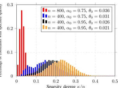
Fig. 2 illustrates the percentage of pattern nodes with the specified sparsity degree defined as%=κ/n, where κis the number of non-zero elements. From the figure we notice two trends: Increasing the sparsity thresholdθ0makes the network
sparser and larger networks become sparser in general.
0 0.1 0.2 0.3 0.4 0.5 0 0.1 0.2 0.3 Sparsity degreeκ/n Percentage of constraints with specified sparsity nn= 400= 800,α0= 0.75,θ0= 0.036 ,α0= 0.75,θ0= 0.031 n= 400,α0= 0.95,θ0= 0.026 n= 400,α0= 0.95,θ0= 0.021
Fig. 2. The percentage of variable nodes with the specified sparsity degree and different values of network sizes and sparsity thresholds. The sparsity degree is defined as%=κ/n, whereκis the number of non-zero elements. C. Recall Phase Results
For the recall phase, in each trial we pick a pattern randomly from the training set, corrupt a given number of its symbols with ±1 noise and use the suggested algorithms to correct the errors. A pattern error is declared if the output does not match the correct pattern. We compare the performance of the two recall algorithms: Winner-Take-All (WTA) and Majority-Voting (MV). Table VII-C shows the simulation parameters in the recall phase for all scenarios (unless specified otherwise).
TABLE I SIMULATION PARAMETERS Parameter ϕ tmax ε η Value 1 20kzk0 0.001 1 0 2 4 6 8 10 0 0.2 0.4 0.6 0.8 1
Number of initial errors
Final patter error rate α0= 0.75,θ0= 0.031 - MV α0= 0.75,θ0= 0.031 - WTA α0= 0.95,θ0= 0.021 - MV α0= 0.95,θ0= 0.021 - WTA
Fig. 3. Pattern error rate against the initial number of erroneous nodes for two different values ofθ0. Here, the network size isn= 400andk= 200. The blue curves correspond to the sparser network (largerθ0) and clearly shows a better performance.
Fig. 3 illustrates the effect of the sparsity thresholdθon the performance of the recall algorithm. Here, we have n= 400
andk= 200. Two different sparsity thresholds are compared together, namely θt∝0.031/t andθt∝0.021/t. Clearly, as network becomes sparser, i.e.θincreases, the performance of both recall algorithms improve.
Fig. 4 illustrates the effect of network size on the perfor-mance of recall algorithms. As obvious from the figure, the performance improves to a great extent when we have a larger network. This is partially because of the fact that in larger networks, the connections are relatively sparser.
Fig. 5 compares the results obtained in simulation with the upper bound derived in Section V. Note that as expected, the bound is quite loose since in deriving inequality (11) we only considered the first iteration of the algorithm.
0 2 4 6 8 10 0 0.2 0.4 0.6 0.8 1
Number of initial errors
Final patter error rate n= 400,α0= 0.75,θ0= 0.031 - MV n= 400,α0= 0.75,θ0= 0.031 - WTA n= 800,α0= 0.95,θ0= 0.029 - MV n= 800,α0= 0.95,θ0= 0.029 - WTA
Fig. 4. Pattern error rate against the initial number of erroneous nodes for two different network sizesn= 800andk= 400. In both casesk=n/2.
0 2 4 6 8 10 0 0.2 0.4 0.6 0.8 1
Number of initial errors
Final patter error rate n= 800- Theory n= 800- Simulation
Fig. 5. Pattern error rate against the initial number of erroneous nodes and comparison with theoretical upper bounds forn= 800,k= 400,α0= 0.95 andθ0= 0.029. 0 1 2 3 4 5 6 0 0.2 0.4 0.6 0.8 1
Number of initial errors
Final patter error rate n= 200, WTA n= 200, MV - Original n= 200, MV - Modified
Fig. 6. Pattern error rate against the initial number of erroneous nodes for two different values ofθ0. Here, the network size isn= 400andk= 200. The blue curves correspond to the sparser network (largerθ0) and clearly show a better performance.
We also investigate the performance of the modified and more practical version of the Majority-Voting algorithm, which was explained in Section IV-B. Fig. 6 compares the perfor-mance of the WTA and original MV algorithms with the modified version of MV algorithm for a network with size n = 200, k = 100 and learning parameters αt ∝ 0.45/t, η= 0.45andθt∝0.015/t. The neural graph of this particular example is rather dense, because of smalln andθ. Here, the modified MV algorithm performs better because of the extra information provided by the `1-norm (compared to the `0
-norm in the original MV algorithm). However, note that we did not observe this trend for the other simulation scenarios where the neural graph was sparser.
Finally, in Fig. 7 we compare perfromance of the proposed method in this paper and the multi-state complex-valued neural networks in [3] and [19]. To have a fair comparison, we first applied the methods of [3] and [19] to a dataset of randomly
0 2 4 6 8 0 0.2 0.4 0.6 0.8 1
Number of initial errors
Final patter error rate C= 50, Subs- [3] C= 50, Rand- [3] C= 100, Rand- [3] C= 400, Subs- [19] C= 400, Rand- [19] C= 2000, Subs- [19] C= 2000, Rand- [19] C= 106, Subs (WTA)
Fig. 7. Recall error rate against the initial number of errors for the method proposed in this paper and those of [3] and [19]. Different pattern retrieval capacities are considered to investigate their effect on the recall error rate.
generated patterns, which is the setting that these methods are designed for, and compared the results to that of our method in its natural setting, i.e. patterns belonging to a subspace. As seen from Fig. 7 the proposed method in this paper could achieve very small recall errors while having a much larger pattern retrieval capacity at the same time.
We then applied the methods of [3] and [19] to the dataset in which patterns belong to a subspace. Interestingly, the performance of the method in [3] deteriorates while that of [19] becomes better in certain cases (e.g. for C = 2000). However, neither of the approaches can achieve the small error rates obtained by the method proposed in this paper. Thus, even though redundancy and structure exists in this particular set of patterns, the mentioned approaches could not exploit it to achieve better pattern retrieval capacities or smaller recall error rates.
VIII. CONCLUSIONS ANDFUTUREWORK
In this paper, we proposed a neural associative memory which is capable of exploiting inherent redundancy in input patterns to enjoy an exponentially large pattern retrieval ca-pacity. Furthermore, the proposed method uses simple iter-ative algorithms for both learning and recall phases which makes gradual learning possible and maintain rather good recall performances. The convergence of the proposed learning algorithm was proved using techniques from stochastic ap-proximation. We also analytically investigated the performance of the recall algorithm by deriving an upper bound on the probability of recall error as a function of input noise. Our simulation results confirms the consistency of the theoretical results with those obtained in practice, for different network sizes and learning/recall parameters.
Improving the error correction capabilities of the proposed network is definitely a subject of our future research. We have already started investigating this issue and proposed a different network structure which reduces the error correction probability by a factor of 10 in many cases [28]. In [29] we proposed a more robust recall algorithms which achieves linear
error correction capabilities.
Extending this method to capture other sorts of redundancy, i.e. other than belonging to a subspace, will be another topic which we would like to explore in future.
Finally, considering some practical modifications to the learning and recall algorithms is of great interest. One good example is simultaneous learn and recall capability, i.e. to have a network which learns a subset of the patterns in the subspace and move immediately to the recall phase. Now during the recall phase, if the network is given a noisy version of the patterns previously memorized, it eliminates the noise. However, if the given pattern is new and had not learned before, the network adjusts the weights in order to learn this pattern as well. Such model is of practical interest and closer to real-world neuronal networks.
ACKNOWLEDGMENT
The authors would like to thank Prof. Wulfram Gerstner and his lab members, as well as Dr. Amin Karbasi for their helpful comments and discussions. This work was supported by Grant 228021-ECCSciEng of the European Research Council.
APPENDIXA
AVERAGE NEIGHBORHOOD SIZE
In this appendix, we find an expression for the average neighborhood size for erroneous nodes,St=E(|N(Et)|). To this end, we assume the following procedure for constructing a right-irregular bipartite graph:
• In each iteration, we pick a variable node xwith a de-gree randomly determined according to the given dede-gree distribution.
• Based on the given degree dx, we pick dx constraint nodes uniformly at randomwith replacementand connect xto the constraint node.
• We repeat this process n times, until all variable nodes are connected.
Note that the assumption that we do the process with replace-ment is made to simplify the analysis.
Now we are interested in finding the average number of constraint nodes in each round of the above procedure. With some abuse of notations, letSedenote the number of constraint nodes connected to pattern nodes in round e. We write Se recursively in terms ofeas follows:
Se+1 = Edx( dx X j=0 d x j Se m dx−j 1−Se m j (Se+j)) = Edx(Se+dx(1−Se/m)) = Se+ ¯d(1−Se/m), (16)
where d¯ = Edx(dx) is the average degree of the pattern
nodes. In words, the first line calculates the average growth of the neighborhood when a new variable node is added to the graph. The proceeding equalities follows from relationships on binomial sums. Noting thatS1= ¯d, one obtains:
St=m 1−(1− d¯ m) |Et| (17)
In order to verify the correctness of the above analysis, we have performed some simulations for different network sizes and degree distributions obtained from the graphs returned by the learning algorithm. We generated2000random graphs and calculated the average neighborhood size in each iteration. The result forn= 200,m= 100 is shown in Figure 8, where the average neighborhood size in each iteration is illustrated and compared with theoretical estimations given by equation (17). From the figure, it is obvious that the theoretical value is a very good approximation of the simulation results.
0 40 80 120 160 200 0 20 40 60 80 100 Construction round (t) St Theorey Simulation
Fig. 8. The theoretical estimation and simulation results for the average neighborhood size of irregular graphs with a given degree-distribution for
n= 200,m= 100and over2000random graphs.
REFERENCES
[1] J. J. Hopfield, “Neural networks and physical systems with emergent collective computational abilities,”Proc. Natl. Acad. Sci. U.S.A., vol. 79, no. 8, pp. 2554–2558, 1982.
[2] S. S. Venkatesh and D. Psaltis, “Linear and logarithmic capacities in associative neural networks,”IEEE Trans. Inf. Theor., vol. 35, no. 3, pp. 558–568, Sep. 1989.
[3] S. Jankowski, A. Lozowski, and J. M. Zurada, “Complex-valued mul-tistate neural associative memory.”IEEE Trans. Neural Netw. Learning Syst., vol. 7, no. 6, pp. 1491–1496, 1996.
[4] M. K. Muezzinoglu, C. Guzelis, and J. M. Zurada, “A new design method for the complex-valued multistate hopfield associative memory,” IEEE Trans. Neur. Netw., vol. 14, no. 4, pp. 891–899, Jul. 2003. [5] A. H. Salavati, K. R. Kumar, M. A. Shokrollahi, and W. Gerstnery,
“Neural pre-coding increases the pattern retrieval capacity of hopfield and bidirectional associative memories,” inProc. IEEE Int. Symp. Inf. Theor. (ISIT), 2011, pp. 850–854.
[6] V. Gripon and C. Berrou, “Sparse neural networks with large learning diversity,”IEEE Trans. Neur. Netw., vol. 22, no. 7, pp. 1087–1096, 2011. [7] T. Richardson and R. Urbanke,Modern Coding Theory. New York,
NY, USA: Cambridge University Press, 2008.
[8] C. E. Shannon, “A mathematical theory of communication,”Bell system technical journal, vol. 27, no. 379, pp. 948–958, 1948.
[9] R. J. McEliece, E. C. Posner, E. R. Rodemich, and S. S. Venkatesh, “The capacity of the hopfield associative memory,”IEEE Trans. Inf. Theor., vol. 33, no. 4, pp. 461–482, Jul. 1987.
[10] K. R. Kumar, A. H. Salavati, and M. A. Shokrollahi, “Exponential pattern retrieval capacity with non-binary associative memory,” inIEEE Inf. Theor. workshop (ITW), Oct 2011, pp. 80–84.
[11] S. Hoory, N. Linial, A. Wigderson, and A. Overview, “Expander graphs and their applications,”Bull. Amer. Math. Soc., vol. 43, no. 4, pp. 439– 561, 2006.
[12] K. Pagiamtzis and A. Sheikholeslami, “Content-addressable memory (cam) circuits and architectures: A tutorial and survey,”IEEE Journal of Solid-State Circuits, vol. 41, no. 3, pp. 712–727, 2006.
[13] J. Chen, H. Guo, W. Wu, and W. Wang, “imecho: an associative memory based desktop search system,” in Proc. ACM Conf. Information and knowledge management, 2009, pp. 731–740.
[14] D. O. Hebb, The Organization of Behavior: A Neuropsychological Theory. New York: Wiley&Sons, 1949.
[15] D. J. Amit, H. Gutfreund, and H. Sompolinsky, “Storing infinite numbers of patterns in a spin-glass model of neural networks,”Phys. Rev. Lett., vol. 55, pp. 1530–1533, Sep 1985.
[16] J. Hertz, R. G. Palmer, and A. S. Krogh,Introduction to the Theory of Neural Computation, 1st ed. Boston, MA, USA: Addison-Wesley Longman Publishing Co., Inc., 1991.
[17] J. Koml´os and R. Paturi, “Effect of connectivity in an associative memory model,” J. Comput. Syst. Sci., vol. 47, no. 2, pp. 350–373, 1993.
[18] J. J. Hopfield, “Neurons with graded response have collective computa-tional properties like those of two-state neurons,”Proc. Natl. Acad. Sci. U.S.A., vol. 81, no. 10, pp. 3088–3092, 1984.
[19] D.-L. Lee, “Improvements of complex-valued Hopfield associative mem-ory by using generalized projection rules.”IEEE Trans. Neural Netw., vol. 17, no. 5, pp. 1341–1347, 2006.
[20] C. Berrou and V. Gripon, “Coded Hopfield networks,” in Int. Symp. Turbo Codes & Iterative Info. Processing (ISTC), Sep 2010, pp. 1–5. [21] R. H. Gold, “Optimal binary sequences for spread spectrum
multiplex-ing,”IEEE Trans. Inf. Theor., vol. 13, no. 4, pp. 619–621, Sep. 1967. [22] S. S. Venkatesh, “Connectivity versus capacity in the hebb rule,” in
Theoretical Advances in Neural Computation and Learning. Springer, 1994, pp. 173–240.
[23] P. Peretto and J. J. Niez, “Long term memory storage capacity of multiconnected neural networks,”Biol. Cybern., vol. 54, no. 1, pp. 53– 64, 1986.
[24] B. Kosko, “Bidirectional associative memories,” Systems, Man and Cybernetics, IEEE Transactions on, vol. 18, no. 1, pp. 49–60, 1988. [25] T. Kohonen, “Self-organized formation of topologically correct feature
maps,”Biological cybernetics, vol. 43, no. 1, pp. 59–69, 1982. [26] P. Tavan, H. Grubm¨uller, and H. K¨uhnel, “Self-organization of
associa-tive memory and pattern classification: recurrent signal processing on topological feature maps,”Bio. cyber., vol. 64, no. 2, pp. 95–105, 1990. [27] S. Chartier, G. Giguere, D. Langlois, and R. Sioufi, “Bidirectional asso-ciative memories, self-organizing maps and k-winners-take-all: uniting feature extraction and topological principles,” inInt. Joint Conf. Neur. Net. (IJCNN), 2009, pp. 503–510.
[28] A. H. Salavati and A. Karbasi, “Multi-level error-resilient neural net-works,” inProc. Int. Symp. Inf. Theor. (ISIT), 2012, pp. 1064–1068. [29] A. Karbasi, A. H. Salavati, and A. Shokrollahi, “Iterative learning and
denoising in convolutional neural associative memories,” in Proc. Int. Conf. on Machine Learning (ICML), ser. ICML ’13, Jun. 2013, to appear. [30] L. Xu, A. Krzyzak, and E. Oja, “Neural nets for dual subspace pattern recognition method,”Int. J. Neur. Syst., vol. 2, no. 3, pp. 169–184, 1991. [31] E. Oja and T. Kohonen, “The subspace learning algorithm as a formalism for pattern recognition and neural networks,” inIEEE Int. Conf. Neur. Netw., vol. 1, Jul 1988, pp. 277–284.
[32] E. J. Cand`es and T. Tao, “Near-optimal signal recovery from random projections: Universal encoding strategies?”IEEE Trans. Inform. Theor., vol. 52, no. 12, pp. 5406–5425, 2006.
[33] D. L. Donoho, A. Maleki, and A. Montanari, “Message-passing algo-rithms for compressed sensing,”Proc. Nat. Acad. Sci. U.S.A., vol. 106, no. 45, pp. 18 914–18 919, 2009.
[34] J. A. Tropp and S. J. Wright, “Computational methods for sparse solution of linear inverse problems,”Proceedings of the IEEE, vol. 98, no. 6, pp. 948–958, 2010.
[35] E. Oja and J. Karhunen, “On stochastic approximation of the eigen-vectors and eigenvalues of the expectation of a random matrix,”Math. Analysis and Applications, vol. 106, pp. 69–84, 1985.
[36] L. Bottou, “Online algorithms and stochastic approximations,” inOnline Learning and Neural Networks, D. Saad, Ed. Cambridge Univ. Press, 1998.
[37] M. Sipser and D. A. Spielman, “Expander codes,” IEEE Trans. Inf. Theor., vol. 42, pp. 1710–1722, 1996.
[38] S. Jafarpour, W. Xu, B. Hassibi, and A. R. Calderbank, “Efficient and robust compressed sensing using optimized expander graphs,” IEEE Trans. Inf. Theory, vol. 55, no. 9, pp. 4299–4308, 2009.
[39] K. R. Kumar, A. H. Salavati, and M. A. Shokrollahi, “A non-binary associative memory with exponential pattern retrieval capacity and iterative learning,” http://arxiv.org/abs/1302.1156, Ecole Polytechnique Federale de Lausanne (EPFL), Tech. Rep., Feb. 2013.

![Fig. 7. Recall error rate against the initial number of errors for the method proposed in this paper and those of [3] and [19]](https://thumb-us.123doks.com/thumbv2/123dok_us/9674343.2848975/12.918.82.458.79.358/recall-error-initial-number-errors-method-proposed-paper.webp)

