The wild bootstrap resampling in regression imputation algorithm with a Gaussian Mixture Model

Imputation Algorithm with a Gaussian Mixture Model

Aisyah Mat Jasin 1_{, Daniel Neagu}1 _{and Attila Csenki} 1 1 _{University of Bradford, Bradford BD7 1DP, UK}

[email protected] [email protected] [email protected]

Abstract. Unsupervised learning of finite Gaussian mixture model (FGMM) is used to learn the distribution of population data. This paper proposes the use of the wild bootstrapping to create the variability of the imputed data in single miss-ing data imputation. We compare the performance and accuracy of the proposed method in single imputation and multiple imputation from the R-package Amelia II using RMSE, R-squared, MAE and MAPE. The proposed method shows better performance when compared with the multiple imputation (MI) which is indeed known as the golden method of missing data imputation techniques.

Keywords: Missing Data Imputation, Gaussian Mixture Model, Bootstrap.

1

Introduction

Missing data can occur in data records for various reasons, such as: data entry errors, system failures, or respondents who avoid answering questions within a survey. Vari-ous methods have been proposed to deal with the missing data problem. The standard technique is discarding observations or variables that contain missing values. The de-letion method is inappropriate when the missing proportions are high, resulting in inef-ficient parameter estimates, and estimated results tend to be underestimated. To deal with these issues, imputation methods can be used to substitute missing values with plausible values. For example, the single mean imputation consists of replacing the missing values with the mean, median or mode value. However, this simple approach produces biased analysis results. The multiple imputation method introduced in [1] is a complex approach where missing data are filled-in by drawing multiple sets of plete data that contain different plausible values. This method is complicated and com-putationally expensive [2], especially for large data sets because execution processes are implemented through three phases in several iterations. The improved version of the single imputation technique such as conditional mean imputation, which incorpo-rates the statistical and machine learning methods with multivariate Gaussian mixture models (GMM)[3] have gained interest in many years[4].

The conditional mean imputation (also known as ordinary least square, OLS) or re-gression imputation can preserve the data distribution, according to Di Zio [5]. The

conventional OLS ₀ 1 ˆ_i J _{j j i} j y   x  

 



 implementation requires the use of random error



_i which can be obtained in two ways [6]: 1) draw a random error with underlying assumption that it is independent and identically distributed, that follows a Gaussian distribution with zero mean and finite variance; 2) draw a random error with replace-ment from the empirical distribution of the estimated residuals



_i

 

y

_i

y

ˆ

_i[7]. Problems can occur in the random error and residual



i in method (1) that will create the sparsity

problem whereas the random



_i generation will be either too large or too small although the normality distribution assumption is met. The sparsity of data in method (2) will be inconsistent if the data distribution has different clusterings and each cluster consists of a different density. The sparsity of data creates some problems such as increases in the variance between the imputed and original data.

The conditional mean imputation proposed in [5] does not consider adding the re-siduals. Although this method may preserve the data distribution, it will underestimate the variability, introduce the bias on imputed data and the result of imputed data will be highly inaccurate. The additional steps are required to improve data sparsity in the random error



_i generated in the OLS to obtain a better predicted missing value.

The main objective of this study is to investigate the random error and employ the wild bootstrap [8] [9] on the missing data prediction using regression imputation on the Gaussian mixture model. The wild bootstrap is used to improve the variance in hetero-scedasticity issue when the data variance is not homoscedastic [8][9]. Further details about the wild bootstrap approach are discussed in the next section that introduces the modelling framework.

In this paper, we employ the wild bootstrap to the single imputation technique in missing value prediction, since the GMM framework is flexible to learn multimodal data distribution. We combine the GMM model with the proposed missing data predic-tion method. We also employ the wild bootstrap to investigate the effect of the sparsity of imputed data in a different mixture data distribution case. Thus, we would like to show that the performance of single imputation may perform well, and as good as the implementation of MI. We assume that the data is missing data at random (MAR).

This paper is organized as follows: in Section 2, we present the Gaussian mixture model framework and the proposed regression imputation with wild bootstrap tech-nique. In Section 3 we discuss the experimental evaluation and experimental results. Section 4 concludes the paper and identifies further directions for research and study.

2

Modelling Framework

GMM is a powerful probabilistic model used in predicting specifically in data cluster-ing [5]. This model is flexible to learn from different data distributions by fittcluster-ing the probability density function (PDF) to represent different clusters [3]. The well-known

strategy for finding the Maximum Likelihood (ML) parameter estimation uses the Ex-pectation-Maximization (EM) algorithm [10]. GMM applications to missing data prob-lems have been studied extensively for example in [4][5][11].

2.1 Definitions

Suppose the data setX having

N

units of independent and identically distributed (i.i.d) data points with

p

-column vectors can be written as follows:

Observa-tion (index)

X

1

X

2

..

X

l

..

X

p

1

11 O

x

x

₁₂O

..

x

₁O_l

..

x

₁O_p

..

:

:

..

..

..

:

1

n

11 O n

x

12 O n

x

..

1 O n l

x

..

1 O n p

x

1

1

n



1 ( 1)1 M n

x

_ 1 ( 1) 2 M n

x

_

..

NA

..

1 ( 1) M n p

x

_

:

:

:

..

..

:

N

1 M N

x

x

_NM₂

..

NA

..

x

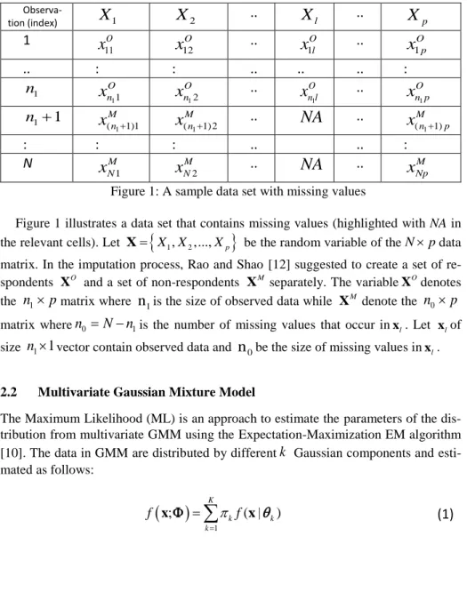
M_Np

Figure 1: A sample data set with missing values

Figure 1 illustrates a data set that contains missing values (highlighted with NA in the relevant cells). Let X



X X₁, ₂,...,X_p



be the random variable of theNpdata matrix. In the imputation process, Rao and Shao [12] suggested to create a set of re-spondents _XO _{and a set of non-respondents X}M_{separately. The variableX}O_denotes the

n

₁



p

matrix where

n

₁is the size of observed data while XMdenote the

n

₀



p

matrix where

n

₀

 

N

n

₁is the number of missing values that occur inx_l. Let x_lof size

n

1



1

vector contain observed data and

n

0be the size of missing values inxl. 2.2 Multivariate Gaussian Mixture Model

The Maximum Likelihood (ML) is an approach to estimate the parameters of the dis-tribution from multivariate GMM using the Expectation-Maximization EM algorithm [10]. The data in GMM are distributed by different

k

Gaussian components and esti-mated as follows:





1

;

( |

)

K k k k

f



f







x



x



(1)

where

f x

( |



_k

)

is the density of p-variate Gaussian distribution with the

k

compo-nent. The vector  contains the full set of parameters in the mixture model

1 1

( ,...,





_K

; ,...,

_K

)









, where



_k is the vector of unknown parameters of mean vec-tor



_kand covariance matrix



_k.

The mixing coefficients (or weights)



_kfor the kthcomponent must satisfy the con-ditions 0



_k 1, and



Kk₁



k



1

. The GMM is a dynamic model where it is not

required to specify any column vector to be an input or output particularly.

2.3 The General EM Algorithm

The EM algorithm is a statistical tool to find the maximum likelihood estimates of the set parameters such as mean, variances, covariances and regression coefficients of a model. The optimisation algorithm introduced by Dempster, Laird, and Rubin [10] starts with an initial estimate of  and iteratively executes the process until it satisfies the convergence criteria. The iterative process has two steps known as the E-step and the M-step. The E-step computes the probability membership



ikfor all data points xi of mixture component

k

. The M-step will update the value of the parameter with respect to the

k

Gaussian component. Let denote q as an iteration counter, the expected values of the posterior distribution are computed by:

( ) 1 ˆ ˆ ( |ˆ , ) ˆ ˆ ˆ ( |ˆ , ) o q k i k k ik K o j i j j j f f







 



x x    

(2)

In the M-step, we use the expected values in the posterior distribution (2) to re-esti-mate the means, covariances and mixing coefficients. The new set of parameters

(q1)

 are updated as follows: ( 1) ˆq k k N N



 _

for k=1,…,K,

(3)

𝜇̂_𝑘(𝑞+1)= 1 𝑁𝑘 ∑ 𝜏𝑖𝑘𝐱̂𝑖𝑘 𝑁 𝑖=1

(4)

( 1) 1 1 ˆ q N _{[(ˆ )(ˆ )}T ˆMM_] k ik ik k ik k ik i k N    



x  x      

₍₅₎

2.4 The Least Square Method

The conditional mean imputation is also known as regression imputation [13]. The im-puted values are regressed from independent variables X_p. Let consider the following linear regression model:

0 1

il i i

x  

 

x 



,

i1, 2,...,n (6)

where the response variable xil is predicted from regression coefficients



0 and



1 with random error εi~N(0,σ2) i.i.d. and uncorrelated. The matrix development of

equa-tion (6) is presented as follows:

1 : , l l Nl x x           x 11 1 1 1 ... : : ... : , 1 ... p N Np x x x x            X 1 : , p              1 : N





          

In general, xlis an

N



1

vector of the dependent variable contains missing values, Xis a Np matrix of observed variables, is ap1 vector of the regression coeffi-cients and



is a N1vector of random errors. The general least square estimator of

 based on observed values is:





1 ˆO T T l   X X X X  (7)

In the presence of missing data, the imputed values are obtained by the conditional mean imputation technique which corresponds to imputed values generated from a set of regression equation calculated in (7) as discussed in [14][13]. There are two ways to generate the random error component _i. The random error component _i can be gen-erated either with εi~N(0,σ2) or residual.

2.5 Fundamentals of the Bootstrap Method

The bootstrap non-parametric resampling technique was proposed by Efron [15] for estimating a standard error , confidence interval in various types of distributions. This method was extended in [16] and [17] to generate the random error



_iin the regression

model. Let





1

1, 2,..., n



X x x x is a random sample from p-variate normal distribution K where n1refers to the size of observed data

O

X as shown in Figure 1. Let _X(bk)_denote the bootstrap resampled data generated by sampling with replacement from the original dataset Xk where bindicates the counter b1,...,B of drawing samples of bootstrap and k refers to the current Gaussian component. In this study, the resampling and pa-rameter estimation are implemented on the observed data O

k

X where the superscript O refers to observed data.

2.6 The Wild Bootstrap

Wu [8] introduced the wild bootstrap to deal with the heteroscedasticity issue. Later, a better approximation of the wild bootstrap was proposed by Liu [9]. The wild bootstrap is based on the modification of the bootstrap residual approach of the least square esti-mation. Wu [8] improved the resampling residual with replacement in bootstrap by drawing a value of *

i

t that follow a standard normal distribution with zero mean and unit variance: * ˆ ˆ 1 b T i il i i i x x t w



    (8)

wherew_i xT_i (X XT )x_i. However, the error variance *_ˆ i i

t are inconsistent. There-fore, authors in [18] proposed to compute *

i

t by drawing a sample aiwith replacement:

1 * 1 2 1 ₁ ˆ ˆ ˆ ˆ ( ) k i i i i _n k _i i t a n

 

 

     



(9) where 1 1 1 1 ˆ nk ˆ k i i n     



.

The second wild bootstrap technique employed in this study is the Liu’s bootstrap [9]. Liu [9] proposed *

i

t in Wu [8] by resampling a set of central residual with zero mean and unit variance that has third central moments equal to one. Liu proposed two procedures to draw random numbers *

i

t . However, we consider the second procedure as it is appropriate for normal distribution. Liu’s bootstrap is conducted by drawing random numbers:

1 2 ( 1) ( 2) i

t D D E D E D (10)

where D₁and D₂are random i.i.d that follows normal distribution with means 0.5* ( 17 / 6 1 / 6) and 0.5* ( 17 / 6 1 / 6)respectively, and variance 0.5. 2.7 The Non-Parametric Wild Bootstrap Applied in Missing Data Imputation The bootstrap procedure based on the resample approach in the GMM is described in the following steps:

1. Initiate the set of parameters with K-means algorithm. 2. Compute the residual for each Gaussian component:

a. Fit Gaussian mixture model using the parameter values from the step 1. b. Compute the residual: 𝜀̂𝑘= 𝐗𝑙𝑘𝛃̂𝑘where k is the Gaussian component k

= 1,..,K. 3. For b = 1,.., B

a. Draw a vector 𝜀̂𝑘of n1k i.i.d sample with a simple random sampling with replacement. The vector 𝜀̂𝑘is generated from step 2b with respect to the

option of the Wu’s [8] or Liu’s[9] bootstrap procedure as discussed in the Section 2.6.

b. Fit Gaussian mixture model using the parameter values from the step 1. c. In the E-step,

i. Compute the posterior probabilities vector



_ikin equation (2) on the observed data.

d. In the M-step,

i. Impute the missing values of size n₀k using a linear regression model (6) based on OLS estimator ˆ(Ok) _{in (12):}

ˆ0( ) ˆ1( ) *ˆ / 1

k k

O O

il i i i i

x 







x t



w where the residual *

i

t taken from the step 3a.

ii. Update the new parameter  for each component in GMM as shown in (3), (4) and (5).

3

Experiments and Discussion of Results

In this section, the numerical results are presented on real and simulated datasets.

3.1 The Non-Parametric Wild Bootstrap Applied in Missing Data Imputation Dataset: We applied various evaluation criteria on one real dataset and one artificial dataset with two variables and two Gaussian classes. The first case study is the Old Faithful Geyser dataset [19]. This dataset contains 272 records on the waiting time be-tween geyser eruptions (waiting) and the duration of eruptions (eruptions) in Yellow-stone National Park, USA.

For the artificial case study, the values are randomly sampled with 1000 observations of two Gaussian classes with different position mean values and positive-negative cor-relation. Data are drawn with normal distribution using the following parameters:

1 0.5  

,

 2 0.5 ' 1 (4, 2)  

,

' 2 ( 2, 6)    1 1 0.7 0.7 1     _   

,

1 3 0.9 0.9 3       

Software: the proposed method in these experiments were conducted using Matlab version 2017a. The proposed method is compared with multiple imputation available in the R-package Amelia II. The comparisons are conducted based on the artificial missing data generated with different missing data percentages (MDP): 5%, 10%, 15% and 20%.

Imputation implementation: the missing data are imputed based on the regression imputation. Prior to the imputation process, the K-means algorithm is used to determine

initial parameter values of mixing proportion



_k, mean



_kand covariance matrix



_k in GMM. The stopping criteria is based on a selected threshold where the different iterations were less than 106.

Evaluation criteria: These experiments are designed to measure the performance and prediction accuracy between predicted and actual values. RMSE computes the devia-tion between predicted and actual values that employed by most missing data imputa-tion studies. The greater the deviaimputa-tion means the greater variance between them. There-fore, the lower value shows better performance:

2 1

(

ˆ

)

N i i i

y

y

RMSE

N









(11)

MAPE was used to measure the average relative error of the imputation accuracy:

1

ˆ

100

N _{i i} i i

y

y

MAPE

N



y









(12)

MAE was used to measure the average error of each different in imputation:

1

1

ˆ

N i i i

MAE

y

y

N



 





(13)

R-squared values were used to describe the variance in goodness-of-fit for the re-gression models between observed data and the expected values of the dependent vari-able. The range of R-squared is between 0 and 1:

2 2 1 2 1

ˆ

(

)

(

)

n i i i n i i

y

y

R

y

y

 











(14) 3.2 Experimental results

In this study, we compare the imputation accuracy using MAPE and MAE whilst meas-uring the performance using RMSE and R-Squared of three methods: single regression imputation combined with Wu’s and Liu’s wild bootstrap and MI. The better results are highlighted in bold font.

Table 1 summarizes the performance and prediction accuracy of the three methods on the Old Faithful Geyser dataset while Table 2 shows the result estimation on the random data generation. The result of the proposed methods in RMSE shows better performance and significantly different between the MI with the proposed Wu’s and Liu’s method in all MDP proportions. This is shown in the 5% MDP, Wu and Liu method yielded 7.8225 and 7.8879 respectively while MI gained 9.8719. It is also found in 10%, 15% and 20% MDP where the Wu's and Liu's method have outperformed the MI where the result of Wu's shows 7.0955, 6.6819 and 6.7349 while Liu shows 7.8746, 7.0150 and 7.2354 in RMSE. In contrast, the MI obtained 8.4187, 8.7004 and 8.9103 higher than Wu's and Liu's method in 10%, 15% and 20% MDP respectively.

The R-squared values are used to quantify the overall model performance of variance in response variable explained by the independent variables. The larger the R-squared means the more variability is explained by the linear regression model. The result of R-squared presented in Table 1 showed that the proposed method gives the best perfor-mance with 0.6338% for 5% of MDP proportion followed by 0.6836, 0.7683 and 0.7127 for Wu, while Liu’s obtained 0.6894, 0.6869 and 0.7050 for the 10%, 15% and 20% of MDP respectively on the Faithful data set. The R-squared obtained by the pro-posed method in the random generation data in the Table 2 showed less than 0.6% for all MDP percentages. In contrast, the MI in Amelia gives a lower variance than the proposed method in all MDP proportions with R-squared ranging from 0.03 to 0.2.

The imputation accuracy is measured based on the average relative error between predicted missing data and the original data using mean absolute percentage error (MAPE) and mean absolute error (MAE).

The result of MAE in the Table 1 showed that the Wu’s and Liu’s methods are con-sistently outperformed the MI method on the Old Faithful Geyser dataset. In contrast, in the Table 2, the Liu’s method offered consistent and better accuracy than MI method. Meanwhile the Wu’s method showed inconsistent improvement in the measure of av-erage error magnitude to MI method on the random data generation.

As can be observed from the MAPE values obtained in Table 1, the proposed method of Wu’s and Liu’s performed better imputation on the Old Faithful Geyser data set. Meanwhile, by observing the MAPE values gained in the Table 2, Liu’ method showed consistent to defeat the MI method compared to Wu’s method.

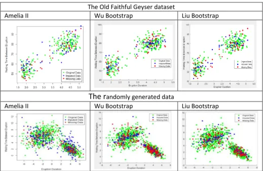
A plot of the result shown in Figure 1 compare the outcome between multiple im-putation technique in r-package Amelia II and the proposed methods.

Table 1. The MAPE, MAE, R-square and RMSE estimates on the Old Faithful Geyser dataset MAPE MAE R square RMSE 5% Amelia _Wu 0.6220 _0.2758 6.5928 _2.6453 0.4960 _0.6338 9.8719 _7.8225 Liu 0.1713 1.7281 0.4212 7.8879 10% Amelia 0.0827 1.5636 0.6450 8.4187 Wu 0.0379 0.6959 0.6836 7.0955 Liu 0.0190 0.3594 0.6894 7.8746 15% Amelia _Wu 0.0346 _0.0012 1.0379 _0.0342 0.5184 _0.7683 8.7004 _6.6819 Liu 0.0167 0.5018 0.6869 7.0150 20% Amelia _Wu 0.0432 _0.0054 1.6841 _0.2144 0.4959 _0.7127 8.9103 _6.7349 Liu 0.0104 0.3994 0.7050 7.2354

Table 2. The MAPE, MAE, R-square and RMSE estimates on the randomly generated data

MAPE MAE R square RMSE 5% Amelia _Wu 1.5798 _0.0469 0.7748 _0.1055 0.2439 _0.2593 2.0230 _1.8642 Liu 0.0721 0.1604 0.3754 1.8066 10% Amelia _Wu 0.1259 _0.1344 0.1477 _0.5811 0.2206 _0.3977 2.2926 _2.1557 Liu 0.0089 0.0377 0.5803 1.6889 15% Amelia _Wu 0.1674 _0.0272 0.3105 _0.1812 0.0272 _0.1316 2.2817 _2.3463 Liu 0.0203 0.1282 0.5197 1.7214 20% Amelia _Wu 0.0501 _0.0435 0.1159 _0.3528 0.1206 _0.1954 2.7461 _2.1858 Liu 0.0127 0.1070 0.4586 1.8340

The Old Faithful Geyser dataset

Amelia II Wu Bootstrap Liu Bootstrap

The r

andomly generated data

Amelia II Wu Bootstrap Liu Bootstrap

Fig. 1. The scatter plot of two datasets using R Amelia II and the proposed methods

4

Conclusions

In this paper, we proposed a method for single imputation that incorporates wild boot-strap in order to create the variability of imputed data as for example Multiple Imputa-tion (MI) does. The MI is indeed known to be the preferred method in handling missing data problems over the years compared to the single imputation methods.

The imputation process in MI involves several steps while single imputation has simpler implementation compared to MI. The missing data in MI are imputed for M times with different plausible values and combine appropriately in the analysis stage. The sparsity of imputed data is a matter of concern because it will reflect the variance and measurement error between predicted and original data. Thus, the main purpose of this comparison is to show that the performance of single imputation in the Gaussian mixture model may perform well and as good as the implementation of MI.

The performance of this method is measured by the RMSE, R-squared, MAE, and MAPE. Based on the results, we summarize that the single missing data imputation combined with the wild bootstrap is preferrable over the MI technique for the data con-taining several Gaussian distributions. Furthermore, the imputation process on the Gaussian mixture model could be relevant to preserve the originality of data distribu-tion.

Since this study is implemented on bivariate data with two Gaussian components, in the future work we will focus on multivariate data with multiple Gaussian components.

References

[1] D. B. Rubin, “Multiple imputations in sample surveys - A phenomenological Bayesian approach to nonresponse,” in Proceedings of the Survey Research Methods Section of

the American Statistical Association, pp. 20–34(1978).

[2] J. Honaker, G. King, and M. Blackwell, “Amelia II: A program for missing data,” J.

Stat. Softw. 45(7), 47(2006).

[3] G. McLachlan and D. Peel, Finite Mixture Models. Wiley, New York(2000).

[4] Z. Ghahramani and M. I. Jordan, “Supervised Learning from Incomplete Data via an EM Approach,” in Advances in Neural Information Processing Systems.6,120– 127(1994).

[5] M. Di Zio, G. Ugo, and O. Luzi, “Imputation through finite Gaussian mixture models,”

Comput. Stat. Data Anal. 51(11), 5305–5316(2007).

[6] M. Paik, “Fractional Imputation,”(Unpublished Doctoral Thesis),Iowa State University,USA (2009).

[7] M. S. Srivastava and M. Dolatabadi, “Multiple imputation and other resampling schemes for imputing missing observations,” J. Multivar. Anal. 100(9),1919–1937 (2009).

[8] C. F. J. Wu, “Jackknife, Bootstrap and Other Resampling Methods in Regression Analysis,” Ann. Stat. 14(4), 1261–1295(1986).

[9] R. Y. Liu, “Bootstrap procedures under some non-i.i.d. models,” Ann. Stat.16(4),1696– 1708(1988).

[10] A. P. Dempster, A. P. Dempster, N. M. Laird, N. M. Laird, D. B. Rubin, and D. B. Rubin, “Maximum likelihood from incomplete data via the EM algorithm,” J. R. Stat.

Soc. Ser. B, 39(1),1–38(1977).

[11] E. Eirola, A. Lendasse, V. Vandewalle, and C. Biernacki, “Mixture of Gaussians for distance estimation with missing data,” Neurocomputing, 131, 32–42(2014).

[12] J. S. J.N.K. Rao, “Jackknife Variance Estimation with Survey Data Under Hot Deck Imputation,” Biometrika Trust, 79(4),811–822(1992).

[13] C. K. Enders, Applied missing data analysis.The Guilford Press,New York(2010). [14] C. R. Harvey, “The specification of conditional expectations,” J. Empir. Financ., 8(5),

573–637(2001).

[15] B. Efron, “Bootstrap Methods : Another Look at the Jackknife,” Ann. Stat.7(1),1–26 (1979).

[16] E. Hardle, W. and Mammen, “Comparing Nonparametric versus Parametric Regression Fits,” Ann. Stat.21,1926–1947(1993).

[17] M. Zadkarami, “Bootsrapping: A Nonparametric Approach to Identify the Effect of Sparsity of Data in the Binary Regression Models,” J. Appl. Sci.8(17), 2991–2997 (2008).

[18] F. Cribari-Neto and S. G. Zarkos, “Bootstrap methods for heteroskedastic regression models: evidence on estimation and testing,” Econom. Rev.18(2), 211–228(1999). [19] A. Azzalini and A. W. Bowman, “A Look at Some Data on the Old Faithful Geyser,” J.

Appendix A: The notation list.

X An entire random sample of size N and p-column.

O

X The observed values of random vector X

M

X The p-feature vectorsXcontains missing values

oc-cur in Xl

1

n

The number of observed data in O

X

0

n

The number of missing data in M

X

K Total number Gaussian of components

k

 Parameter theta that consists of parameter mean

vector kand covariance matrix k k

 The mean vector

k

 The covariance matrix

 Mixing proportion of the current Gaussian

compo-nent

0k1, The probability of mixing coefficient must be

be-tween 0 and 1.

1 1

K k k 



The sum of mixing coefficient of each component

must be equal to one

1 1

( ,...,





_K; ,..., _K)

 





_{The vector}  containing the set of parameters



K

and



K



;



f x The mixture density containing all the parameters of

mixture model ( | k)

f x  The mixture of density function of vector X

condi-tioned on parameter estimation theta.





1 ; ( | ) K k k k f  f    



x x The probability density function governed by the set _{of parameters mixing coefficient and theta with}

K-component mixture density

ik



The posterior probability or responsibility for each

data point that belongs to the th

k component

0

 Beta 0 is represented as the intercept of regression

coefficient

₁ Beta 1 is represented as the slope of regression

0 1

il i i

x   x  The ordinary leas square model (OLS)





1

ˆO T T

l



 X X X X

 The least square estimator of _ˆO

εi~N(0,σ2) The random error component follows he normal

dis-tribution with mean 0 and variance

(bk)

X The sample data after bootstrapping

O k

X The observed data based on the k current Gaussian

component

1,...,

b B b is a counter value for bootstrap iterative process

until B times

* i

t The non-parametric bootstrap resampled residual

ˆ

_i

x

_il

x

ˆ

_il



 

( )

T T

i i i

w x X X x _{The leverage is the} th

i

diagonal element of Hat Ma-trix 1 1 2 1 1 ˆ ˆ ˆ ˆ ( ) k i i i _n k i i a n         



The non-parametric bootstrap resampled residual proposed to improve the random draw of Wu’s algo-rithm

1

Dand D2 The i.i.d that follows normal distribution

1k O n

X _{The observed data of}

n

₁ size and k Gaussian

compo-nent

𝜀̂𝑖= 𝑥𝑖𝑙− 𝑥̂𝑖𝑙 The estimated residual fitted by OLS model