Research
Paper Volume-4, Issue-2 E-ISSN: 2347-2693
An Algorithm for Mining Frequent Closed Itemsets with Density
from Data Streams
Caiyan Dai
1and Ling Chen
2*
1
College of Computer Science and Technology, Nanjing University of Aeronautics and Astronautics, China,
2*
Department of Computer Science, Yangzhou University, China
www.ijcseonline.org
Received: Jan /23/2016 Revised: Feb/04/2016 Accepted: Feb/18/2016 Accepted: Feb/29/2016
Abstract—Mining frequent closed itemsets from data streams is an important topic. In this paper,we propose an algorithm for
mining frequent closed itemsets from data streams based on a time fading module. By dynamically constructing a pattern tree, the algorithm calculates densities of the itemsets in the pattern tree using a fading factor. The algorithm deletes real infrequent itemsets from the pattern tree so as to reduce the memory cost. A density threshold function is designed in order to identify the real infrequent itemsets which should be deleted. Using such density threshold function, deleting the infrequent itemsets will not affect the result of frequent itemset detecting. The algorithm modifies the pattern tree and detects the frequent closed itemsets in a fixed time interval so as to reduce the computation time. We also analyze the error caused by deleting the infrequent itemsets. The experimental results indicate that our algorithm can get higher accuracy results, needs less memory and computation time than other algorithm
Keywords—data streams; frequent closed itemsets; data mining; time fading model
I. INTRODUCTION
Today, tremendous amounts of data and potentially infinite volumes of data streams are generated in many applications such as network intrusion detection, financial transaction flows, telephone call records, sensor streams, and meteorological data. Unlike the finite, statically stored data sets, a data stream is massive, continuous, temporally ordered, dynamically changing, and potentially infinite. A typical example of stream data is the trading of public securities in the United States. The approximately 50,000 securities generate 100,000 quotes and trades per second. For the stream data applications, the volume of data is usually too large to be stored or scanned more than once. Furthermore, because the data objects can be only sequentially accessed in the data streams, random data access techniques are not practical.
.Due to the characteristics of data streams described above, the mining algorithm must be able to process such data online in real time and use limited memory space. Therefore, the mining algorithms on traditional static data sets are not applicable for stream data.
Mining frequent closed itemsets (FCI) is a fundamental problem in stream data mining. Recently, an abundant body of research on mining frequent itemsets in one data stream emerged [1-9,17]. In many applications, recent data in the stream is more meaningful. One way to handle such problem is using sliding window models which ignore the out of date
data and only consider the recent data. Recently several data mining algorithms over sliding windows [1][2] are proposed. Sliding window has two typical models: milestone window and fading window. Li [3] proposed an algorithm named NewMoment on a transaction-sensitive sliding window to obtain the FCI in data streams. They also proposed an efficient method to represent the itemsets by bit sequences so as to reduce the time and space. Nan Jiang[4] presented an incremental method for mining FCI in data streams which can output the current FCI according to the threshold defined by the user. Chi [5] introduced a compressed data structure CET to dynamically choose the itemsets in the sliding window. The selected itemsets contain both FCI and other itemsets which can be distinguished though a demarcation line. The change of data streams can be found through the change of the demarcation line. Fujiang Ao [6] proposed FPCFI-DS. And in the first window it used a mixed stratagem FP-tree with single dictionary order to mining the FCI. When window sliding, the FP-tree and the FCI should be updated. Wang [7] proposed an algorithm substituting for top-k FCI mining algorithm. The length of the FCI is not less than min_l, k is the expect count of the mined FCI, and min_l
is the minimum length among every itemset. An algorithm TFP with undefined minimum support is used to mine this kind of itemsets. MOMENT is proposed by Chi[8] which is a representative algorithm for mining FCI in data streams. There are two main problems existing in Moment. The first one is it adopt sliding window mechanism which is hardly to be used to concern the global change in time. Moment algorithm uses a precise model so when maintaining and updating the information frequently, the efficiency is
Corresponding Author:Ling Chen,
Department of Computer Science., University of Yanzhou, China [email protected]
reduced. Also, the exchange of new and old transactions in the windows is achieved by two independent operations, addition and deletion. It may cause data bump. A-Moment[9] is an improved algorithm of Moment for mining recent FCI. When a transaction occurs in the data stream, A-Moment deals it in 4 phases: current window evaluating phase, counting updating phase, CET maintaining phase and FCI selecting phase. It uses the time damped window technique to deal with the reached data, and during the mining process it also use approximate count method and distributed updating strategy to get higher mining efficiency. The disadvantage of A-Moment is in the prune operation of CET maintaining phase, all the itemsets that don’t meet the support will be deleted, regardless the transaction is new or old. This may affect the mining accuracy. The selection of closed itemsets in processed when user required, itemsets might be too frequent or incomplete. And Liu improved A-Moment in 2009 to enhance the performance of the algorithm.
To emphasize the importance of the recent data, there is another model for frequency measures in data stream which is called time fading model [10-12]. In this model, data items in the entire stream are taken into account to compute the frequency of each data item, but more recent data items contribute more to the frequency than the older ones. There are two advantages of the time fading model over the sliding window model. One is that in the time fading model, frequency takes into account the old data items in the history, while the sliding window model only observes within a limited time window and entirely ignores all the data items outside the window. This is undesirable in many real applications. The second is that in the time fading model, when more data arrive continuously, the frequency changes smoothly without a sudden jump which may occur in the sliding window model[13-16].
In this paper, we proposed an algorithm for mining frequent closed itemsets from data streams based on a time fading module. Our experimental results indicate that our algorithm can get higher accuracy results, needs less memory and computation time than other algorithm. The main contributions of this paper are as follows: (1) We present an algorithm for dynamically constructing a pattern tree, and calculates densities of the itemsets in the tree using a fading factor. (2) A density threshold function is designed in order to identify and delete the real infrequent itemsets so as to reduce the memory cost. We have proved that using such density threshold function, deleting the infrequent itemsets will not affect the result of frequent itemset detecting. (3) We define a time gap for the algorithm to modify the pattern tree and detect the frequent closed itemsets so as to reduce the computation time. We also analyze the error caused by deleting the infrequent itemsets.
II. CONCEPTS AND DEFINITIONS
In this section, we describe a time fading model using an fading factorλ . To emphasize the importance of recent data, we use a fading factor λ ∈(0,1) in calculating the data itemsets’ support counts. In each time step, the support count of a data itemset will be reduced by the fading factorλ. A. Density and fading factor
Definition 1: The density and fading factor of an item The density of an itemset I at time t is defined as
( , 0) 0 ( , ) ( , 1) ( , ) I t D I t D I t I t otherwise δ λ δ = = − ⋅ + (1) Here ( , ) 1 ( ) 0 δ = a t contains I I t otherwise , a(t) is the transaction occurs at time t, and λ (0<λ<1) is a constant called fading factor.
Lemma 1: The density of each itemset I satisfies ( , ) 1
1 λ <
−
D I t . (2)
Proof: If an itemset occurs in every time from time 1 to t, it will get the highest density
2 1 1 1 1 ... 1 1 λ λ λ λ λ λ − − + + + + = < − − t t . Q.E.D.
Due to the effect of fading factor, the density of an itemset is constantly changing. However, we found that it is unnecessary to update the density values of all itemsets at every time step. Instead, it is possible to update the density of an itemset only when an identical itemset is received from the data stream. For each itemset, the time when it was last received should be recorded. Suppose an itemset I is received at time tn, and the last time when I was received
before is ts (tn>ts), then the density of I can be updated
according to the following lemma.
Lemma 2: Suppose one transaction received at time ta contains item p and the last time p appeared istc, then the density of p can be updated by the formula as follows:
( , ) ( , ) * ta tc 1
c a
D I t D I t λ −
= +
. (3)
Proof: if t>t s and before time t, the last moment received data set I is ts, obviously that ( , ) ( , )λ
−
= t ts
s
D x t D x t . The density of the item is continuously changed. However, it is not necessary to update the density of all data records in each time step. On the contrary, only when a new data received from the data stream, the data density should be updated. For each data item, the moment it receives the latest data need to be recorded. By this way, the density of the data item can be updated when the same item is arriving.According to Lemma 2, the algorithm does not update the density values of all the itemsets at every time step. Instead, it updates the density of the itemset only when an identical itemset is received from the stream. Therefore, tc, which is the last time
when the density of an itemset which was updated should be recorded.
B. Time interval gap for itemset density inspection
In the data stream, density of an itemset changes over time. A frequent itemset may degenerate to a non-frequent one if it does not occurs for a long time. On the other hand, an infrequent itemset can be upgraded to a frequent one after it appears in some new transactions. Therefore, after a period of time, density of each itemset should be inspected. A key decision is the length of the time interval for itemset inspection. It is interesting to note that the value of the time interval gap cannot be too large or too small. If gap is too large, dynamical changes of data streams will not be adequately recognized. If gap is too small, it will result in frequent computation and increase the time complexity. When such computation load is too heavy, the processing speed may not match the speed of the input data stream. We propose the following strategy to determine the suitable time interval gap.
Let the error bound of the density value be
ε
. Suppose one itemset is frequent and its density is1−λ S
and after time tm it will be less than
1−λ−ε S . Then we have 1 1 λ ε λ≤ λ− − − m t S S .
Therefore tmmust satisfies:
(1 ) logλ −ε −λ ≥ m S t S . We choose
gap to be small enough so that any change of a itemset from frequent to infrequent can be detected. Thus, we set:
gap=logλ (1 )
ε λ
− −
S
S .
C. Density threshold function
A serious challenge for the frequent itemset detecting is the large number of candidates, especially for high-dimensional data. In our implementation, we allocate memory to store the potential frequent itemsets, and delete the real infrequent itemsets. When the density of an item is less than
Dl =
1
S ε λ−
− with time changes, this item is considered
infrequent. Thre are two types of such infrequent itemsets: one is the itemsets which really occur in the stream, the other is the itemsets which occurred frequently in the past, but as time goes on, the density is reduced by the fading factor. We should delete the former to reduce the memory cost, and keep the later to ensure the accuracy of the results. In order to distinguish the two types of infrequent itemsets, we define the density threshold function as follows.
Definition 2: Density threshold function
Suppose the last update time of an itemset I is tg, then at time
tc(tc > tg), the density threshold function is:
1 min 0 (1 ) ( , ) 1 λ λ λ − − − = − = = −
∑
c g c g t t t t i g c i S D t t S (4)Lemma 3 Density threshold Dmin( , )t tg c has the following properties.
(1) If t1≤t2 ≤t3,then
3 2
min( , )3 min( , )1 2 λ min(2 1, );3
− = t t + + t D t t D t t D t t (2) Dmin( , )t t1 1 =S, (3) lim min( , ) 1 c t S D t t λ →∞ = − ,
(4) If t1≤t2, thenDmin( , )t t1 c ≥Dmin( , )t t2 c for any tc≥t t1, 2.
Proof: (1) 3 1 3 1 3 2 3 2 1 min 1 3 0 0 ( , ) t t t t t t i i i i i t t i D t t S λ S λ S λ − − − − = = − = =
∑
=∑
+∑
= 3 2 2 1 3 2 1 0 0 t t t t t t i i i i S λ S λ − − − − + = = +∑
∑
= 3 2 min( , )1 2 min(2 1, )3 t t D t t λ − D t t + + (2) 0 min 1 1 0 ( , ) i i D t t S λ S = =∑
= (3) 1 1 min 1 1 lim ( , ) lim 1 1 t t l t t S D t t S λ D λ λ − + →∞ →∞ − = = = − − (4) Suppose t1=t2− ∆t,then 1 2 2 2 2 min 1 0 0 0 1 ( , ) c c c c c t t t t t t t t t t i i i i c i i i i t t D t t S λ S λ S λ S λ − − + ∆ − − + ∆ = = = = − + =∑
=∑
=∑
+∑
= 2 2 min 2 min 2 1 ( ) ( , ) c c t t t i c c i t t D t t S λ D t t − + ∆ = − + − +∑
> Q.E.D. We use Dmin( , )t tg c to detect real infrequent itensets. For an itemset I, if D t t( , )g c <Dmin( , )t tg c , I can be considered as an infrequent itemset and it can be deleted from the memory. Since Dmin( , )t tg c can adaptively change its value according totc , it is able to distinguish the newer and older itemsets, and can be used to identify two different types of infrequent itemsets. When an itemset has not occured for a long time, its density threshold will increase and its density will possibly be less than the threshold. But when an itemset occurs recently, its density threshold will become smaller, therefore it will not be deleted as an infrequent itemset.It should be noted that once an infrequent itemset is deleted, its density is in effect reset to zero since it is not be stored in the memory. A deleted itemset may be added back to the memory if it occurs later, but its previous density is discarded and will restarts from zero. Such a dynamic mechanism maintains a moderate size of memory used, saves computing time.
D. Complete density function
Although deleting infrequent itemsets is critical for the efficient performance of our algorithm, an important issue for the correctness of this method is whether the deletions affect the results. In particular, since an infrequent itemset may occur later and become a frequent one, we need to know if it is possible that the deletion prevents this itemset from being correctly detected as a frequent one. We have to prove that the density threshold function we defined and the deletion rules can ensure that a frequent itemset will never be falsely deleted due to the removal of infrequent ones. To investigate this problem, we first define the concept of complete density function.
Consider an itemset I, whose density at time t is D(g, t). Suppose that it has been deleted several times before t (the density is reset to zero each time) because its density is less than the density threshold function at various times. Suppose these density values are not cleared and all historic data are kept, we call this density of I the complete density. Definition 3 Complete density function of an itemset Suppose from the beginning to the current timetc , an itemset I occurs at times t1,t2,...,tm, then the complete density function Da( , )I tc of I at time tc is defined as the
summation of all the densities of occurrences of I (include the deleted densities) , just as Da( , )I tc =
1 c i m t t i λ − =
∑
.From definition 3, it can be found that complete density function Da( , )I tc is more accurate thanD I t( , )c to reflect the density of itemset I.
Theorem 1: Suppose the last time an itemset I is deleted is m
t and the last time I occurs is tg(tg>tm). If at current timetc, the density of I satisfies : D I t( , )c <D t t( , )g c , then we have ( , ) min(1, ) 1 a c c l S D I t D t D λ < < = − . (5) Proof: Suppose itemset I has been previously deleted for the periods of
(
0
,
t
1),
(
t
1+
1
,
t
2),....,
(
t
m−1+
1
,
t
m)
, then the deleted density during (ti−1+1,ti) satisfies D I t( , )i <Dmin(ti−1+1, )ti ,i=1,…,m. Thus, if all these previous densities of itemset I
are not deleted, the complete density function satisfies 1 min 1 min 1 1 ( , ) ( , ) c i ( , ) ( 1, ) c i ( 1, ) m m t t t t a c i c i i g c i i D I t D I t λ − D I t D t t λ − + D t t − = = =
∑
+ <∑
+ + +Because tg>tm and property (4) in Lemma 3, we know thatDmin(tg+1, )tc <Dmin(tm+1, )tc . Thus we have
1 min 1 min 0 ( , ) ( 1, ) c i ( 1, ) m t t a c i i m c i D I t D t t λ − + D t t − = <
∑
+ + +Therefore, by property (1) in Lemma 3, it can be found that
min
( , ) (1, )
a c c l
D I t <D t <D. Q.E.D.
Theorem 1 shows that deleting an itemset by density threshold functionDmin( , )t tg c will not cause frequent itemset to be falsely deleted. . It shows that, if I is deleted at time t,
since
D I t
( , )
<
D
min( , )
t t
g c , then even if all the previous deletions have not occurred, it is still infrequent since( , )
a c l
D I t <D .
From definition 1, it is easy to find that the complete density function of an itemset satisfiesD I ta( , )c >D I t( , )c . We use
( , )c
D I t as the density of itemset I instead of its real density
( , )
a c
D I t , does it affect the result of frequentness of I? The following theorems estimate the error of the results using
( , )c
D I t , and show that it will not affect the result of frequent itemset detecting.
Theorem 2: Suppose D I t( , )c , the density of itemset I at time tc , satisfies D I t( , )c <Dl, then
( , ) ( ) a c l t c D I t <D + ∆ t . Herelim ( ) c t c t→∞∆ t =0. Proof: Suppose itemset I has been previously deleted for the periods of
(
0
,
t
1),
(
t
1+
1
,
t
2),....,
(
t
m−1+
1
,
t
m)
, then its complete density functionD I ta( , )c at timet
cis1 min 1 1 1 ( , ) ( , , ) ( , ) ( 1, ) c i m m t t a c r i c c i i l i i D I t D I t t D I t D t t λ − + D − = = =
∑
+ <∑
+ + Let 1 1 min 1 min 1 1 1 ( ) ( 1, ) c i c ( 1, ) i m m t t t t t c i i i i i i t D t t λ − + λ D t t λ− + − − = = ∆ =∑
+ =∑
+ ,then we have lim ( ) 0
c
t c
t→∞∆ t = andD I ta( , )c <Dl+ ∆t( )tc . Q.E.D. Theorem 3: IfD I t( , )c >Dl, then D I ta( , )c >Dl.
Proof: According to definition 3 it is obviously thatD I ta( , )c ≥D I t( , )c , thereforeD I ta( , )c >Dl. Q.E.D. Theorem 3 shows that using D(I,tc) as a density measure for itemset I can ensure that all the itemsets detected are frequent ones.
III. PATTERN TREE AND ITS CONSTRUCTION ALGORITHM
A. Datastructure
In the algorithm a pattern tree, a head table and a frequent closed itemsets table are used.
1. Pattern tree. In the pattern tree, each node represents an item with the form as follows:
Here, node_item is the item the node represents, node_dens
is thecurrent density of the item, tc is the last time the node was modified and node_link is the pointer to its paerant in the tree. In the pattern tree, each path from the root to a leaf node represents an itemset, and each of its sub-path also represents an itemset. Children of a node represent different
items. Nodes on each path from root to leaf are arranged in a descend order of their node_dens. The real density of the node in current time t is node_dens *λt t−c.
2. Head table. In the pattern tree, identical items form a chain. The heads of those chains form a head table. Each entry of the head table is as follows:
Here, item is the item of the entry, dens is the current density of the item, tc is the last time the entry was modified and
link is the pointer to the first node of the chain in the pattern tree. The real density of the item in current time t is dens
*λt t−c.
3. Frequent Closed Itemsets Table (FCIT). In our algorithm, a frequent closed itemsets table is used to store the frequent closed itemsets detected.
Here, itemset is the itemset of the entry, dens is the current density of the itemset, tc is the last time the entry was modified. The entries are arranged in a descend order of their
dens values. The entries with the same dens value are arranged in the lexical order.
B. Framework of the Algorithm
Algorithm: FCI_Mining(D) Input: D: the data Stream;
Output: FCIT: the frequent closed itemset table; Begin:
1. Create an empty tree as the initial pattern tree:
; a
T = Φ t =1;
2. while not of the end of the stream D do
3. Receive a new transaction t from the stream; 4. AddTrans(T t, );
5. if tamodgap=0 then
6. Perform pruning operation on the infrequent nodes; 7. Mining FCIT (T) 8. end if; 9. ta =ta+1; 10. end while ; End
In this algorithm, lines 3-4 receive a transaction from the stream and insert it to the pattern tree. Lines 5-6 perform running operation on the infrequent nodes. Lines 7 searches on the pattern tree to identify all the frequent closed itemsets and inserts them into frequent closed itemsets table. The procedure AddTrans( T t, ) in line 4 inserts the new transaction t to the pattern tree. Details of AddTrans (T t, ) are described as follows.
Algorithm: AddTrans (T t, ) Input: T: pattern tree;
t: New transaction received from the stream; Output: T: the updated pattern tree;
Begin:
1. Sort the items in the new transaction t according to their last times received form the stream;
2. Let t=( | ),b B b is the first item of t;
3. if root of T has a child x that node_item(x) = b
then
4. node_dens(x) = node_dens(x ) * λta−tc + 1 5. node_tc (x) = ta;
6. else create a new node x as a child of root T ; 7. node_item(x) = b;
8. node_dens(x) = l; 9. node_tc (x) = ta;; 10. end if
11. if B is not empty then 12. AddTrans(x B, ); 13. end if
End
In algorithm AddTrans (T t, ), lines 3-5 process the first item
b in the new transaction t. If there is a child x of the root identical to b, the algorithm updates its values of node_dens
and node_tcaccordingly. If there is no such child of the root identical to b, lines 6-10 create a new node x for b as a child of the root, and record the values of node_dens and
node_tcof the node. If there is an itemset B after the first item b in the new transaction t, line 12 recursively calls AddTrans(x B, ) to process the set of the rest items in t.
Whenever a new transaction is inserted into the pattern tree, the algorithm recalculates density of the nodes involved and prune the ones with destiny less than the threshold.
IV. FREQUENT CLOSEDITEMSETSMINING
A. Propertyofthepatterntree
For the the pattern tree constructed by talgorithm AddTrans, we have the following lemma.
Lemma 4: In the pattern tree T generated by FCI_Mining algorithm, nodes in the path from the root to the leaf are arranged in the descending order of their node_dens values. Proof: We prove the lemma by mathematical inductive method on time t. When t=1, since there is only one transaction on the only path in the tree, and densities of all the items are 1, the conclusion is obviously correct.
Assume when ta=t, the conclusion is correct, namely all the nodes in each path from the root to the leaf are arranged in the descending order of their node_dens values. Since only the densities of the nodes on the path related to the new added transaction are updated, we need only to prove the item dens tc link
nodes on this path are arranged in the descending order of their node_dens values.
Let the new transaction be( ,I I1 2,...,Ik) , the path densities of the nodes I I I0, ,1 2,...,Ikof two types of paths should be updated. One type is the path of I I I0, ,1 2,...,Ik, the other type consists of the paths sharing common prefix with
0, ,1 2,..., k
I I I I .
(1) The first type: On this type of path, nodes can be partitioned into two parts: one part consists of the nodes which already exist in the tree before the new transaction arrives; the other part consists of the new nodes inserted when processing the new transaction. Suppose nodes in the first part are I I I0, ,1 2,...,Ij (0≤ j≤k) , and those in the second part areIj+1,Ij+2,...,Ik. Since the path from I1 to
j
I exist before the new transaction arriving, their densities are in the descending order by the induction hypothesis. Let the density of Ij be dens(Ii ),and the last time of its occurrence be t Ic( )i . Then we have:dens(Ii)>dens(Ii+1)
Since the items in a path are arranged according to their last times they are received from the stream, we also have :
1
( ) ( )
c i c i
t I >t I+
Therefore, their updated densities satisfy:
dens(Ii)* ( ) 1 λ − + a c i t t I > dens(Ii+1) * 1 ( ) 1 λta−tc Ii+ + . Namely, nodes in the pathI I I0, ,1 2,...,Ij are arranged in the descending order of their node_dens values.
Since nodes Ij+1,Ij+2,...,Ik in the second part are newly inserted into the tree, their densities are all equal to 1. Noticing that dens(Ij)*
( )
a c j
t t I
λ − +1 > dens(Ij+1)=1, nodes
in the path I Ij, j+1,...,Ik are also arranged in the descending order of their node_dens values.
(2) The second type: This type of paths have common prefix withI I1 2...Ik. Let the path be I I I0 1 2...I Ij 'j+1... 'I k , whereI I1 2...Ij is the common subpath. Similar to the proof in the first type, we can prove that nodes in the subpathI I I0 1 2...Ij are arranged in the descending order of their modified node_dens values. Since densities of nodes
1
'j+ ... 'k
I I are not modified, their densities are in the descending order by the induction hypothesis. Therefore, we know that nodes in the pathI I I0 1 2...I Ij 'j+1... 'I k are arranged in the descending order of their node_dens values. Q.E.D.
B. ThealgorithmforminingFCI
According to the above definitions and lemmas, the algorithm for mining the frequent closed itemsets is as follows:
Algorithm MiningFCI(T)
Input: T: A pattern tree rooted at T; FCIT : Frequent closed itemset table; Output: the updated FCIT
begin 1 i=0
2 while not end of the stream do; 3 i=i+1;
4 if I mod gap=0 then TreeMining(T', ,Φ I); 5 end while
End
In every gap times, line 4 in the algorithm calls procedure TreeMining(T, ,α I ) to mine the frequent closed itemsets. Procedure of TreeMining(T, ,α I ) is described as follows.
Algorithm TreeMining(T, ,α I ) Input: T: root of the pattern tree;
α is the subpattern;
FCIT : Frequent closed itemset table; Output: the updated FCIT;
Begin:
1 if T contains a single path p then
2 for each node inβ route p which appears in Ii do 3 generate FI β αU ;
4 its density is equal to the smallest density amongβ;
5 InsertFCIT(β αU );
6 else
7 for each αi which contains in Ii and appears in the head table do
8 generate itemset β =α αUi;
9 the density is equal to the density ofαi;
10 construct the conditional pattern tree of β which only contains the nodes inIi;
11 Suppose the root of this tree is T1; 12 if T1≠ Φ then 13 TreeMining(T1, ,β I); 14 end if 15 end for 16 end if End
Lines 4-5 implement procedure InsertFCIT to insert the new arriving transaction into the frequent closed itemset table. Algorithm InsertFCIT is described as follows.
Algrithm InsertFCIT(α)
Input: FCIT: frequent closed itemset table; α : the candidate frequent itemsets to be inserted;
Output: the updated FCIT; Begin:
1 if α is already in FCIT then update itsdens t,c; 2 else if there is no superset βof α in FCIT satisfying
( ) ( )
dens β =dens α then 3 add α into FCIT;
5 if dens (γ)≤ dens(α )then 6 delete γfrom the table;
7 end if
8 end for 9 end if 10 end if
11 Recalculate the densities of the entries in FCIT, delete the infrequent ones;
End
It is necessary to prune the nodes with low density to reduce the memory cost. Due to the effect of the fading factor, the density of an itemset will decrease if it does not occur for a long time period, and such frequent itemset could become an infrequent one. In every gap times, the algorithm recalculates the densities of itemsets in the table and deletes the ones whose density is less than the density threshold.
V. EXPERIMENTAL RESULTSANDANALYSIS
A. Experimentsetting
We evaluate the quality and efficiency of algorithm FCI_Mining and compare it with A-Moment [9] in the values of delete error, the average time of processing each transaction and the number of frequent closed itemsets detected. All of our experiments are conducted on a PC with 2.8 GHz CPU and 1G RAM memory. We have implemented FCI_Mining in Visual studio C++ 6. 0.
B. TestData
Test data sets used in the experiments are generated by the IBM synthetic data generator in Linux system. Four parameters are used in the generator: the maximum length transaction, T; the average length of transactions, I; average maximum length of patterns, P; the total number of transactions in data set D. We set T=20, I=5, P=4 and D=20k. In the experiment, value of the fading factor is set as 0.9999 so that the number of the final retained transactions is roughly 10K. .
C. The influence of deleteerrorεonperformanceofthe algorithm
Let S
∈
(0,1) be the threshold of density, and delete error .Sε =δ , here δ
∈
(0,1). We tested with different values of δ. Figures 1, 2 and 3show the influence of ε =δ.S on the number of frequent closed itemsets detected, the memory cost, and the computation time respectively.Fig.1. Number of the frequent closed itemsets
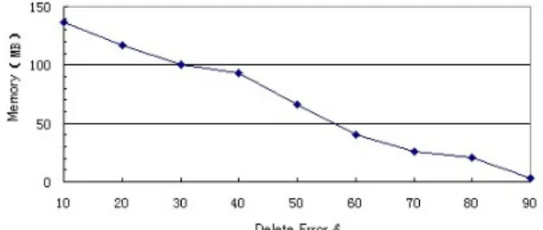
Fig.2. Memery costs using different values of errorε=δ.S
Fig.3. Computation times using different values of errorε=δ.S
It can be seen from the figures that the mining results is optimal when the value of δ is between 0.3 and 0.4. Therefore, we set the error ε =0.35S in the following experiments.
D. Therunningtimeofthealgorithm
We test the average time for processing a single transaction by FCI_Mining and compare it with algorithm A-Moment. Figure 4 shows the testing results.
Fig.4. Average time for processing one transaction It can be seen from Figure4 that algorithm FCI_Mining is faster than A-Moment. Therefore, FCI_Mining has stronger ability to detect the changes in data stream than A-Moment. The reason is that FCI_Mining detects the frequent itemsets on every gap times, instead of performing it at every time step.
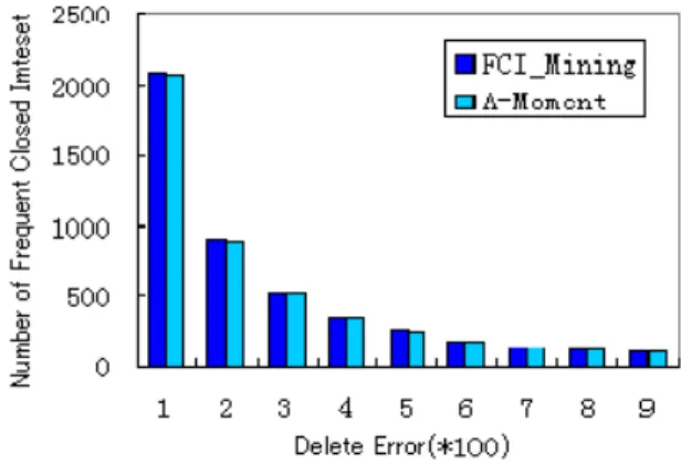
We also test the number of frequent closed itemsets detected by FCI_Mining and compare it with algorithm A-Moment. The experimental result is shown in Figure 5.
Fig. 5. Number of the frequent closed itemsets It can be seen from Figure 5 that the number of frequent closed itemsets detected by FCI_Mining is close to that of A-Moment. When the value of the minimum density is between 100 and 500, FCI_Mining detects more closed itemsets than A-Moment. The reason is that FCI_Mining deletes the infrequent itemsets on every gap times so as to retain more closed itemsets. This result suggests that FCI_Mining can obtain higher accuracy results and efficiency.
VI. CONCLUSION
We have proposed an algorithm for mining frequent closed itemsets from data streams based on a time fading module. The algorithm dynamically constructs a pattern tree, and calculates densities of the itemsets in the tree using a fading factor. The algorithm deletes real infrequent itemsets from the pattern tree so as to reduce the memory cost. A density threshold function is designed in order to identify the real infrequent itemsets which should be deleted. Using such density threshold function, deleting the infrequent itemsets will not affect the result of frequent itemset detecting. The algorithm modifies the pattern tree and detects the frequent closed itemsets in a fixed time interval so as to reduce the computation time. We also analyze the error caused by deleting the infrequent itemsets. Our experimental results indicate that our algorithm can get higher accuracy results, needs less memory and computation time than other algorithm. In our further work, we will study how to further reduce the memory cost by using the hash function in storing the frequent closed itemsets in the pattern tree. Also it is still a problem how to further reduce the computation time.
ACKNOWLEDGMENT
Firstly, I want to grant my teacher Ling Chen, without his help, I can’t finfish this work on time. Then I would like to
express my thanks to my friends, when I have puzzle, they help me try their best. And at last, I should thank my family, I can do this work so patiently under their support.
REFERENCES
[1] Y.H. Pan, J.L. Wang, and C.F. Xu, “State-of-the-art on frequent pattern mining in data streams, ” Acta Automatica Sinica, Vol.32, Issue-4, 2006, pp.594-602. [2] Y.Y. Zhu, S.S. Dennis, “StatStream: statistical monitoring
of thousands of data streams in real time [A]”, Proceedings of the 20th International Conference on Very Large Data Bases[C]. Hong Kong, China, 2002, pp. 358-369.
[3] H.F. Li, C.C. Ho and S.Y. Lee, “Incremental updates of closed frequent itemsets over continuous data streams”, Expert Systems with Applications, Vol.36, 2009, pp. 2451-2458.
[4] J. Nan and G. Le, “Research issues in data stream association rule mining”, SIGMOD Record, Vol.35, Issue-1, 2006, pp. 14-19.
[5] Y. Chi etal, “Catch the moment: Maintaining closed frequent itemsets over a data stream sliding window,” Knowledge and Information Systems, Vol.10, Issue-3, 2006, pp. 265-294.
[6] F.J. Ao etal, “An Efficient Algorithm for Mining Closed Frequent Itemsets in Data Streams,” IEEE 8th International Conference on Computer and Information Technology Workshops, 2008, pp. 37-42.
[7] J.Y. Wang etal, “TFP: An Efficient Algorithm for Mining Top-K Frequent Closed Itemsets,” IEEE TRANSACTION ON KNOWLEDGE AND DATA ENGINEERING, Vol.17, 2005, pp. 652-664.
[8] Y. Chi etal, “MOMENT: Maintaining closed frequent Itemsets over a stream sliding window [A]”, Proceedings of the 2004 IEEE International Conference on Data Mining[C], Brighton, UK: IEEE Computer Society Press, 2004, pp. 59-66.
[9] X. Liu etal, “An Algorithm to Approximately Mine Frequent Closed Itemsets from Data Streams”, ACTA ELECTRONICA SINICA, Vol.35, Issue-5, 2007, pp. 900-905.
[10] X. Ji, J. Bailey, “An Efficient Technique for Mining Approximately Frequent Substring Patterns”, Data Mining Workshops, ICDM Workshops Seventh IEEE International Conference, 2007 , pp. 325-330.
[11] S. Zhong, “Efficient stream text clustetring[J]”, Neural Networks, Vol.18, Issue-6, 2006, pp.790-798.
[12] H. F. Li, Z. J. Lu, H. Chen, “Mining Approximate Closed Frequent Itemsets over Stream,” Software Engineering, Artificial Intelligence, Networking, and Parallel/Distributed Computing, Ninth ACIS International Conference, 2008, pp. 405-410.
[13] H. Yan, Y.S. Sang, “Approximate frequent itemsets compression using dynamic clustering method,” Cybernetics and Intelligent Systems, IEEE Conference, 2008 , pp. 1061-1066.
[14] Z. N. Zou etal, “Mining Frequent Subgraph Patterns from Uncertain Graph Data,” Knowledge and Data Engineering, Vol.22, Issue-9, 2010, pp. 1203 -1218.
[15] C. Andrea, P. Rasmus, “On Finding Similar Items in a Stream of Transactions,” Data Mining Workshops (ICDMW), IEEE International Conference, 2010 , pp. 121-128.
[16] X. N. Ji, J. Bailey, “An Efficient Technique for Mining Approximately Frequent Substring Patterns,” Data Mining Workshops, Seventh IEEE International Conference, 2007, pp. 325-330.
[17] B. Bakariya and G.S. Thakur. “Effectuation of Web Log Preprocessing and Page Access Frequency using Web Usage Mining”, Vol.1 , Issue-01, 2016, pp.1-5.
Authors Profile
Caiyan Dai, Ph.D. of College of Computer Science and Technology, Nanjing University of Aeronautics and Astronautics ,China. Engaged in the research of data mining.
Ling Chen, Doctoral tutor of College of Computer Science and Technology, Nanjing University of Aeronautics and Astronautics, member of the Institute of computer IEEE. Engaged in the research of computer software, artificial intelligence, data mining, more than 100 papers published in international and domestic journals and conferences, including more than 40 papers are extracted in SCI, EI.