Towards Extraction of Spatial Relations
from Natural Language
PARISA KORDJAMSHIDI, MARTIJN VAN OTTERLO and
MARIE-FRANCINE MOENS Katholieke Universiteit Leuven
This article reports on the novel task ofspatial role labelingin natural language text. It proposes machine learning methods to extract spatial roles and their relations. This work experiments with both a step-wise approach, where spatial prepositions are found and the related trajectors and landmarks are then extracted, and a joint learning approach, where a spatial relation and its composing indicator, trajector and landmark are classified collectively. Context-dependent learning techniques, such as a skip-chain conditional random field, yield good results on the GUM evaluation data (Maptask) data and CLEF-IAPR TC-12 Image Benchmark. An extensive error analysis, including feature assessment, and a cross-domain evaluation pinpoint the main bottlenecks and avenues for future research.
Categories and Subject Descriptors: I.2.7 [Artificial Intelligence]: Natural Language Processing—Language Parsing and understanding; Text analysis; H.3.1 [Information Storage and Retrieval]: content analysis and indexing—Linguistic processing
General Terms: Experimentations, Languages
Additional Key Words and Phrases: Semantic labeling, Spatial relations, Spatial information extraction
1. INTRODUCTION
An essential function of language is to convey spatial relationships between objects and their relative/absolute location in a space. The sentence “Give me the gray book on the
large table.” expresses information about the spatial configuration of two objects (book,
table) in some space. Understanding such spatial utterances is a problem in many areas, including robotics, navigation, traffic management, and query answering systems [Tappan 2004]. Although the current work focuses on natural language processing, our long-term research considers spatial information extraction in a multimodal environment and aims to obtain and represent spatial relations using formal representations, allowing further spatial reasoning. For example, an interesting multimodal environment is the navigation domain, where we expect a robot to follow navigation instructions [Kollar et al. 2010]. When a camera is placed on the robot, it should be able to both recognize objects and their location and search for particular items based on verbal instruction. Another example is answering queries about objects’ locations using both textual descriptions and visual data; combining the evidence provided by recognizing objects in the texts and images could generate answers that are more reliable. Spatial information extraction from language could also play an important role in semantic search, i.e., extracting information based on
meaningful categories.
We recently introduced spatial role labeling problem as the extraction of generic spatial semantics from natural language [Kordjamshidi et al. 2010b]. We defined a semantic label-ing scheme to annotate spatial information. It tags natural language with the spatial roles carried by words according to the holistic spatial semantic theory (HSS) [Zlatevl 2007]. The core problem of spatial role labeling is assigning specific tags to words or phrases in natural language sentences to express their roles in terms of spatial semantics. For exam-ple, in “John is sitting on the ground”, the preposition “on” is an indicator of a spatial
relation between “John” and “the ground”. Many prepositions never carry a spatial
mean-ing, whereas some have spatial sense depending on the context. The preposition “on” in this sentence has spatial sense, though it has no such sense in the sentence “I can count on
him.” “John” is the first argument of the on-relation and is a trajector. The phrase “the ground” is the second argument of the on-relation and is a landmark. In the related
re-search in this domain, restricted languages extract very specific and application-dependent relations from text [Kelleher 2003; Tappan 2004; Li et al. 2007]. Previous research has not systematically covered spatial relation and role extraction from unrestricted natural language with machine learning methods, but this paper aims to do so. Statistical machine learning models are promising approaches to address the intrinsically ambiguous nature of spatial information in natural language.
A major obstacle when dealing with unrestricted language is the scarcity of annotated data available for training machine learning models. We therefore start with the available resources. In our leading experiments, we learn prepositions’ spatial senses by exploiting annotated data from the preposition project (TPP) employed in SemEval-2007 [Litkowski and Hargraves 2007] and then use the results of preposition disambiguation in a spatial
role labeler that identifies trajector and landmark roles. We use linguistically motivated
features and evaluate several context-dependent classification algorithms. We successfully evaluate spatial role labeling on texts from the GUM (General Upper Model spatial ontol-ogy) evaluation data [Bateman et al. 2007] and CLEF IAPR TC-12 Image Benchmark data [Grubinger et al. 2006].1
One advantage of our pipelining approach is that knowledge from another linguistic re-source is injected into the learning system. The TPP data are exploited here to solve the first part of our relation extraction algorithm, i.e., finding prepositions that have a spatial sense. We use annotated data from a larger source outside our training and test data in the extraction task, potentially increasing generalization possibilities. Errors concerning incorrectly recognizing prepositions’ spatial meaning can propagate and lead to incorrect recognition of spatial roles and relationships. Thus, the pipelined approach has difficulties competing with models that jointly learn the spatial meaning of a preposition and corre-sponding spatial roles of its arguments. Analyzing and comparing these settings provide inspiration for utilizing (other) resources for our task.
We present the first experimental study on learning to extract spatial information from unrestricted natural language. Our main contributions include the following:
—We introduce the novel spatial role labeling task, which extracts spatial relations from natural language.
1
—We present the first domain-independent English dataset with labeled data for spatial expressions, specifically designed for machine learning solutions.
—Based on linguistically oriented features, we evaluate conditional random field (CRF) algorithms and compare their suitability for the task.
—We demonstrate the injection of external data resources into the spatial role labeling task by exploiting sense-annotated prepositions from TPP and compare it to a one-step approach, limited to only using spatially annotated data.
—We provide extensive experiments to show that our approach produces good results for the spatial role labeling task.
—We extensively survey related approaches for spatial language understanding in cogni-tive science, linguistics and computer science.
—We pinpoint bottlenecks and outline future research directions.
Main structure of this article. This paper is structured as follows. In Section 2, we describe the spatial role labeling task and formally define it in Section 3.
In Section 4, we describe our approach, based on machine learning techniques, to learn the spatial role labeling task from an annotated dataset. This approach solves two main subproblems for which solutions are described subsequently. The first subproblem is iden-tifying the pivot of spatial relations, for which we learn to predict prepositions’ roles more specifically, as described in Section 4.1. The second subproblem is identifying possible
ar-guments of the spatial relations, for which we learn to predict whether parts of a sentence
can be classified as so-called trajectors or landmarks, as described in Section 4.2. Both subproblems tackle the overall goal of extracting spatial relations from text. In Section 4.3, we investigate another setting in which we classify all roles jointly, i.e., without separate classifications for spatial indicators and trajectors/landmarks. Section 4.4 reports which algorithms, based on probabilistic graphical models, are employed by both subproblems.
In Section 5, we present and discuss a series of experiments. After introducing the main structure and rationale of the experiments, we show results for several datasets and perform an additional feature analysis. We give results in quantitative form but also present a quali-tative analysis to show the effectiveness of the approachs. To complement the error analysis and see how well the learned classifiers generalize new data, we evaluate them on several texts from different subject domains than the training domain. After the experiments, in Section 6, we discuss related lines of research on spatial information representation and extraction in cognitive science, linguistics and machine learning. Section 7 concludes this article and outlines prominent research directions in spatial language processing.
2. THE SPATIAL ROLE LABELING TASK
As discussed above, spatial information plays an important role in many applications [Gal-ton 2009]. However, its automatic recognition in natural language expressions is unde-veloped or, when addressed, limited to recognizing coarse-grained and brittle information added to predicates and mainly expressed by verbs.
To highlight some general aspects of spatial semantics, consider the following two sen-tences (taken from [Bateman et al. 2010]):
(1) He left the institute an hour ago. (2) He left the institute a year ago.
building, and the sentence is about physically leaving the building and going somewhere else. This change directly amounts to a physical and spatial relocation. The second sen-tence expresses a more fundamental change: the person has apparently quit his job at the institute. The second type of spatial change is more involved and less material. Another set of examples is as follows:
(3) The computer is on the table and the mouse is to the left of it.
(4) The party leader could be considered at the far left of the political spectrum. The first sentence expresses two explicit physical relations about objects on a table. The second sentence uses a similar relation ”at the far left of”, but its meaning is more concep-tual. Only drawing this ”political spectrum” on a piece of paper allows one to put the party leader on its left side.
These examples illustrate some of the challenges in spatial language understanding. Similar lexical items can provide different spatial meanings. Conversely, two different descriptions may have a similar semantic interpretation:
(5) Looking over his right shoulder, he saw his dog sitting quietly. (6) The dog sat quietly on the floor to his right.
In the sentences (1) and (2), the spatial information is mainly expressed through a verb, whereas the other examples primarily use prepositions. Furthermore, some information is not explicitly represented in the words but can be inferred from common sense. For example, one can infer that the mouse is on the table in sentence (3). This sentence also includes a related inference step resolvable at the linguistic level. An anaphora resolution step attaches it to the computer before determining the spatial semantics. It could refer to
the table, in which case the spatial semantics also differ.
Despite the variations in spatial information in natural language expressions, a sen-tence can essentially express spatial relations between objects. For example, the third sentence contains an on-relation between the computer and the table. Another relation is that the mouse is to the left of the computer. Such relations, denoted on(computer,table) and toTheLeftOf(mouse,computer), form the starting point of any system that processes spatial information in natural language. In on(computer,table), we can distinguish the dif-ferent spatial roles of phrases in a sentence: on expresses a predicate (or, relation) and
computer and table are arguments with their own roles. Our main concern in this article is extracting such spatial relations.
We define spatial role labeling as the automatic labeling of words or phrases in
sen-tences with a set of spatial roles. The roles take part in one or more spatial relations
expressed by the sentence. The sentence-level spatial analysis of texts characterizes spatial descriptions, such as determining the objects’ spatial properties and locations to answer
”what/who” and ”where” questions. The spatial indicator (typically a preposition)
es-tablishes the type of spatial relation, and other constituents express the participants of the spatial relation (e.g., entities’ locations). The following sentence is an example:
Give me the[gray book]tr[on]si[the big table]lm.
Our spatial role set consists of trajector (tr), landmark (lm) and spatial indicator (si) (and
none otherwise) [Kelleher 2003; Zlatevl 2007; Kordjamshidi et al. 2010b]. The above
sentence contains several subsequences labeled with these roles. They are as follows: —Trajector: the entity whose (trans)location is of relevance. The book is the main entity
of which location is specified in the sentence. The trajector can be static or dynamic, a person or an object, or even a whole event. Alternative terms used in the literature are
local/figure object, locatum, referent or target.
—Landmark: the reference entity in relation to which the location or trajectory of the trajector’s motion is specified. The main entity’s location designator (the trajector, the
book) is the table. Other terms for landmarks are reference object, ground, or relatum.
—Spatial indicator: the tokens that define constraints on the spatial properties, such as the trajector’s location with respect to the landmark (e.g., in, on). A spatial indicator expresses a relation (or predicate) with the landmark and trajector as its arguments. Spatial indicators explain the types of spatial relations and are often prepositions but can also be verbs and nouns among other parts of speech. These indicators are the pivot of spatial relations.
Other conceptual aspects, such as motion indicators, indicate specific spatial motion in-formation (usually specified in terms of verbs); frame of reference and the path of a motion are influencing concepts for spatial semantics and roles [Zlatevl 2007]. However, we restrict our focus to prepositions conveying spatial information.
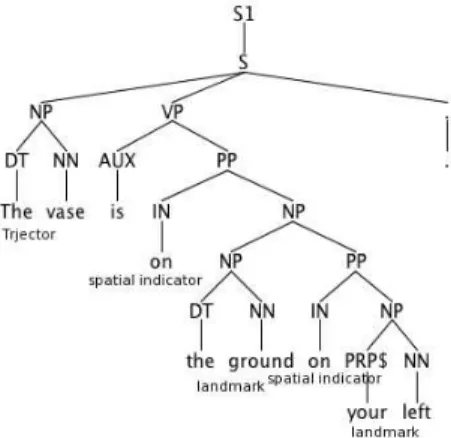
Fig. 1. Parse tree labeled with spatial roles. Spatial role labeling is a special type
of semantic role labeling, and, as with semantic roles, the spatial relations sup-ported by the roles contribute to a sentence’s semantic frame recognition [M`arquez et al. 2008]. In semantic frame labeling, a predicate is identified and dis-ambiguated, and its role arguments are recognized. In spatial role labeling, the spatial indicator is identified (instead of the verb predicate) and disambiguated, and its semantic role arguments including the trajector and landmark, are found.
However, differences between these two tasks exist. In spatial role labeling, the roles are more specific regarding their semantics; there is no direct correspon-dence between the sentence’s semantic
structure based on traditional semantic frames (patient, agent) and the spatial semantics’ structure. In the above example, FrameNet’s “Giving” frame provides the semantic type
Locative relation; the Place where the Donor gives the Theme to the Recipient. The
lo-cation refers to the place where the give is performed, and not the lolo-cation of the book, mentioned in the prepositional phrases. Moreover, both the formal and informal (prag-matic) spatial expression meanings in natural language are highly dependent on lexical details, the ontological structure of spatial information spaces, and the embedding of ex-tracted information into existing spatial knowledge.
Another difference between spatial role labeling and semantic role labeling is that no large annotated corpora were available from which spatial roles could be learned directly. New data resources were needed to apply machine learning techniques. In this respect, breaking the problem into parts and utilizing existing linguistic resources have the
advan-tage of limiting the training examples that must be labeled. These external resources could improve the performance of the spatial role labeling task, which is evaluated in this paper. General spatial relation extraction presents many challenges concerning task-specific ambiguities and difficulties. However, there is not always a direct mapping between a sentence’s grammatical structure and its spatial semantic structure. This issue is more challenging in complex spatial expressions that convey several spatial relations. The sim-ple examsim-ple below shows that grammatical dependencies cannot always identify spatial dependencies and connections:
The vase is on the ground on your left.
The dependency tree relates the first appearance of “on” to the words “vase” and “ground”. This process produces a valid spatial relation connecting the right trajector to the right land-marks. If we systematically follow the grammatical clues and information, then the second appearance of “on” connects the “ground” and “your left”, producing a less meaningful spatial relation in terms of trajector, landmark and spatial indicator (“ground on your left”), Figure 1 shows the related parse tree. When confronted with more complex relations and nested noun phrases, deriving “spatially valid” relations is not straightforward and highly dependent on the lexical meaning of words. However, recognizing the right prepositional phrase (PP) attachment during syntactic parsing can improve the identification of spatial arguments.
Other linguistic phenomena, such as spatial-focus-shift and ellipsis of trajector and
landmark [Li et al. 2007], make extraction more difficult. Spatial motion detection and recognition of the frame of reference are additional challenges that are not treated here.
3. PROBLEM DEFINITION
The spatial role labeling task finds spatial relations in natural language sentences, each of which includes a spatial indicator and its arguments. We assume that the sentence is a priori partitioned into a number of segments. The segments could be words, phrases or arbitrary subsequences of the sentence. More formally, letS be a sentence defined as a sequence ofNsegments:
S=w1, w2, . . . , wN
We define a set of roles: roles = {trajector,landmark,spatial indicator,none}, and each segment in the sentence can be assigned one or more of these roles. Each spatial relation in sentenceSis a triple
wspatial indicator, wtrajector, wlandmark
wherewspatial indicator,wtrajectorandwlandmarkare three distinct segments ofS, denoting the parts ofSthat represent the spatial indicator and its trajector and landmark arguments, respectively. For any spatial relation, the value of the trajector (or landmark) can be “unde-fined”, meaning that no segment inSrepresents the trajector (or landmark). In those cases, we call the trajector (or landmark) implicit, as in the sentence “Come over here”, where the trajector “you” is only implicitly present.
the indicator functionIdefined over all segmentswofS:
I(w) =
(
1, ifwis a spatial indicator
0, otherwise
We assume that spatial indicators overlap with neither each other nor trajectors and land-marks. In other words, for any sentence S, if w andw′ are two segments of
S, then
I(w) = 1andI(w′) = 1imply that
w∩w′ =∅. Because trajectors and landmarks are spatial indicator arguments, we define two indicator functions relative to a given spatial in-dicatorsin sentenceS. The set of trajectors (landmarks) with respect to spatial indicator
sis denotedTs(Ls), induced by indicator functionsTsandLsdefined over all segments
inS. For a spatial indicators, its trajector and landmark cannot overlap with each other or
sitself (though they can be undefined, as mentioned earlier).
Although we have defined spatial indicators, trajectors and landmarks as arbitrary seg-ments of a sentence, we focus on single words, each as one segment. However, a phrase in the sentence commonly plays a role, and we thus assume that the head word of the phrase is the role-holder. A head word determines its phrase’s syntactic type; analogously, it is a stem that determines the semantic category of its component’s compound. The other elements of a phrase modify the head. For example, in ”the huge blue book”, ”book” is the head word, and ”huge” and ”blue” are modifiers. In our data, the labeling scheme reflects this fact and only assigns roles to head words and labels the remaining words (e.g., modifiers) as “none”. Hence, a sentence is hereafter assumed to be a sequence of words.
Our ground-truth data include sequences, each of which contains exactly one (labeled) spatial indicator with all possible trajectors and landmarks. A sentence can thus provide multiple examples, up to the number of its contained spatial indicators. We formally define each sentence in the corpus as a sequence of wordshw1, . . . , wni. Letkbe the number
of prepositions in a sentences; sthen induceskexamplese1. . . ek, where examplesei
and ej have the same spatial indicator for no i and j. Each ei (i = 1. . . k) is a
se-quenceh(w1, l1), . . . ,(wn, ln) in which each wordwi (i = 1. . . n) is tagged such that
i) at most, onewjgets a labellj= spatial indicator; ii) some words get a labeltrajector
orlandmark, if they are a trajector or landmark of the spatial indicatorwj; and iii) the
remaining words get a labelnone. If a preposition is not spatial, all words in the example are tagged withnone. As an illustration, consider the following sentence, which gives two examples:
A girl and a boy are sitting at
none trajector none none trajector none none sp.indicator
none none none none none none none none
the desk in the classroom.
none landmark none none none none trajector sp.indicator none landmark
The sentence is labeled twice, each time with a different indicator. Using our indicator functions, we have
I={at,in} Tat={girl,boy} and Lat={desk}
The spatial relations for this sentence are the triples produced by the following (we only account for head words in the role-playing phrases):
{at} × {girl,boy} × {desk}=hat,girl,deski,hat,boy,deski {in} × {desk} × {classroom}=hin,desk,classroomi
An example with an implicit trajector is the following sentence:
Go under the bridge
none spatial indicator none landmark In this case, we derive the spatial relation using
I={under} and Tunder=∅ and Lunder={bridge}
which results inhunder,undefined,bridgeias the corresponding spatial relation.
This article takes a given corpus of sentences tagged with spatial indicators, trajectors and landmarks, giving a multitude of sequence examples, and constructs (i.e., learns) an automated spatial relation extraction method that can be employed successfully on unseen data.
4. APPROACH
The problem definition leads to a similar problem as semantic role labeling (SRL), where words are classified based on a known predicate (a verb). In spatial role labeling, the spatial indicator is the pivot (i.e., predicate) of the spatial relation. A spatial indicator can be from various lexical word classes, although the most dominant form is the preposition. In SRL, one can start from a verb and find roles related to it, but in spatial role labeling, one must first find the sense of the pivot (i.e., the preposition). Sometimes, a proposition has a spatial sense, but that same preposition might not have a spatial sense in a different context.
In our approach, the set of roles is{trajector,landmark,spatial indicator,none}, and we use an additional term undefinedto highlight the existence of implicit trajectors or landmarks;undefineddoes not appear in the annotated data, nor is it learned or predicted by our classifiers. It solely serves as a place-holder for missing elements if the three com-ponents of a spatial relation cannot be explicitly found in a sentence (Algorithm 1 provides further explanation). The set of all spatial relations in a sentenceS, denotedSR, is defined thus (wheres, t, lare head words inS):
SR =hw, w′
, w′′
i |w∈I, w′
∈Tw, w′′∈Lw
In this definition, three functions should be estimated. First, the functionIis needed; it takes a word in the sentence as an input and estimates whether it is a spatial indicator. We employ a general probabilistic classifier; for spatial indicators, we learn a functionIˆ
representing the probability that a word is spatial, given some features about sentenceS. To get the (deterministic) indicator functionI, we compute (usingr={spatial,nonspatial})
I(w) =
(
1, if spatial = arg maxx∈rIˆ(x|w, f(w, S))
optimized over training data, wheref(w, S)denotes a set of features derived from sentence
Sand wordw.
Indicating which words in the sentence have the trajector or landmark role requires two other functions, given that we know that some word sis a spatial indicator. Because
the parameters for both trajectors and landmarks are the same (i.e., the spatial indicator), we can combine them into a multi-class classification problem that classifies words in a sentence (i.e., head words) intor′ ={trajector
,landmark,none}. We call this function
ˆ
R, and it takes a spatial indicator and tags words with these roles. We use a probabilistic classifier here, and to obtain deterministic classifications for landmarks and trajectors, we first compute
rw,s= arg max
x∈r′ ˆ
R(x|w, s, f(w, s, S)) (2) wherewis a word in sentenceS,sis a spatial indicator,f(w, s, S)denotes a set of fea-tures defined over the wordw, the spatial indicators, and the sentenceS. This process maximizes a probability function given a set of features. The details of this function are described in the next section. We continue with
Ls(w) = ( 1, ifrw,s= landmark 0, otherwise Ts(w) = ( 1, ifrw,s= trajector 0, otherwise
From Equations 1 and 2, we see that a natural pipelined task decomposition presents itself. We can first find words that potentially carry a spatial sense (I(s) = 1), and we then find the corresponding trajectors and landmarks for each pivot.
The general structure of our pipeline approach consists of the following steps, outlined in subsequent sections:
—Finding spatial indicators: The first task consists of labeling parts of an input sentence
S that play the spatial pivot role or finding the preposition with spatial sense. Sec-tion 4.1 describes this step, which utilizes TPP data to learn the labeling task. As we see below, we reduce this step to finding potential spatial indicators by only considering a sentence’s prepositions.
—Finding spatial arguments: The second task consists of classifying parts of an input sentenceSthat play the landmark or trajector roles, given a (spatial) pivot. We employ two annotated datasets (CLEF and GUM (Maptask)) and describe it in Section 4.2. In an additional relation extraction phase, we assemble the results of the previous two steps to form spatial relation triplets with spatial indicators and their trajector and landmark arguments (see also Algorithm 1). This step is straightforward and involves no learning. We also investigate an alternative approach in which we tackle both steps jointly:
—Finding spatial indicators and their arguments jointly: In this task, we do not use a separate preposition disambiguation step but instead learn to tag all words in a sentence jointly. The examples in the dataset are used to train a single classifier that assigns the spatial indicator, trajector, and landmark roles simultaneously. Classifications can there-fore correlate without using additional data resources (e.g., TPP). Section 4.3 describes this approach.
The remainder of this section describes the features and algorithms we designed and im-plemented for the spatial relation recognition task.
4.1 Learning Spatial Indicators
Various lexical categories (e.g., verbs, adjectives) can express spatial information, but prepositions primarily do so [Baldwin et al. 2009]. However, because prepositions of-ten have different senses [Tratz and Hovy 2009; Litkowski and Hargraves 2007], we wish to recognize whether they convey a spatial sense. The sense of prepositions can be dis-ambiguated by machine learning methods, as a large corpus exists for it. We consider prepositions because of their importance and the feasibility of the disambiguation task.
According to the aforementioned formalization, the setIcontains only prepositions and
I(w) = 1 holds only for prepositions with spatial sense. We aim to promote the use
of a specific training scheme for preposition sense disambiguation and not perform other linguistic techniques to recognize them. The locatives recognized by SRL might be a solution, but this is often not true. The following two examples stem from the preposition disambiguation dataset (TPP) [Litkowski and Hargraves 2007].
(i) He saw Owen redden with pleasure and
laughed flinging an arm about his shoulders . . .
(ii) This project compares assumptions incorporated into
social policies about these obligations . . .
Prep POS DepRel SRL sense
about(i) IN NMOD Arg1 spatial
about(ii) IN NMOD Arg1 topic
Table I. Assigned labels by a POS tagger, dependency tree and SRL to ”about” with two senses.
Table I shows the labels assigned by a part-of-speech (POS) tagger, a dependency parser, and SRL to the preposition ”about”. The parse tree, the dependency tree and even the semantic role labeler could not distinguish between two senses of the preposition ”about”. We therefore propose to learn these senses from a corpus labeled with senses (TPP) pro-vided for the preposition disambiguation task (SemEval07) [Litkowski and Hargraves 2007], featuring the categorySpatialSenseamong others.
More specifically, the componentIˆperforms this preposition disambiguation task in Equation 1. It uses the following linguistically motivated features and the preposition contextual features that we aim to classify:
—The preposition itself
—By exploiting the dependency parser:
—The words directly dependent on the preposition (head1)
—The words on which the preposition is directly dependent (head2) —For the predicates which have a dependency relation with the preposition:
—All words that are arguments of the predicate other than the preposition are added using a semantic role labeler
For all extracted words satisfying the above conditions, the following features are also included:
—The part-of-speech tag (POS)
—The type of dependency relation (DPRL)
—The semantic role labels and, for predicates, the sense of the predicate (if assigned) We present a sentence containing a preposition and the extracted features as an example.
He saw Owen redden with pleasure, and laughed , flinging an arm about his shoulders ... {P reposition(′′ about”), P reposition P OS(′′ IN”), P reposition DP RL(′′ N M OD”), P reposition isarg(′′ A1 arm.01”), head1(′′
arm”), head1Lemma(′′
arm”), head1 P OS(′′
N N”), head1 DP RL(′′
OBJ”), head1 sense(′′
arm.01”), head1 isarg(′′
A1 f linging.01”), head2(′′shoulders”), head2 lemma(′′shoulder”),
head2 P OS(′′N N S”), head2 DP RL(′′P M OD”),
head2 isarg(shoulders.01), head2 sense(”shoulders.01”)}
To identify the spatial prepositions, we use the TPP data provided for the preposition dis-ambiguation task, SemEval07 [Litkowski and Hargraves 2007]. We extract the features from the training and test data and use a maximum entropy and a Naive Bayes classifier to disambiguate the prepositions’ sense. This process results in a binary classification of a preposition’s spatial or nonspatial sense.
4.2 Trajector and Landmark Classification
As explained in Section 4, a multi-class classifierRˆmust be trained to map each wordw
onto a class label from the set{trajector,landmark,none}, given a spatial indicators. Because spatial indicator features are used to classify the roles of words in the sentence, the spatial indicator must be known before classifying trajectors and landmarks. Hence, we utilize the first step of preposition sense disambiguation, described in the previous section, to recognize the spatial indicators first, after which its arguments (trajectors and landmarks) can be classified. The generic feature set used in Equation 2 can now be defined in more detail using three different sorts. The first set of features relates to the word that we aim to classify (f1(w)), the second includes the features of the spatial indicator of which the word may be an argument (f2(s)), and the third contains the features that relate the word to the sentence’s indicator (f3(w, s)). SRL inspired these features, but they center on the spatial indicator. As mentioned, features are defined for head words.
—Features of a wordw—f1(w): —The word (form) ofw. —The part-of-speech tag.
—The dependency to the syntactic head in the dependency tree. —The semantic role.
—The subcategorization of the word (sister-nodes of its parent node in the tree). —Features of the spatial indicators—f2(s):
—The spatial indicator word (form). —The subcategorization ofs.
—Relational features ofww.r.t.s—f3(w, s): —The path in the parse tree from thewto thes.
—The number of nodes on the path betweensandwnormalized by dividing over the number of all nodes in the parse tree (to obtain an integer value it is reversed and rounded afterwards):
distance =#Nodes on the path betweensandw
#Nodes in the parse tree
Take the following sentence as an example.
”The vase is on the ground on your left.”
Here, the input features for classification of ”vase” w.r.t. the first ”on” are: ”vase”,”NN”,”SBJ”,”A0”,NP-VP | {z } ”on”,”NP” | {z } NN↑NP↑S↓VP↓PP↓IN,”true”,”3” | {z } f1(w) f2(w) f3(w, s)
A semantic role labeler is typically trained on a large external dataset. Using assigned semantic roles as features brings in additional knowledge, which may not be present in the dataset used to train the spatial role labeler. This issue encourages the use of the semantic roles as features.
The task is now a multi-class classification problem in which each word, represented by a feature vector, is separately classified, assuming that these classifications are independent. We use such a model in our initial experiments. In subsequent models, words are also described by their features, but the class to which they are assigned depends not only on their own values but also on the other feature vector values and relations among the various classes. The obtained class of a word may constrain the class of the next word.
We therefore employ several conditional random field (CRF) models. In these models, a sentence is a sequence of observations (i.e., words),hw1, . . . , wNi, which can be
repre-sented using a probabilistic graphical model. Each observation can be described in terms of the described feature vectors, and the model outputs a label for each word in the sequence. After recognizing the trajector and landmark given a spatial indicator, we have all the re-lation elements. Rere-lation extraction is performed in a straightforward way, by assembling all extracted spatial indicators, trajectors, and landmarks and combining them into spatial relation triplets. Algorithm 1 shows the entire process, based on preposition disambigua-tion and trajector/landmark classificadisambigua-tion.
4.3 Learning Spatial Relations without a Priori Spatial Indicator Classification The spatial role labeling task can be seen as a joint classification task: to predict each triplet of segments as being in the indicator-trajector-landmark relation or not. In the previous section, we outlined a pipelining method for spatial role labeling, where a preposition (i.e., spatial indicator) is classified as spatial or nonspatial and the trajector and landmark are then sought for the obtained spatial indicators. Our focus on prepositions added one constraint to this task; the indicator should be a preposition (a realistic bias in English). The main purpose of this pipeline approach is to exploit a large external data source (TPP) for spatial sense disambiguation.
Combining two steps of the pipeline provides another option for learning spatial rela-tions. We could omit the first step of using a dedicated classifier for spatial sense recog-nition, and learn to assign all spatial roles jointly, i.e., tagging words with trajector,
Algorithm 1 Spatial-Relation-Extraction( S : sentence ) returns relationsSR
1: {preposition disambiguation} 2: for all w∈Sdo
3: EstimateIˆ(w)by training a probabilistic classifier and
4: construct the setIof all spatial indicators of the sentenceS.
5: for all s∈I do
6: {trajector and landmark classification} 7: for allw∈Sdo
8: Estimate a probabilistic multi-class classifierRˆand
9: construct the setsTsandLsaccording to the assigned labels. 10: ifTs=∅thenTs← {undef ined}
11: ifLs=∅thenLs← {undef ined} 12: {relation extraction}
13: SR←SRShs, t, li |t∈Ts, l∈Ls 14: returnSR
landmark, spatial indicatorornone, based on a training dataset. To train the
classi-fier, we can employ a procedure and examples as in the pipeline setting, but the classifier must then learn one more label (spatial indicator). To test and evaluate the classifier on a new (unlabeled) sentenceS, we see thatS can contain several prepositions with spatial sense and many trajectors and landmarks, whereas the classifier can only assign a single label to each word. The solution we use here is to, again, generate multiple examples fromS, where each example contains a designated pivot with specific features extracted for that word (e.g., path features from words to the pivot). For each example, the words are classified using these features. One must theoretically generate as many examples as there are words inS; in our practice, it suffices to do this procedure only for pivots that are prepositions. The main advantage of this setting is that the learning algorithm gets the freedom to classify trajectors, landmarks and indicators in the context of one another.
In the relation extraction step, we perform the same general steps as in Algorithm 1, dif-fering primarily in that we take all prepositions as possible spatial indicators in the preposi-tion disambiguapreposi-tion phase (lines1–4) and that the classifierRˆnow uses all roles, including
spatial indicator. This fact allows multiple words to be classified as spatial indicators in
one sequence and could in principle allow the extraction of spurious relations. However, due to the learning bias (i.e., each example contains only one targeted preposition), we discovered that spurious relations are rarely extracted. While on the one hand, the joint setting enables a learning algorithm to use the information in the data without depending on external data resources, on the other hand, there is a hazard of becoming specialized to the spatial preposition distribution in the available data. The experimental results section empirically investigates this trade-off.
4.4 Algorithms
A conditional random field (CRF) is a state-of-the art model for context-dependent classi-fication. A CRF is an undirected graphical model or Markov random field, conditioned on a set of observationsX to predict a set of output variablesY. We defineG= (V, E)as an undirected graph (with verticesV and edgesE) such that a nodev∈V corresponds to each random variable andV =X∪Y. We denote an assignment toX byx, an
assign-ment to a setA⊂XbyxA, and similarly forY. If each random variabley∈Y obeys the
Markov property with respect to G, then(Y, X)is a conditional random field. This model represents a probability distribution over a large number of random variables by a product of local functions that each depend on a small subset of variables. This factorization of the global probability distribution makes learning and inference feasible.
A CRF generally defines a probability distributionp(y|x)as follows:
p(y|x) = 1
Z(x)
Y
AΨA(xA, yA)
in whichΨA(xA, yA)is a potential function, whereΨA : Vn → ℜ+ andZ(x)is the
normalization factor: Z=X y Y AΨA(xA, yA) and ΨA(xA, yA) = exp K(A) X k=1 λAkfAk(xA, yA)
Finally the conditional probability is the following:
p(y|x) = 1 Z(x) Y ΨA∈G exp K(A) X k=1 λAkfAk(xA, yA)
For the CRF experiments we use Mallet2and GRMM:3
—Linear-chain CRF. The structure of graphGis theoretically arbitrary; however, when modeling sequences (in our case, words of a sentence), the simplest graph is a linear-chain CRF in the form of a (often first-order) Markov linear-chain [Lafferty et al. 2001; Sutton and MacCallum 2006]. In this setting, the spatial role label of a word in the sentence de-pends on the label of word in the previous position. Considering sequential relationships can increase the learning model’s accuracy. The conditional probabilityp(x|y)is
1
Z(x)
YN
t=1Ψt(yt−1, yt, x)
whereX = (x1, . . . ,xK)is a sequence or other structural set of observations andY = (y1, . . . ,yK)is the corresponding set of labels assigned toX. In the spatial role labeling
task,X ranges over the words of a sentence, whileY ranges over the classes trajector (tr), landmark (lm), spatial indicator (siin the joint setting) or none of these (none).
Ψt(yt−1, yt, x)is a potential function, which is a real-valued function that captures the
degree to which the assignmentytto the output variable fits the transition fromyt−1and
X. The potentials typically factorize according to a set of featuresF ={fk}such that Ψ(yt−1, yt, x) = exp{PKk=1λfk(yt−1, yt, x)}.
The linear chain CRF setting of Mallet uses a forward-backward algorithm to compute the marginal distributions and the Viterbi algorithm to compute the most probable se-quence label assignment. For our task, allowing transitions unobserved in the training
2
http://mallet.cs.umass.edu/download.php 3
y2 y1 X1 y3 y4 X5 X4 y6 y5 X6 X2
The book is on the table . X3
y7
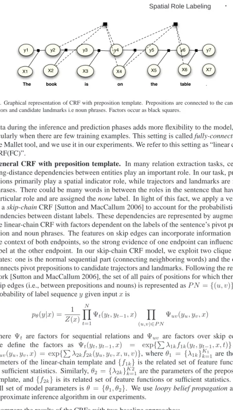
X7
Fig. 2. Graphical representation of CRF with preposition template. Prepositions are connected to the candidate trajectors and candidate landmarks i.e noun phrases. Factors occur as black squares.
data during the inference and prediction phases adds more flexibility to the model, par-ticularly when there are few training examples. This setting is called fully-connected in the Mallet tool, and we use it in our experiments. We refer to this setting as “linear chain CRF(FC)”.
—General CRF with preposition template. In many relation extraction tasks, certain long-distance dependencies between entities play an important role. In our task, prepo-sitions primarily play a spatial indicator role, while trajectors and landmarks are noun phrases. There could be many words in between the roles in the sentence that have no particular role and are assigned the none label. In light of this fact, we apply a version of a skip-chain CRF [Sutton and MacCallum 2006] to account for the probabilistic de-pendencies between distant labels. These dede-pendencies are represented by augmenting the linear-chain CRF with factors dependent on the labels of the sentence’s pivot prepo-sition and noun phrases. The features on skip edges can incorporate information from the context of both endpoints, so the strong evidence of one endpoint can influence the label at the other endpoint. In our skip-chain CRF model, we exploit two clique tem-plates: one is the normal sequential part (connecting neighboring words) and the other connects pivot prepositions to candidate trajectors and landmarks. Following the related work [Sutton and MacCallum 2006], the set of all pairs of positions for which there are skip edges (i.e., between prepositions and nouns) is represented asP N ={(u, v)}; the probability of label sequenceygiven inputxis
pθ(y|x) = 1 Z(x) N Y t=1 Ψt(yt, yt−1, x) Y (u,v)∈P N Ψuv(yu, yv, x)
where Ψt are factors for sequential relations and Ψuv are factors over skip edges.
We define the factors as Ψt(yt, yt−1, x) = exp{Pλ1kf1k(yt, yt−1, x, t)} and
Ψuv(yu, yv, x) = exp{Pλ2kf2k(yu, yv, x, u, v)}, whereθ1 = {λ1k}Kk=11 are the
pa-rameters of the linear-chain template and{f1k}is the related set of feature functions
or sufficient statistics. Similarly,θ2 ={λ2k}Kk=12 are the parameters of the preposition template, and{f2k} is its related set of feature functions or sufficient statistics. The
full set of model parameters isθ = {θ1, θ2}. We use loopy belief propagation as the approximate inference algorithm in our experiments.
We compare the results of the CRFs with two baseline approaches:
sentence independently using a standard maximum entropy classifier.
—Simple baseline. To encourage the use of machine learning, a simple baseline is em-ployed: given a spatial preposition, the first head word before the preposition is taken as the trajector and the head word after the preposition as the landmark. There is no learn-ing from data in this settlearn-ing, but the dependency tree is exploited to discover dependent headwords.
5. EXPERIMENTAL STUDY
In this section, we report on a series of experiments to evaluate various components of the spatial role labeling and relation extraction tasks.
5.1 Structure and Goals of the Experimental Setup
We present our leading research questions and identify the sections where we experimen-tally answer those questions.
—Which data resources are available, or can be generated, to learn the spatial role
label-ing task from data?
We answer this question in Section 5.2. In our experiments, we clearly want to solve the spatial role labeling task for unrestricted natural language input. However, we are limited by the amount of available data for machine learning. We describe our novel data resources and summarize their statistics.
—How can we detect the spatial sense of prepositions using available resources?
We answer this question in Section 5.3. We first investigate whether other resources (e.g., locatives obtained from SRL) can help and what benefits lie in directly learning the spatial sense from a large external and available data source (TPP).
—If we assume that the spatial sense of a preposition is known or learned beforehand, how
can we learn its corresponding trajectors and landmarks from data?
In Section 5.4, we present various classifiers that take a given (spatial) preposition as input, and label the corresponding arguments (landmark and trajector) of the predicate the preposition represents.
—What benefits lie in the sequential nature of finding the spatial sense of a preposition
and then finding trajectors and landmarks (the so-called pipeline technique)?
In Section 5.4.1, we first decouple the two problems and focus solely on the situation in which the spatial sense is known perfectly. In Section 5.4.2, we investigate two different situations where we fully automate the task, i.e., we use the preposition disambiguation output as input for spatial relation recognition. Without ground-truth data on the spatial sense of the prepositions, some landmarks or trajectors cannot be found because this spatial sense is classified incorrectly. We investigate a setting in which unknown prepo-sitions are classified as spatial by default and another in which they are nonspatial by default.
—What benefits lie in jointly recognizing spatial indicators, trajectors and landmarks, and
how can long-distance dependencies help in this setting?
In Section 5.4.3, we investigate an approach in which we learn to tag words with an extended label set that includes spatial indicators. This process side-steps preposition disambiguation as a separate phase; thus, classifications depend only on the information in one training dataset.
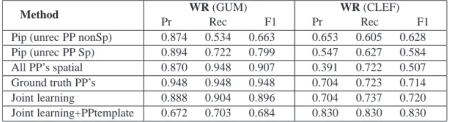
—How do different pipelining methods affect the accuracy of the whole-relation
extrac-tion?
In Section 5.5, we perform experiments in which we measure the accuracy of different pipelining techniques on the whole-relation extraction (thus finding the correct spatial indicators, i.e., prepositions and their correct landmarks and trajectors).
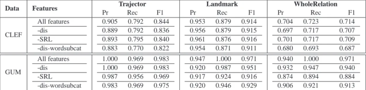
—What is the effect of the used features on the extraction task? Section 5.6 discusses the effects of leave-one-out feature analysis.
—What is the cross-domain performance of the approach on an unrestricted natural
lan-guage text that contains both spatial and nonspatial information?
In Section 5.7, we apply our system to several small, general, and unrestricted natural language texts to evaluate performance on data outside the training domain.
—What are the main sources of errors in our approach?
In Section 5.8, we investigate the errors made in50sentences of our dataset. We can distinguish five general categories of errors, including nested spatial relations and spa-tial focus shift. The errors caused by different model characteristics and different data domain characteristics are investigated in two separate subsections.
5.2 Dataset Description
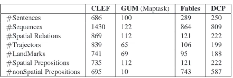
For our experimental analysis, we use several manually annotated datasets. We describe their characteristics and usefulness for our study in this section. Statistics for the corpora are presented in Table II.
—TPP dataset For the preposition disambiguation task, we employ the standard test and training data provided by the SemEval-2007 challenge [Litkowski and Hargraves 2007]. It contains 34 separate XML files, one for each preposition, totaling over 25,000 in-stances with 16,557 training and 8,096 test example sentences; each sentence contains one example of the respective preposition.
—GUM (Maptask) dataset Because the spatial role labeling task is newly defined, there is no annotated English corpus available. However, the GUM (General Upper Model) evaluation data [Bateman et al. 2007], comprising a subset of a well-known corpus for spatial language is a useful dataset. It has been used to validate the expressivity of spatial relations in the GUM ontology. Currently, the dataset contains more than 300 English examples and 300 German examples. We used 100 English samples in this corpus that are originally from the Maptask corpus. The GUM-annotation for this sentence is an example:
”The destination is beneath the start.”
is:
SpatialLocating (locatum ”destination”, process ”being”, placement GL1 (relatum ”start”, hasSpatialModality UnderProjectionExternal)).
Here, relatum and locatum are alternative terms for landmark and trajector. Spatial
modality is the spatial relation mentioned in the specific spatial ontology. The corpus
contains 65 trajectors and 69 landmarks appearing in 112 spatial relations. Each sen-tence produces spatially labeled sequences in the number of its prepositions: 122 se-quences for GUM (Maptask). Although complete phrases are annotated in this dataset, we only use a phrase’s headword with trajector (tr) and landmark (lm) labels and their
spatial indicator (si). Using this small corpus to evaluate our approach for a very domain-specific corpus, including only instructions and guidance for finding the way on a map, is beneficial.
CLEF GUM (Maptask) Fables DCP
#Sentences 686 100 289 250 #Sequences 1430 122 864 809 #Spatial Relations 869 112 121 222 #Trajectors 839 65 106 199 #LandMarks 741 69 95 188 #Spatial Prepositions 735 112 121 222 #nonSpatial Prepositions 695 10 743 587
Table II. Data statistics.
—CLEF dataset Because the available dataset is small, an additional dataset4was
anno-tated, based on textual descriptions of 400 images of the IAPR TC-12 Image dataset [Grub-inger et al. 2006], hereafter the CLEF dataset. This dataset generated an additional 686 English sentences with 869 spatial relations. The CLEF dataset contains images taken by tourists with descriptions in several languages. The text describes objects with their absolute and relative positions in the image. It is therefore a rich resource for spatial information. However, the descriptions are not always limited to spatial descriptions and are thus less domain-specific and contain free image explanations.
We have annotated the textual descriptions with spatial roles of trajector (tr), landmark (lm) and their corresponding spatial indicator (si). Roles are assigned to the headwords of the phrases only. Two annotators provided annotations (325 sentences) and we investigated the inter-annotator agreement [Carletta 1996]. The Kappa value is 0.896 with a 95% confidence interval (0.882–0.910).
As mentioned above, we only consider prepositions as spatial indicators. This restriction is natural in English texts and especially for our data. Ignoring lexical categories other than prepositions has a trivial influence on our experiments with this corpus. Three exceptional cases exist in CLEF, where the words crossing, supporting and away are tagged as spatial indicators and this is the case for seven sentences in GUM (maptask) dataset. Furthermore, in compound verbs such as ”surrounded by”, the preposition, here ”by”, is annotated as the indicator although it is attached to the verb. However, for mapping to the spatial relation semantics, having the correct pp-attachment is an important feature, though beyond the scope of this paper.
In addition to the datasets mentioned above, two other corpora from different domains are annotated for evaluation purposes. These are described below.
—DCP dataset The dataset contains a random selection from the website of The Degree
Confluence Project.5 This project seeks to map all possible latitude-longitude
intersec-tions on Earth and have people who visit these intersecintersec-tions provide written narratives of the visit. The main textual parts of randomly selected pages are manually copied, and up to 250 sentences are annotated. Approximately 30% of the prepositions are spatial. This
4
The datasets will be made publicly available. 5
percentage represents the proportion of spatial clauses in the text. These webpages are similar to travelers’ weblogs but include more precise geographical information. The richness of this data enables broader applicability for future applications. Compared to CLEF, this dataset includes less spatial information, and the type of text is narra-tive rather than descripnarra-tive. It also contains more free (unrestricted) text. Moreover, the spatiotemporal information contained in this data has recently been used to extract discourse relations [Howald and Katz 2011].
—Fables dataset This dataset contains 59 randomly selected fable stories6, which have
been used for data-driven story generation [McIntyre and Lapata 2009]. The dataset contains a wide scope of vocabulary and only 15% of the prepositions are spatial, making it the most difficult corpus for our system. We annotated 289 sentences from this corpus for cross-domain experiments.
The datasets are preprocessed as follows. We generate parse trees for the sentences us-ing the Charniak parser7[Charniak and Johnson 2005], and the LTH8tool [Johansson and
Nugues 2007] produces the semantic roles and several other features in CoNLL-2008 out-put format.9
5.3 Preposition Disambiguation
Because this study concerns recognizing spatial prepositions, we investigated how accu-rately semantic role labeling (SRL) recognizes and labels the locatives in the TPP corpus before performing preposition sense disambiguation. We measure SRL’s accuracy in la-beling spatial prepositions with LOC (location) or DIR (direction). The results show that the precision is good. Whenever SRL recognizes the spatial sense, it is mainly correct; however, there are many cases in which SRL does not recognize spatial senses, rendering a lower recall and consequently a lower accuracy (Table III). This experiment provides an argument for the necessity of sense disambiguation even when recognizing only spatial prepositions. TPP contains 8,781 spatial prepositions and 14,681 nonspatial prepositions. The 99% confidence interval for the accuracy and F1-measure of both MaxEnt and Naive Bayes is(0.875−0.89)and(0.868−0.88), respectively. The reported results show the mentioned classifiers’ performances in a multi-class classification setting with respect to the class of spatial prepositions.
System Precision Recall F1 Accuracy
SRL(locatives) 0.83 0.49 0.53 0.59
Naive Bayes 0.86 0.92 0.88 0.88
MaxEnt 0.88 0.91 0.88 0.88
Table III. Accuracy of the detection of spatial or nonspatial preposition sense, relying on detected locatives when labeling semantic roles (SRL), using a Naive Bayes and maximum entropy classifier (MaxEnt). The results are given for the TPP dataset and averaged over 10 folds.
6 http://homepages.inf.ed.ac.uk/s0233364/McIntyreLapata09/ 7 http://www.cfilt.iitb.ac.in/ anupama/charniak.php 8 http://barbar.cs.lth.se:8081/ 9 http://barcelona.research.yahoo.net/dokuwiki/doku.php?id=conll2008:format
In the preposition disambiguation experiments, we evaluate the recognition of
coarse-grained senses on the preposition SemEval-2007 data [Litkowski and Hargraves 2007].
Coarse-grained senses include 20 general classes of preposition senses, such as spatial, temporal, causal, and membership.
System Accuracy Proposed-features(MaxEnt) 0.874 Proposed-features(NB) 0.86 MELB-YB(Best in SemEval-2007) 0.861 BOW(MaxEnt) 0.81 FreqSense 0.649 FirstSense 0.61
Table IV. Accuracy of coarse grained disambiguation (TPP).
Table IV gives the accuracy of a 10-fold cross-validation using a maximum entropy clas-sifier and a Naive Bayes clasclas-sifier. This table shows the results of the best system in the SemEval-2007 challenge for this coarse-grained sense disambiguation, the accuracy of applying bag of words (BOW), using the most frequent (FreqSense) and first (FirstSense) senses as baselines. The difference between our system and the best system from SemEval-2007 is statistically significant with a 95% confidence level (p<0.05). Table III gives the evaluation considering only the prepositions’ spatial sense, as mentioned before, compared to SRL’s recognition. Table V gives results for some frequently used prepositions (e.g., in,
on, after, before).
Preposition Naive Bayes
Pre Rec F1 MaxEnt Pre Rec F1 SRL Pre Rec F1 on 0.733 0.963 0.832 0.788 0.950 0.861 0.707 0.399 0.510 after 0.500 0.900 0.643 0.540 0.700 0.609 0.000 0.000 0.000 in 0.660 0.920 0.769 0.697 0.882 0.779 0.558 0.906 0.691 before 0.670 0.857 0.750 0.800 0.570 0.666 0.500 0.428 0.461
Table V. Accuracy of the detection of spatial or nonspatial preposition senses for some frequently used preposi-tions in the TPP dataset.
Although other work [Tratz and Hovy 2009] on preposition sense disambiguation outper-forms results of the SemEval-2007 challenge too, the authors report only on the results of
fine-grained sense disambiguation, which was not required for spatial sense recognition in
our setup.
As the TPP data are a benchmark problem, we use a similar evaluation setting for com-parison purpose and do not further experiment with different training regimes (in train/test splits). The current preposition disambiguation results are a promising start for spatial sense recognition and spatial relation extraction. After the evaluation process, the final preposition sense classifiers were constructed using the whole TPP dataset. We imple-mented 34 classifiers for the prepositions. For some prepositions in CLEF, e.g.,
”op-posite”, no classifier exists. This issue occurred in 35 of 1,430 cases. Table VI shows
the preposition disambiguation performance on GUM (Maptask) and CLEF. GUM (Map-task) is more domain-specific and contains more spatial prepositions (112/122), including a
larger percentage (24/122) of prepositions that are not found in the TPP corpus and thus not recognized as spatial prepositions. This fact leads to a lower recall for spatial preposition recognition in this corpus in comparison to CLEF. We use the disambiguated prepositions in this step in the pipeline of spatial role labeling.
Corpus Precision Recall F1 #Unrecognized PPs
CLEF 0.858 0.818 0.84 35
GUM (Maptask) 0.97 0.71 0.82 24
Table VI. Performance of preposition disambiguation trained on TPP and tested on CLEF and GUM (Maptask).
5.4 Extraction of Trajector and Landmark
The classification of trajectors and landmarks is not an isolated classification of words, but a classification of relations between a word and spatial pivot. This statement is the underlying assumption for relation extraction in the experiments described below. We show results for different settings: i) using ground-truth preposition disambiguation; ii) using a pipeline approach in which the preposition disambiguation is learned from external data; and iii) using a joint classification mode in which spatial indicators, trajectors and landmarks are learned and classified together.
5.4.1 Using Ground Truth for Preposition Disambiguation. To extract the trajectors
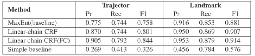
and landmarks related by a spatial pivot, we first use the disambiguated ground-truth pivots. We implemented two different classification settings. In one setting, we classify each word based on its related extracted features described in section 4.2 and using maximum entropy classifier. This process generates a multi-class classification setting in which each word is classified as trajector, landmark or none. In the second setting, we classify each word using probabilistic graphical models, particularly CRFs, considering its context (the sentence) and employing the same linguistic input features as the first setting. Tables VII and VIII show the precision, recall and F1 measures for each tag using 10-fold cross-validation on the CLEF and GUM (Maptask) datasets.
Method Trajector Pr Rec F1 Landmark Pr Rec F1 MaxEnt(baseline) 0.775 0.744 0.758 0.916 0.853 0.881 Linear-chain CRF 0.870 0.744 0.801 0.950 0.869 0.907 Linear chain CRF(FC) 0.905 0.792 0.844 0.953 0.879 0.914 Simple baseline 0.269 0.413 0.326 0.456 0.784 0.576
Table VII. Extraction of trajector/landmark roles in the CLEF dataset relying on the ground-truth preposition sense; 10-fold cross-validation.
The results show that context-dependent classification models outperform the maximum entropy model and that the differences are statistically significant forp <0.05, where the fully connected CRF model gives the best results. Using the fully connected setting of the simple tagger yields statistically significant improvements in trajector classification in CLEF and landmark classification in GUM (Maptask).
Method Trajector Pr Rec F1 Landmark Pr Rec F1 MaxEnt(baseline) 0.862 0.931 0.891 0.776 0.762 0.750 Linear-chain CRF 0.990 0.959 0.973 0.916 0.918 0.915 Linear chain CRF(FC) 1.000 0.969 0.983 0.947 1.000 0.971 Simple baseline 0.008 0.015 0.011 0.337 0.500 0.402
Table VIII. Extraction of trajector/landmark roles in the GUM (Maptask) dataset relying on the ground-truth preposition sense; 10-fold cross-validation.
5.4.2 Pipeline Setting – Exploiting Preposition Disambiguation. In this experiment,
we fully automate the tasks of recognizing spatial roles and the corresponding spatial relations. The preposition disambiguation and the extraction of trajector/landmark tasks are connected and followed by the whole-relation-extraction. The preposition classifier is trained on the TPP dataset. The landmark/trajector/none classifier is trained on the subset of GUM and also the CLEF dataset.
In this setting, various options are examined during the test phase. Each preposition in a sentence is given to the relevant classifier from the 34 TPP-classifiers. If it does not match a TPP preposition, it is an unknown preposition and treated in two distinct ways: i) nonspatial (first row in Tables IX, X) or ii) spatial (second row in the tables). If the preposition is recognized as spatial, the process of the trajector/landmark extraction is performed; otherwise, all words in the sentence are labeled as none with respect to that preposition. We compare these settings to the one in which every preposition is blindly assumed to be a spatial indicator. These results help to assess the effect of preposition disambiguation.
Training and test instances are drawn from sentences in the respective datasets. For each preposition recognized in the sentence, a distinct instance of the sentence is created. In training instances, only the landmark(s) and trajector(s) (if any) in a spatial relationship with the pivot of the instance are annotated. In test instances, trajector(s) and landmark(s) (if any) in a spatial relationship with the pivot of the instance are automatically labeled.
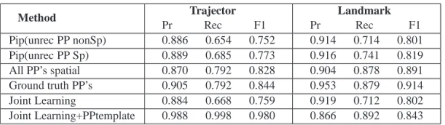
Method Trajector Pr Rec F1 Landmark Pr Rec F1 Pip(unrec PP nonSp) 0.886 0.654 0.752 0.914 0.714 0.801 Pip(unrec PP Sp) 0.889 0.685 0.773 0.916 0.741 0.819 All PP’s spatial 0.870 0.792 0.828 0.904 0.878 0.891 Ground truth PP’s 0.905 0.792 0.844 0.953 0.879 0.914 Joint Learning 0.884 0.668 0.759 0.919 0.712 0.802 Joint Learning+PPtemplate 0.988 0.998 0.980 0.866 0.892 0.843
Table IX. Extraction of trajector/landmark on CLEF dataset, comparing pipeline, ground-truth and joint learning by 10-fold cross-validation.
The experimental results in Table IX show that exploiting the linguistic features of the cor-rect spatial preposition in the CLEF corpus improves the trajector and landmark extraction performance compared to pipelining, as expected. The difference is statistically significant
(p <0.05). However, in the complete extraction problem, i.e., with unknown spatial in-dicators, assuming all prepositions to be spatial yields the highest recall, as it allows the
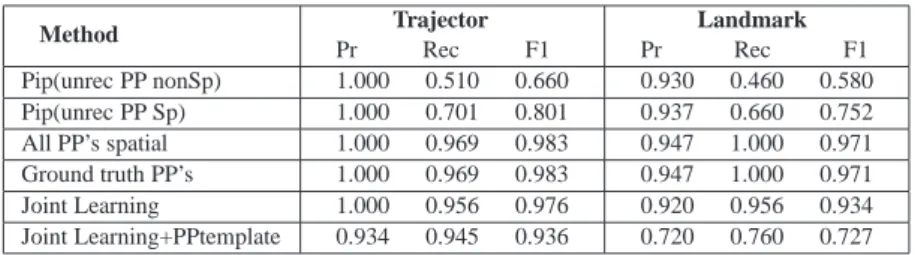
trajector/landmark classifier to find related arguments. The pipeline model (assuming un-recognized prepositions as spatial), receiving input from the preposition disambiguation module, improves precision but lowers recall. Investigating the errors indicates that no tra-jectors and landmarks are generally extracted when nonspatial prepositions are recognized as spatial and the words are correctly classified as none. However, having a spatial prepo-sition wrongly classified as nonspatial prohibits trajector and landmark extraction, causing a drop in recall. Method Trajector Pr Rec F1 Landmark Pr Rec F1 Pip(unrec PP nonSp) 1.000 0.510 0.660 0.930 0.460 0.580 Pip(unrec PP Sp) 1.000 0.701 0.801 0.937 0.660 0.752 All PP’s spatial 1.000 0.969 0.983 0.947 1.000 0.971 Ground truth PP’s 1.000 0.969 0.983 0.947 1.000 0.971 Joint Learning 1.000 0.956 0.976 0.920 0.956 0.934 Joint Learning+PPtemplate 0.934 0.945 0.936 0.720 0.760 0.727
Table X. Extraction of trajector/landmark on GUM (Maptask) dataset, comparing pipeline, ground-truth and joint learning by 10-fold cross-validation.
In the GUM (Maptask) corpus, inputting the correct preposition does not make a signifi-cant difference compared to “all spatial”; moreover, pipelining yields lower recall. GUM (Maptask)’s statistics show that more than93%of the prepositions are spatial and errors in preposition disambiguation prohibit the extraction of related trajectors and landmarks, resulting in a sharp drop in recall with no significant variation in precision.
5.4.3 Joint Learning Setting. According to section 4.3, each training instance in this
setting contains at most one preposition labeled as a spatial indicator and annotations for only the landmark(s) and trajector(s) (if any) of that spatial indicator. Each sentence gives several instances, up to the number of prepositions it contains. In test instances,
thetrajector,landmark,spatial indicatorandnonelabels are automatically assigned to
each word in the sentence based on the input features for a given preposition.
Because spatial indicators are classified jointly with other spatial roles, some of the er-rors caused by the pipelining can be removed. However, as Table IX shows on the CLEF dataset, the recall of best pipeline system (unrec PP Sp), is slightly higher than joint learn-ing in trajector and landmark classification, and the improvement is statistically significant
(p <0.1).
Adding long distance dependencies to joint learning through the preposition template greatly improves performance on CLEF dataset, particularly in trajector classification. In contrast, a sharp decrease in landmark classification occurs in GUM (Maptask). The dif-ference in language characteristics in these datasets affects these results, which calls for further investigation. In Section 5.8, an error analysis categorizes the types of errors that can occur in the spatial role labeling task and the errors of two models (with and without a template) are compared using a test subsample.
For GUM (Maptask), Table X shows that assuming all prepositions to be spatial out-performs other settings, including joint learning. The previous experiments show joint learning outperforming pipelining, though the pipeline setting uses the external resource