TESTING FOR NON-NESTED CONDITIONAL MOMENT
RESTRICTIONS VIA CONDITIONAL EMPIRICAL LIKELIHOOD
By
Taisuke Otsu and Yoon-Jae Whang
September 2005
COWLES FOUNDATION DISCUSSION PAPER NO. 1533
COWLES FOUNDATION FOR RESEARCH IN ECONOMICS
YALE UNIVERSITY
Box 208281
Testing for Non-nested Conditional Moment Retrictions
via Conditional Empirical Likelihood
∗
Taisuke Otsu
†Yale University
Yoon-Jae Whang
‡Seoul National University
September 13, 2005
Abstract
We propose non-nested tests for competing conditional moment resctriction models us-ing a method of empirical likelihood. Our tests are based on the method of conditional empirical likelihood developed by Kitamura, Tripathi and Ahn (2004) and Zhang and Gi-jbels (2003). By using the conditional implied probabilities, we develop three non-nested tests: the moment encompassing, Cox-type, and effcient score encompassing tests. Com-pared to the existing non-nested tests which mainly focus on testing unconditional moment restrictions, our approach directly tests conditional moment restrictions which imply the infinite number of unconditional moment restrictions. We derive the null distributions and power properties of the proposed tests. Simulation experiments show that our tests have reasonablefinite sample properties.
Keywords: Empirical likelihood; Non-nested tests; Encompassing tests; Cox-type tests; Con-ditional moment restrictions
JEL Codes: C12, C13, C14, C22
∗We would like to thank Yuichi Kitamura for helpful comments.
†Cowles Foundation for Research in Econonmics, Yale University, New Haven CT 06520, U.S.A. E-mail address: [email protected].
‡School of Economics, Seoul National University, Seoul 151-742, Korea. E-mail address:[email protected].
1
Introduction
Empirical econometric models are often written in the forms of conditional moment restrictions. While researchers derive and estimate their conditional moment restriction models, those models are typically nested and to be evaluated by some formal tests. This paper proposes non-nested tests for competing conditional moment restriction models using a method of empirical likelihood. Our tests are based on the method of conditional empirical likelihood (CEL) de-veloped by Kitamura, Tripathi and Ahn (2004) and Zhang and Gijbels (2003).1 By using the conditional implied probabilities from CEL, we develop three CEL-based non-nested tests: the moment encompassing, Cox-type, and efficient score encompassing tests. Compared to the exist-ing non-nested tests which mainly focus on testexist-ing parametric models or unconditional moment restrictions, our approach directly tests conditional moment restrictions which imply the infinite number of unconditional moment restrictions.
Since Cox (1961, 1962), non-nested testing for competitive statistical models has become a standard technique to evaluate specification of a statistical model against specific alternative models.2 Singleton (1985), Ghysels and Hall (1990), and Smith (1992) proposed non-nested testing procedures for unconditional moment restriction models. Recently, those procedures are extended by Ramalho and Smith (2002) to the generalized empirical likelihood (GEL) context by Smith (1997) and Newey and Smith (2004). Ramalho and Smith (2002) focused on the im-plied unconditional probabilities from the null unconditional moment restrictions, and derived GEL analogues of the moment encompassing, Cox-type, and parametric encompassing tests. We extend the approach of Ramalho and Smith (2002) to deal with conditional moment re-striction models, where the infinite number of unconditional moment rere-strictions are implied. In particular, we employ the method of CEL to obtain the conditional implied probabilities from conditional moment restrictions and derive non-nested test statistics. Since the CEL-based conditional implied probabilities contain all information from the null conditional moment re-strictions, we can directly evaluate the specification of the null model against some specific alternatives.
Since Owen (1988) and Qin and Lawless (1994), the method of empirical likelihood has
be-1Kitamura, Tripathi, and Ahn’s (2004) “smoothed” empirical likelihood and Zhang and Gijbels’ (2003) “sieve”
empirical likelihood are quite similar concepts. To avoid confusion, we introduce a new terminology, conditional empirical likelihood.
2Examples include Davidson and MacKinnon (1981), Fisher and McAleer (1981), White (1982), Gourieroux,
Monfort and Trognon (1983), Loh (1985), Mizon and Richard (1986), Wooldridge (1990), Godfrey (1998), and Chen and Kuan (2002), to mention only a few. See also Gourieroux and Monfort (1994), Pesaran and Weeks (2001) and Dhaene (1997) for a review of non-nested and encompassing tests.
come an attractive alternative against the conventional generalized method of moments (GMM) approach.3 Kitamura (2001) and Newey and Smith (2004) showed desirable properties of empir-ical likelihood for testing and estimating unconditional moment restriction models, respectively. To deal with conditional moment restriction models, Kitamura, Tripathi and Ahn (2004) and Zhang and Gijbels (2003) developed the method of CEL and showed that the CEL estimator is asymptotically efficient. Tripathi and Kitamura (2003) proposed CEL-based consistent spec-ification tests for conditional moment restrictions. This paper extends the CEL approach to non-nested testing problems. Compared to Tripathi and Kitamura’s (2003) specification tests, our tests check the validity of the null model against some specific alternatives, and our test statistics converge at the parametric rate, i.e., √n-rate. Kitamura (2003) employed CEL as a model selection criterion and proposed a Vuong (1989) type discrimination test for conditional moment restriction models, which tests whether some two competing models have the same distance (in terms of the Kullback-Leibler information criterion) from the true model. Our non-nested testing approach sets one of the competing models as the null hypothesis and checks the validity of the null model.
This paper is organized as follows. Section 2 introduces our basic setup and test statistics. In Section 3, we derive the asymptotic properties of the proposed non-nested tests. Section 4 reports simulation results. Section 5 concludes.
We use the following notation. The abbreviations “a.s.” and “w.p.a.1” mean “almost surely” and “with probability approaching one,” respectively. k·k is the Frobenius norm. A−, λ
min(A),
andλmax(A)are a g-inverse, the minimum eigenvalue, and the maximum eigenvalue of a matrix
A, respectively. I{A}is the indicator function for an eventA. int(A)is the interior of a setA.
a(i) means the i-th component of a vectora.
2
Setup and Test Statistics
2.1
Non-nested Hypotheses
Suppose that we observe a random sample{xi, zi} n
i=1, wherex∈X ⊂R
s andz
∈Rdz. Consider the two competing conditional moment restrictions:
Hg : E[g(z, β0)|x] = 0, (1) Hh : E[h(z, γ0)|x] = 0,
a.s. x, whereg :Rdz
× B→Rdg andh:Rdz
×Γ→Rdh are known functions, and β
0 ∈B⊂Rdβ
and γ0 ∈ Γ ⊂ Rdγ are unknown parameters. These conditional moment restrictions imply the
following unconditional moment restrictions:
HUg : E[Vg(x)g(z, β0)] = 0, (2) HUh : E[Vh(x)h(z, γ0)] = 0,
forany vector of measurable functionsVg andVh. Several papers such as Singleton (1985), Smith
(1992), and Ramalho and Smith (2002) proposed non-nested tests between the unconditional moment restrictions HU
g and HUh for some specific choices of Vg and Vh. However, if we are
interested in the validity of the original conditional moment restrictions Hg and Hh, the con-ventional non-nested tests for HUg and HUh may not be appropriate. For example, suppose that the true joint law satisfiesE[Vg(x)g(z, β0)] = 0butE[ ˜Vg(x)g(z, β0)]6= 0 for some function V˜g.
Then although Hg is violated, the conventional non-nested tests forHUg tend to accept the null
hypothesisHU
g. In this paper, we proposes three CEL-based non-nested tests for the conditional
moment restrictions Hg andHh.
2.2
Conditional Empirical Likelihood
This subsection introduces the CEL approach. CEL is nonparametric likelihood constructed by the conditional moment restrictions in (1). Let pgji = Pr{z =zj|x=xi} for i, j = 1, . . . , n be
multinomial conditional probabilities under the null hypothesis Hg, and wji =
Kxi−xj bn Sn j=1K xi−xj bn be Nadaraya-Watson kernel weights, where K :Rs →R is a kernel function andbn is a bandwidth
parameter. We consider the following likelihood maximization problem using pgji:
max {pgji}n i,j=1 n X i=1 n X j=1 wjilogpgji (3) s.t. pgji ≥0, n X j=1 pgji = 1, n X j=1 pgjig(zj, β) = 0, for i, j = 1, . . . , n.
The conditional moment restrictions (1) are incorporated in the constraintsPnj=1pgjig(zj, β) = 0.
This problem can be solved by the Lagrange multiplier method. Let {µgi}ni=1 and{λgi}ni=1 be the Lagrange multipliers. The Lagrangian is written as:
L= n X i=1 n X j=1 wjilogp g ji− n X i=1 µgi à n X j=1 pgji−1 ! − n X i=1 λgi0 à n X j=1 pgjig(zj, β) ! .
The solution (i.e., the implied conditional probability) is:
ˆ
pgji(β) = wji
1 +λgi (β)0g(zj, β)
, (4)
for i, j = 1, . . . , n, where λgi (β)satisfies:
n X j=1 wjig(zj, β) 1 +λgi (β)0g(zj, β) = 0, (5)
for i = 1, . . . , n. If we do not impose the conditional moment restriction Pnj=1pgjig(zj, β) = 0
in (3), the solution of the unrestricted likelihood maximization problem is pˆN
ji = wji for i, j =
1, . . . , n. Using the implied conditional probabilities {pˆgji(β)}n
i,j=1, the profile CEL function
under Hg is defined as:
g(β) = n X i=1 Iin n X j=1 wjilog ˆpgji(β) = n X i=1 Iin n X j=1 wjilog µ wji 1 +λgi (β)0g(zj, β) ¶ , (6)
where Iin =I{xi ∈Xn} with Xn⊂X is a trimming term to deal with the boundary or
denom-inator problem in the kernel estimators (see Kitamura, Tripathi and Ahn (2004, p. 1673)). The CEL estimator is defined as βˆCEL = arg maxβ∈B g(β). Kitamura, Tripathi and Ahn
(2004) showed that βˆCEL is an asymptotically normal and efficient estimator for β0 under Hg. In the same manner, we can define CEL h(γ) under Hh and the CEL estimator γˆCEL for γ0.
Kitamura (2003) showed that if Hg is misspecified, βˆCEL converges to the pseudo-true value
β∗CEL, that is
β∗CEL = arg min
β∈B E · max λg∈RdgE[log (1 +λ g0g(z, β)) |x] ¸ . (7)
The pseudo-true value γ∗CEL for γˆCEL is defined in the same manner.
To construct our non-nested test statistics, we employ some consistent estimatorsβˆandˆγfor
β0 andγ0, respectively. βˆ andγˆmay be the CEL estimators or other consistent estimators such
as the GMM estimators based on the unconditional moment restrictions in (2). Let β∗ and γ∗
be the pseudo-true values forβˆ andγˆ, respectively. Givenβˆ, the implied conditional probability underHg is obtained as{pˆgji(ˆβ)}n
i,j=1 in (4). By comparing{pˆ g
ji(ˆβ)}ni,j=1 and{pˆNji}ni,j=1, we derive
three non-nested tests: the moment encompassing, Cox-type, and efficient score encompassing tests.
To compute pˆgji(ˆβ) in (4), we need to solve n root-finding optimizations in (5) to obtain
λgi(ˆβ) for i= 1, . . . , n. However, by using an asymptotic approximation forλgi(ˆβ), we can avoid the optimizations to compute λgi(ˆβ). Since Lemma A.4 implies that λgi(ˆβ) is approximated by
˜ λgi(ˆβ) = ³Pnj=1wjig(zj,βˆ)g(zj,βˆ)0 ´−1³P n j=1wjig(zj,βˆ) ´
conditional probability is obtained as4
˜
pgji(ˆβ) = wji
1 + ˜λgi(ˆβ)0g(zj,βˆ). (8)
The non-nested test statistics based on pˆgji(ˆβ) andp˜gji(ˆβ)are asymptotically equivalent.
2.3
Test Statistics
2.3.1 Moment Encompassing Test Statistic
We first define the CEL-based moment encompassing test statistic, which focuses on the
mul-tiplicative moment indicator, m˜ (xi, zj, β, γ) = M(xi, β, γ)0m(zj, β, γ), where M(xi, β, γ) is a
dm×dM matrix of functions of xi andm(zj, β, γ)is adm×1vector of functions ofzj. A typical
choice of m˜ (xi, zj, β, γ) is M(xi, β, γ) = Idh and m(zj, β, γ) = h(zj, γ), which is based on the alternative conditional moment restrictions Hh in (1). We allowM(xi, β, γ) to be the form of
weighted sums:M(xi, β, γ) =Pnj=1wjiMz(xi, zj, β, γ). By using the implied conditional
proba-bility pˆgji(ˆβ) and the unrestricted conditional probability pˆN
ji, we consider the following contrast
of estimators for E[ ˜m(xi, zi, β0, γ∗)]: TM = 1 n n X i=1 Ii n X j=1 ˆ pgji(ˆβ) ˜m(xi, zj,β,ˆ γˆ)− 1 n n X i=1 Ii n X j=1 ˆ pNjim˜(xi, zj,β,ˆ γˆ), (9)
whereIi =I{xi ∈X∗}is a trimming term on afixed subsetX∗ ⊂X. This trimming term allows
us focus to specification testing on regions in X which are empirically more relevant. It also let us avoid the boundary problem associated with the kernel estimators, see also Tripathi and Kitamura (2003, p.2062)5. If the null hypothesis H
g is correct, TM converges to zero. If Hg is
incorrect,TM diverges in general. The moment indicatorm˜ (xi, zj, β, γ)determines the direction
of misspecification. Let ˆ Ji(β, γ)0= n X j=1 wjim(zj, β, γ)g(zj, β)0; ˆVi(β) = n X j=1 wjig(zj, β)g(zj, β)0; ˆGi(β) = n X j=1 wji∂g(zj, β)/∂β0.
The CEL-based moment encompassing test statistic forHg is defined as
Mg =nTM0 Φˆ−MTM, (10)
4>From Lemma A.1 and Assumption 3.2 (ii),Pn
j=1wjig(zj,βˆ)g(zj,ˆβ)0 is invertible w.p.a.1.
5We may also allow the trimming set to be data-dependent as in Kitamura, Tripathi, and Ahn (2004) at the
where ˆ ΦM = 1 n n X i=1 ˆ ψMi (ˆβ,γˆ)ˆψ M i (ˆβ,γˆ)0, ˆ ψMi (β, γ) = −IiM(xi, β, γ)0Jˆi(β, γ)0Vˆi(β)− 1 g(zi, β) + ˆHM(β, γ)∆ψ(xi, zi, β), ˆ HM(β, γ) = 1 n n X i=1 IiM(xi, β, γ)0Jˆi(β, γ)0Vˆi(β)−1Gˆi(β).
∆andψ(xi, zi, β) are defined in Assumption 3.1 (ii), which assumes the asymptotic linear form
for βˆ: n1/2(ˆβ−β0) =−n−1/2∆ n X i=1 ψ(xi, zi, β0) +op(1). (11)
The CEL-based moment encompassing test statistic forHh is defined in the same manner.
2.3.2 Cox-type Test Statistic
We next define the CEL-based Cox-type test statistic, which focuses on the probability limit of the GMM-type (or Euclidean) nonparametric likelihood. Let
ˆ hi(γ) = n X j=1 wjih(zj, γ) ; ˆhgi (γ) = n X j=1 ˆ pgji(ˆβ)h(zj, γ) ; ˆVih(γ) = n X j=1 wjih(zj, γ)h(zj, γ)0. By using pˆgji(ˆβ) andpˆN
ji =wji, we consider the following contrast of Euclidean likelihood:6
TC = 1 n n X i=1 Iiˆhgi (ˆγ)0Vˆ h i (ˆγ)− 1ˆ hgi (ˆγ)− 1 n n X i=1 Iiˆhi(ˆγ)0Vˆih(ˆγ)− 1ˆ hi(ˆγ). (12) LetJˆh i (β, γ)0= Pn
j=1wjih(zj, γ)g(zj, β)0. The CEL-based Cox-type test statistic forHgis defined
as Cg = √ nTC q ˆ φC , (13)
6Although we may focus on the contrast of CEL for estimatingγ
0: n X i=1 Ii n X j=1 ˆ pgji(ˆβ) log ˆphji(ˆγ)− n X i=1 Ii n X j=1 ˆ pNjilog ˆphji(ˆγ),
the asymptotic representation of the Lagrange multiplierλhi(ˆγ)inpˆhji(ˆγ)is less tractable underHg (see Kitamura (2003)). Therefore, for its simplicity, we analyze the contrast of Euclidean likelihood.
where ˆ φC = 1 n n X i=1 ˆ ψCi (ˆβ,γˆ) 2 , ˆ ψCi (β, γ) = −2Iiˆhi(γ)0Vˆih(γ)− 1 ˆ Jih(β, γ)0Vˆi(β)− 1 g(zi, β) + ˆHC(β, γ)∆ψ(xi, zi, β), ˆ HC(β, γ) = 2 n n X i=1 Iiˆhi(γ)0Vˆih(γ)− 1 ˆ Jih(β, γ)0Vˆi(β)−1Gˆi(β).
∆ andψ(xi, zi, β) are defined in (11). The CEL-based Cox-type test statistic for Hh is defined
in the same manner.
2.3.3 Efficient Score Encompassing Test Statistic
Wefinally introduce the CEL-based efficient score encompassing test statistic, which focuses on the probability limit of the asymptotic linear form of asymptotically efficient estimators for γ0
in Hh (i.e., the efficient score for estimatingγ0):7
n1/2(ˆγ−γ0) =−n−1/2Ih(γ0)− 1 n X i=1 Ghi (γ0)0Vih(γ0)− 1 h(zi, γ0) +op(1), where Vih(γ) =E£h(z, γ)h(z, γ)0|xi ¤ ; Ghi (γ) =E[∂h(z, γ)/∂γ0|xi] ; Ih(γ) =E £ Ghi (γ)0Vih(γ)−1Ghi (γ)¤. Let Gˆh i (γ) = Pn j=1wji∂h(zj, γ)/∂γ0. By using pˆ g
ji(ˆβ) and pˆNji = wji, we consider the following
contrast of the efficient score:
TS = 1 n n X i=1 IiGˆhi (ˆγ)0Vˆ h i (ˆγ)− 1ˆ hgi (ˆγ)− 1 n n X i=1 IiGˆhi (ˆγ)0Vˆ h i (ˆγ)− 1ˆ hi(ˆγ). (14)
The CEL-based efficient score encompassing test statistic is defined as
Sg =nTS0Φˆ−STS, (15)
7Although it requires a lengthy mathematical argument, we can consider the CEL-based parametric
encom-passing test statistic, which focuses on the probability limit of the CEL estimatorγˆCELforγ0. Let ˜
γCEL= arg max γ∈Γ n X i=1 Iin n X j=1 ˆ pgji(ˆβCEL) log ˆphji(γ).
Since we can expect that˜γCELis a consistent estimator for the pseudo-true valueγ∗, the CEL-based parametric
where ˆ ΦS = 1 n n X i=1 ˆ ψSi(ˆβ,ˆγ)ˆψ S i(ˆβ,γˆ)0, ˆ ψSi (β, γ) = −IiGˆih(γ)0Vˆih(γ)− 1 ˆ Jih(β, γ)0Vˆi(β)− 1 g(zi, β) + ˆHS(β, γ)∆ψ(xi, zi, β), ˆ HS(β, γ) = 1 n n X i=1 IiGˆhi (γ)0Vˆ h i (γ)− 1 ˆ Jih(β, γ)0Vˆi(β)−1Gˆi(β).
The CEL-based efficient score encompassing test statistic forHh is defined in the same manner.
2.3.4 Special Case: Test Statistics with the CEL Estimator
Suppose that we use the CEL estimator βˆCEL for β0. Then from Kitamura, Tripathi and Ahn (2004, p. 1690), we can show that under certain regularity conditions, the asymptotic linear form forβˆCEL is written as
n1/2(ˆβCEL−β0) =−n− 1/2 I(β0)− 1 n X i=1 Gi(β0)0Vi(β0)− 1 g(zi, β0) +op(1), where Gi(β) =E[∂g(z, β)/∂β0|xi] ; Vi(β) =E £ g(z, β)g(z, β)0|xi ¤ ; I(β) =E£Gi(β)0Vi(β)−1Gi(β) ¤ . By setting ∆ = I(β0)−1 and ψ(xi, zi, β0) = Gi(β0)0Vi(β0)− 1 g(zi, β0) in (10), (13), and (15),
the CEL-based non-nested test statistics are defined by the following simpler forms,
(i) the moment encompassing test statistic:
Mg,CEL =nTM0 Φˆ−M,CELTM, (16)
ˆ
ΦM,CEL=RSS for regression of Vˆi(ˆβ)−1/2Jˆi(ˆβ,γˆ)M(xi,β,ˆ γˆ) on Vˆi(ˆβ)−1/2Gˆi(ˆβ), (ii) the Cox-type test statistic:
Cg,CEL= √ nTC q ˆ φC,CEL , (17) ˆ
φC,CEL =RSS for regression of 2 ˆVi(ˆβ)−1/2Jˆih(ˆβ,γˆ) ˆV h i (ˆγ)−
1ˆh
i(ˆγ) on Vˆi(ˆβ)−1/2Gˆi(ˆβ),
(iii) the efficient score encompassing test:
Sg,CEL=nTS0Φˆ−S,CELTS, (18)
ˆ
ΦS,CEL=RSS for regression of Vˆi(ˆβ)−1/2Jˆih(ˆβ,ˆγ) ˆV h i (ˆγ)−
1Gˆh
i(ˆγ) onVˆi(ˆβ)−1/2Gˆi(ˆβ),
The asymptotic properties obtained in the next section hold for the above test statistics as well. The above formulae are also applicable to other semiparametric efficient estimators by Newey (1990) and Donald, Imbens and Newey (2003) for example.
3
Asymptotic Properties
3.1
Null Distributions
In this subsection, we derive the asymptotic distributions of the CEL-based non-nested test statistics under the null hypothesisHg. We impose the following assumptions.
Assumption 3.1
(i) {xi, zi}
n
i=1 is an i.i.d. sample on X ×R
dz, x is continuously distributed with density f,
X∗
is compact and contained inint(X), and infx∈X∗f(x)>0.
(ii) β0 ∈int(B), and βˆ satisfies n1/2(ˆβ
−β0) =−n−1/2∆Pn
i=1ψ(xi, zi, β0) +op(1), where ∆ is
a dβ×dβ non-stochastic matrix, E[ψ(x, z, β0)] = 0, and E[||ψ(x, z, β0)||ξ] <∞ for some
ξ >2.
(iii) kγˆ−γ∗k=Op(n−1/2).
(iv) K(x) =Πsi=1κ(x(i)), where κ is a continuously differentiable pdf with support[−1,1],
sym-metric around the origin, and infx∈[−k,¯¯k]κ(x)>0 for some k¯∈(0,1).
(v) bn=n−α for 0< α <minn1 3s, 1 s ³ 1− 4 ζ ´ ,1 s ³ 1− 4 ζm ´ ,1 s ³ 1− 2 ζ − 2 η ´ ,1 s ³ 1− 2 ζm − 2 η ´ ,1 s ³ 1− 2 ζ − 2 ηm ´o . Assumption 3.2
(i) E[supβ∈Bkg(z, β)kζ]<∞ for some ζ ≥6.
(ii) f(x)andE[g(z, β0)g(z, β0)0|x]are twice continuously differentiable onX,E[∂g(z, β0)/∂β0|x]
is continuous on X,f(x) and E[kg(z, β0)k ζ
|x]f(x) are uniformly bounded onX, and
infx∈X∗λmin(E[g(z, β0)g(z, β0)0|x])>0.
(iii) g(z, β) is twice continuously differentiable a.s. on a neighborhood B0 around β0, for i =
1, . . . , dg and j = 1, . . . , dβ, supβ∈B0|∂g
(i)(z, β)/∂β(j)
| ≤ d1(z) holds a.s. for a
real-valued function d1(z) with E[d1(z) η
] < ∞ for some η ≥ 6, and for i = 1, . . . , dg and
j, k = 1, . . . , dβ, supβ∈B0|∂
2g(i)(z, β)/∂β(j)∂β(k)
| ≤ d2(z) holds a.s. for a real-valued
(iv) supx∈X∗||M(x,β,ˆ γˆ) − M¯ (x, β0, γ∗)||
p
→ 0, M¯ (x, β0, γ∗) is uniformly bounded on X∗,
E[supβ∈B,γ∈Γkm(z, β, γ)k
ζm
] < ∞ for some ζm ≥ 6, m(z, β, γ) is continuously diff
er-entiable a.s. on a neighborhood B0 × Γ∗ around (β0, γ∗), and for i = 1, . . . , dm and
j = 1, . . . , dβ +dγ, sup(β,γ)∈B0×Γ∗|∂m
(i)(z, β, γ)/∂(β0, γ0)(j)| ≤ d
m(z) holds a.s. for a
real-valued function dm(z) with E[dm(z)ηm]<∞ for some ηm ≥6.
In Assumption 3.1 (i), although x should be continuous, z can be continuous, discrete, or mixed. Assumption 3.1 (ii) assumes the asymptotic linear form for βˆ and implies the asymp-totic normality of βˆ. This assumptions holds for a number of parametric and semiparametric estimators. Assumption 3.1 (iii) imposes the √n-consistency of ˆγ to the pseudo-true value γ∗. Depending on the estimation method, γ∗ may be different. Assumption 3.1 (iv) and (v) are conditions for the kernel function K and the bandwidth bn. Assumption 3.1 (iv) rules out
ker-nel functions whose orders are higher than two. Assumption 3.2 (i)-(iii) are conditions for the moment function g(z, β), which are mainly used to derive the convergence of nonparametric components such asVˆi(ˆβ)andGˆi(ˆβ). Assumption 3.2 (iv) is a set of conditions for the moment
indicatorm˜ (x, z, β, γ). For the Cox-type and efficient score encompassing test statistics, we take
m(zi, β, γ) =h(z, γ). Let Jh i (β, γ)0=E £ h(z, γ)g(z, β)0|xi ¤
. The null distributions of the CEL-based non-nested test statistics are obtained as follows.
Theorem 3.1 (Null Distributions)
(i) Suppose that Assumptions 3.1 and 3.2 hold. Then under the null hypothesis Hg,
Mg d
→χ2rank(ΦM),
whereΦM (defined below (41)) is the probability limit of ΦˆM.
(ii) Suppose that Assumptions 3.1 and 3.2 (i)-(iii) hold, and Assumption 3.2 (iv) holds for
m(zi, β, γ) =h(zi, γ), M(xi, β, γ)0 ={2ˆhi(γ)−Jih(β, γ) ˆVi(β)−1ˆgi(β)}0Vˆih(γ)−1, and
¯
Mi(xi, β, γ)0 = 2E[h(z, γ)|xi]0Vih(γ)− 1
. Then under the null hypothesis Hg,
Cg d
→N(0,1).
(iii) Suppose that Assumptions 3.1 and 3.2 (i)-(iii) hold, and Assumption 3.2 (iv) holds for
m(zi, β, γ) =h(zi, γ),Mi(xi, β, γ)0 = ˆGhi (γ)0Vˆih(γ)− 1
, andM¯i(xi, β, γ)0 =Ghi(γ)0Vih(γ)− 1
. Then under the null hypothesis Hg,
Sg d
→χ2rank(ΦS),
Therefore, all the non-nested test statistics follow the standard limiting distributions. Com-pared to the CEL-based specification test statistics by Tripathi and Kitamura (2003), our non-nested test statistics show the parametric convergence rate. For (ii) and (iii) of this theorem, the assumptions on m(zi, β, γ)andM(xi, β, γ)can be replaced with more primitive conditions,
such as the conditions obtained by replacing g(z, β), β0, B, and B0 in Assumption 3.2 (i)-(iii)
with h(z, γ),γ∗,Γ, and Γ∗, respectively.
3.2
Power Properties
This subsection studies the power properties of the CEL-based non-nested test statistics under some local alternative hypothesis. We assume that the joint distribution of (x, z) is fixed, and that there exists a nonstochastic sequenceβ0n ∈B such that
Hgn :E[g(z, β0n)|x] =n−1/2δ(x) (19)
holds a.s. for some δ : X → Rdg. The null hypothesis H
g is satisfied if δ(x) = 08. We impose
the following assumptions.
Assumption 3.3
(i) δ(x) is continuous on X , E[kδ(x)kζ] <∞, kβ0n−β0k→ 0 as n→ ∞, β0 ∈ int(B), and
n1/2(ˆβ−β0n) =−n−1/2∆
Pn
i=1ψ(xi, zi, β0n) +op(1), where ∆ is a dβ×dβ non-stochastic
matrix,E[ψ(x, z, β0n)|x] =n−1/2δψ(x),δψ(x)is continuous onX, andE[kδψ(x)k ζ
]<∞.
(ii) f(x) and E[g(z, β)g(z, β)0|x] are twice continuously differentiable on X for each β ∈B0,
E[g(z, β)g(z, β)0|x] and E[∂g(z, β)/∂β0|x] are continuous on X × B0, f(x) and
supβ∈B0E[kg(z, β)kζ|x]f(x) are uniformly bounded onX,
inf(x,β)∈X∗×B0λmin(E[g(z, β)g(z, β)
0
|x])>0, andinf(x,β)∈X∗×B0λmax(E[g(z, β)g(z, β)
0
|x])<
∞.
(iii) supx∈X∗||M(x,β,ˆ γˆ)−M¯ (x, β0n, γ∗)||
p
→ 0, supβ∈B0M¯ (x, β, γ∗) is uniformly bounded on
X∗, E[supβ∈B,γ∈Γkm(z, β, γ)k
ζm] <
∞ for some ζm ≥ 6, m(z, β, γ) is continuously
dif-ferentiable a.s. on a neighborhood B0 ×Γ∗ around (β0, γ∗), and for i = 1, . . . , dm and 8Another way to formulate the local alternatives in the spirit of Singleton (1985, p.402) would be
H∗gn: µ 1−√η n ¶ E[g(z, β0)|x] +√η nE[h(z, γ)|x] = 0,
where η ∈ R is a constant. This case can be treated similarly because H∗
gn now corresponds to Hgn with δ(x) =η{E[g(z, β0)|x]−E[h(z, γ)|x]}andβ0n =β0.
j = 1, . . . , dβ +dγ, sup(β,γ)∈B0×Γ∗|∂m
(i)(z, β, γ)/∂(β0, γ0)(j)| ≤ d
m(z) holds a.s. for a
real-valued function dm(z) with E[dm(z) ηm]<
∞ for some ηm ≥6.
Assumption 3.3 (i), (ii), and (iii) are extensions of Assumptions 3.1 (ii) and 3.2 (ii) and (iv), respectively. Let Ji(β, γ)0=E[m(z, β, γ)g(z, β)0|xi], and χ2d(v) be the noncentral chi-squared
distribution with the degree of freedom d and the noncentrality parameter v. The local power properties of the CEL-based non-nested test statistics are obtained as follows.
Theorem 3.2 (Local Power)
(i) Suppose that Assumptions 3.1 (i) and (iii)-(v), 3.2 (i) and (iii), and 3.3 hold. Then under the local alternative hypothesis Hgn,
Mg d →χ2rank(ΦM) ¡ µ0MΦ−MµM ¢ , where µM =−E £ IiM(xi, β0, γ∗)0Ji(β0, γ∗)0Vi(β0)− 1 δ(xi) ¤ +HM(β0, γ∗)∆E[δψ(xi)], HM(β, γ) =E £ IiM(xi, β, γ)0Ji(β, γ)0Vi(β)−1Gi(β) ¤ .
(ii) Suppose that Assumptions 3.1 (i) and (iii)-(v), 3.2 (i) and (iii), and 3.3 (i)-(ii) hold, and Assumption 3.3 (iii) holds for m(zi, β, γ) =h(zi, γ), M(xi, β, γ)0 =
{2ˆhi(γ) − Jih(β, γ) ˆVi(β)−1gˆi(β)}0Vˆih(γ)−1, and M¯i(xi, β, γ)0 = 2E[h(z, γ)|xi]0Vih(γ)− 1
. Then under the local alternative hypothesis Hgn,
Cg d →N³φ−C1/2µC,1´, where µC =−2E £ IiE[h(z, γ∗)|xi]0Vih(γ∗)− 1 Jih(β0, γ∗)0Vi(β0)− 1 δ(xi) ¤ +HC(β0, γ∗)∆E[δψ(xi)], HC(β, γ) =2E £ IiE[h(z, γ)|xi]0Vih(γ)− 1 Jih(β, γ)0Vi(β)−1Gi(β) ¤ .
(iii) Suppose that Assumptions 3.1 (i) and (iii)-(v), 3.2 (i) and (iii), and 3.3 (i)-(ii) hold, and
Assumption 3.3 (iii) holds for m(zi, β, γ) =h(zi, γ), Mi(xi, β, γ)0 = ˆGhi (γ)0Vˆih(γ)− 1
, and
¯
Mi(xi, β, γ)0 =Gih(γ)0Vih(γ)− 1
. Then under the local alternative hypothesis Hgn,
Sg d →χ2rank(ΦS)¡µ0SΦ−SµS¢, where µS =−E£IiGhi (γ∗)0V h i (γ∗)− 1 Jih(β0, γ∗)0Vi(β0)− 1 δ(xi) ¤ +HS(β0, γ∗)∆E[δψ(xi)], HS(β, γ) =E £ IiGhi (γ)0V h i (γ)− 1 Jih(β, γ)0Vi(β)−1Gi(β) ¤ .
Therefore, similar to the conventional non-nested tests, the local power functions are obtained from the standard noncentral distributions. While the CEL-based specification test by Tripathi and Kitamura (2003) has non-trivial power against the local alternatives with a nonparametric rate (i.e., n−1/2b−s/4
n δ(x)), our CEL-based non-nested tests have non-trivial power against the
local alternatives with the parametric rate (i.e.,n−1/2δ(x)). For (ii) and (iii) of this theorem, we
can also replace the assumptions onm(zi, β, γ) andM(xi, β, γ)with more primitive conditions,
such as the conditions obtained by replacing g(z, β), β0, B, and B0 in Assumptions 3.2 (i) and
(iii) and 3.3 (ii) with h(z, γ), γ∗, Γ, and Γ∗, respectively.
We finally derive the consistency of the CEL-based non-nested tests under the alternative
hypothesis Hh. We assume that under Hh the estimators βˆ andγˆ converge to the pseudo-true
valuesβ∗ andγ0, respectively. Let B∗ and Γ0 be neighborhoods around β∗ andγ0, respectively, and
λg∗(x, β) = arg max
λ∈Rdg
E[log (1 +λ0g(z, β))|x].
>From Kitamura (2003), we have maxi∈I∗||λgi(ˆβ)−λ g ∗(xi, β∗)|| p →0 underHh. Let Ji∗(β, γ)0 = E · m(z, β, γ)g(z, β)0 1 +λg∗(xi, β)0g(z, β) ¯ ¯ ¯ ¯xi ¸ , Jih∗(β, γ)0 =E · h(z, γ)g(z, β)0 1 +λg∗(xi, β)0g(z, β) ¯ ¯ ¯ ¯xi ¸ , ˆ Jih∗(β, γ)0 = n X j=1 wji h(zj, γ)gj(β)0 1 +λgi(β)0gj(β).
The consistency results are obtained as follows.
Theorem 3.3 (Consistency)
(i) Suppose that for β∗, γ0, B∗, and Γ0 instead of β0, γ∗, B0, and Γ∗, respectively,
Assump-tions 3.1 and 3.2 hold. Then under the alternative hypothesis Hh, the CEL-based moment encompassing test by Mg is consistent if µ0hMΦ−hMµhM >0, where
µhM =−E£IiM¯i(xi, β∗, γ0)0Ji∗(β∗, γ0)0λ g
∗(xi, β∗)
¤
,
and ΦhM is the probability limit of ΦˆM under Hh.
(ii) Suppose that for β∗, γ0, B∗, and Γ0 instead of β0, γ∗, B0, and Γ∗, respectively,
Assump-tions 3.1 and 3.2 (i)-(iii) hold, and Assumption 3.2 (iv) holds for m(zi, β, γ) = h(zi, γ),
M(xi, β, γ)0 =nPnj=1wji 2h(zj,γ) 1+λgi(β)0gj(β) + ˆJih∗(β, γ)0λ g i(β) o0 ˆ Vh i (γ)− 1 , andM¯i(xi, β, γ)0 = n Eh 2h(z,γ0) 1+λg∗(xi,β∗)0g(z,β∗) ¯ ¯ ¯xi i +Jh i∗(β∗, γ0)0λ g ∗(xi, β∗) o0 Vh i (γ0)− 1
. Then under the alternative hypothesis Hh, the CEL-based Cox-type test by Cg is consistent if µ2hC/φhC >0, where
µhC = −E[Ii ½ E · 2h(z, γ0) 1 +λg∗(xi, β∗)0g(z, β∗) ¯ ¯ ¯ ¯xi ¸ +Jih∗(β∗, γ0)0λg∗(xi, β∗) ¾0 ×Vih(γ0)−1Jih∗(β∗, γ0)0λg∗(xi, β∗)],
and φhC is the probability limit ofφˆhC under Hh.
(iii) Suppose that for β∗, γ0, B∗, and Γ0, instead of β0, γ∗, B0, and Γ∗, respectively,
Assump-tions 3.1 and 3.2 (i)-(iii) hold, and Assumption 3.2 (iv) holds for m(zi, β, γ) = h(zi, γ),
Mi(xi, β, γ)0 = ˆGhi (γ)0Vˆih(γ)− 1
, andM¯i(xi, β, γ)0 =Ghi(γ)0Vih(γ)− 1
. Then under the alter-native hypothesisHh, the CEL-based efficient score test bySg is consistent ifµ0hSΦ−hSµhS >
0, where µhS =−E £ IiGhi (γ0)0Vih(γ0)− 1 Jih∗(β∗, γ0)0λ g ∗(xi, β∗) ¤ ,
and ΦhS is the probability limit of ΦˆS under Hh.
4
Simulations
This section examines the finite sample properties of our tests against some of the existing non-nested tests using Monte-Carlo methods.
4.1
Experimental Design
We consider two simulation designs. In Design I, we consider two competing linear regression models: for i= 1, ..., n,
Hg : yi =β01+β02x1i+ugi (20)
Hh : yi =γ01+γ02x2i+uhi,
where x1i =c0x2i+ei for c0 ∈{1,2},{x2i} and {ei} are i.i.d. N(0,1), {ugi} and {uhi} are i.i.d.
N(0,4), and the true parameters are given by β0 = (β01, β02)0 = (1,1)0 and γ
0 = (γ01, γ02)0 =
(1,1)0. Note that the hypotheses (20) correspond to the conditional moment restrictions in (1) with g(z, β0) = y −β01 −β02x1 and h(z, γ0) = y −γ01 −γ02x2, where z = (y, x1, x2)0 and
x= (x1, x2)0.
On the other hand, in Design II, we consider the following regression models: fori= 1, ..., n,
Hg : yi =β0xi+ugi (21)
Hh : yi =γ0x3i +uhi,
where{xi},{ugi}and {uhi}are i.i.d. N(0,1)andβ0 =γ0 = 1. The hypotheses (21) correspond
to (1) with g(z, β0) =y−β0x andh(z, γ0) =y−γ0x3,where z = (y, x)0.
As benchmarks for our simulation experiments, we consider the non-nested tests of Singleton (1985, eqn. (33), p.404), labelled S,and Ramalho and Smith (2002, Simplified Cox test in Eqn.
(4.4), p.108), labelledSC,respectively. We computeS andSC from the following unconditional moment restrictions implied by (20) and (21): for Design I,
HUg : E[(1, x1i, x2i)0(yi−β01−β02x1i)] = 0 (22) HUh : E[(1, x1i, x2i)0(yi−γ01−γ02x2i)] = 0
and, for Design II,
HUg : E[(1, xi)0(yi−β0xi)] = 0 (23) HUh : E£(1, xi3)0¡yi−γ0x 3 i ¢¤ = 0.
As another benchmark, we also consider the over-identifying test of Hansen (1982), labelled J,
that tests the validity ofHUg in (22) and (23) against general alternatives.
We consider two sample sizesn∈{100,200}andfix the numberRof Monte Carlo repetitions to be1000.Because of very long computing time required for nonlinear optimizations, we do not consider larger n and R. We use the Gaussian kernel for our CEL-based tests Mg, Cg, andSg.
For the bandwidthbn, we consider bn∈[0.1,0.2, ...,1.0]in our simulations.
4.2
Simulation Results
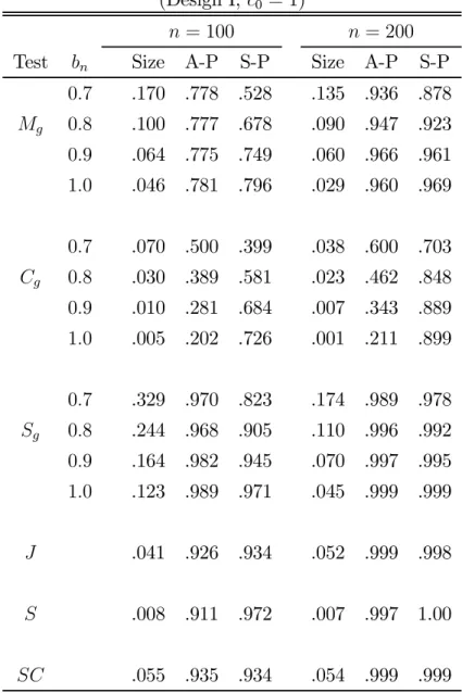
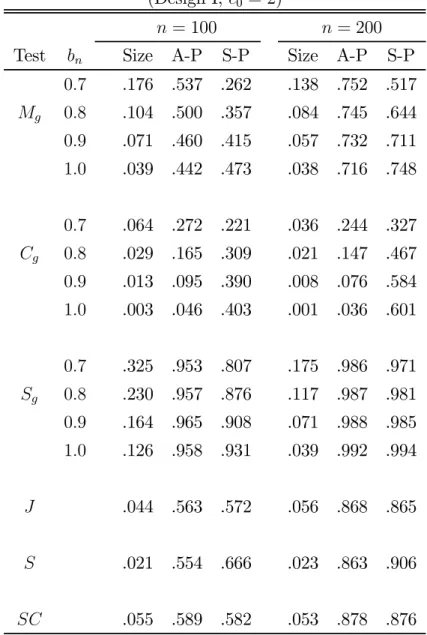
Tables 1-3 present the rejection probabilities for the tests with nominal size of5%.The simulation standard errors are approximately 0.007. Tables 1 and 2 give the results for Design I with
c0 = 1 and c0 = 2, respectively. In both cases, our tests have reasonable size performance if
the bandwidth is in a suitable range. The performance improves generally as n increases. The competitorsJ andSC also have little size distortions, though the Singleton’s testSunder-rejects in many cases we consider. In terms of size-corrected powers, the efficient score encompassing test Sg dominates Mg and Cg in Design I. When c0 = 1, the test S which is known to have
an optimality property against some local alternatives, has relatively very good (size-corrected) power performance. However, when c0 = 2, the power performance of S deteriorates and is
significantly dominated by that of Sg. To explain the latter phenomenon, notice that if the
alternative hypothesis Hh in (20) is true, then the GMM estimator bβ = (βb1,βb2)0 converges
(in probability) to the pseudo-true value β∗ = (1, c0/(1 +c20))0 . This implies that the sample
analogue of the unconditional expectation in (22) converges
1 n n X i= h (1, x1i, x2i)0 ³ yi−bβ1−bβ2x1i ´i p → µ 0,0, 1 1 +c2 0 ¶0 . (24)
Therefore, since the limit in (24) degenerates to zero asc0 increases, we can see that a test based
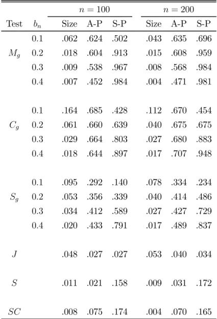
Table 3 reports the simulation results for Design II. In this design, we expect that the tests based on the unconditional moments in (23) will be inconsistent. It is because, under Hh, the
estimator βb converges in probability to the pseudo-true value β∗ = 3 and hence the sample average converges to 1 n n X i= h (1, xi)0 ³ yi−bβxi ´i p →EH[(1, xi)0(yi−β∗xi)] = (0,0)0, (25)
where EH is the expectation taken under Hh. This is precisely what happens to the powers of
the tests J, S, andSC in Design II. On the other hand, our tests have non-trivial powers even in this case. Among the latter tests, Mg and Cg appear to have better (size-corrected) power
performance thanSg in this design.
5
Conclusion
We propose three non-nested tests for competing conditional moment restriction models. Our test statistics are based on the implied conditional probabilities by conditional empirical like-lihood. The proposed tests (the moment encompassing, Cox-type, and efficient score encom-passing tests) follow the standard limiting distributions. Simulation results illustrate that our non-nested tests have reasonable finite sample properties and, in some cases, dominate some of the existing tests based on unconditional moment restrictions.
A
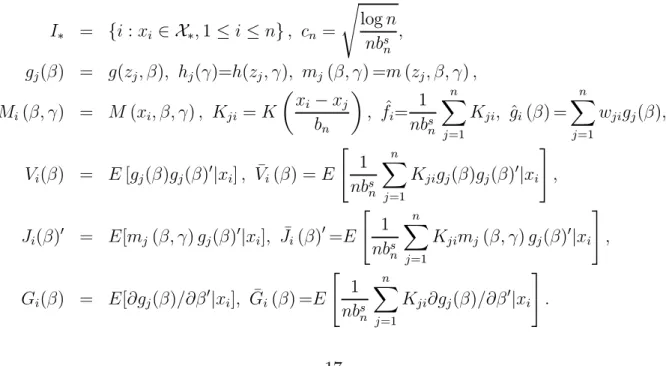
Mathematical Appendix
Notation. Denote I∗ = {i:xi ∈X∗,1≤i≤n}, cn= s logn nbs n , gj(β) = g(zj, β), hj(γ)=h(zj, γ), mj(β, γ) =m(zj, β, γ), Mi(β, γ) = M(xi, β, γ), Kji =K µ xi−xj bn ¶ , fˆi= 1 nbs n n X j=1 Kji, gˆi(β) = n X j=1 wjigj(β), Vi(β) = E[gj(β)gj(β)0|xi], V¯i(β) =E " 1 nbs n n X j=1 Kjigj(β)gj(β)0|xi # , Ji(β)0 = E[mj(β, γ)gj(β)0|xi], J¯i(β)0=E " 1 nbs n n X j=1 Kjimj(β, γ)gj(β)0|xi # , Gi(β) = E[∂gj(β)/∂β0|xi], G¯i(β) =E " 1 nbs n n X j=1 Kji∂gj(β)/∂β0|xi # .A.1
Proof of Theorem 3.1
Proof of (i) An expansion of pˆgji(ˆβ) aroundλ g i(ˆβ) = 0 yields ˆ pgji(ˆβ) = wji 1 +λgi(ˆβ)0gj(ˆβ) =wji ³ 1−λgi(ˆβ)0gj(ˆβ) +rji ´ , (26) where rji = λgi(ˆβ)0gj(ˆβ)gj(ˆβ)0λg i(ˆβ) (1+˜λgi0gj(ˆβ))3 , and ˜λgi is a point on the line joining λgi(ˆβ)and 0. Since pˆgji(ˆβ)− ˆ
pNji =wji
³
−λgi(ˆβ)0gj(ˆβ) +rji
´
, the definition of TM in (9) implies
TM = − 1 n n X i=1 IiMi(ˆβ,γˆ)0Jˆi(ˆβ,ˆγ)0λgi(ˆβ) + 1 n n X i=1 IiMi(ˆβ,ˆγ)0 Ã n X j=1 wjirjimj(ˆβ,ˆγ) ! (27) = T(1)+R(1). R(1) satisfies ° °R(1)°°≤max i∈I∗ ° ° °Mi(ˆβ,γˆ) ° ° ° max 1≤j≤n ° ° °mj(ˆβ,γˆ) ° ° ° µ max i∈I∗ ° ° °λgi(ˆβ) ° ° ° ¶2°° ° ° ° 1 n n X i=1 Ii n X j=1 wji gj(ˆβ)gj(ˆβ)0 (1 + ˜λgi0gj(ˆβ))3 ° ° ° ° °. (28) Assumption 3.2 (iv) implies
max i∈I∗ ° ° °Mi(ˆβ,γˆ) ° ° °=Op(1). (29)
>From Assumption 3.2 (i) and (iv) and Tripathi and Kitamura (2004, Lemma C.4),
max 1≤j≤n ° ° °gj(ˆβ) ° ° °=o¡n1/ζ¢, max 1≤j≤n ° ° °mj(ˆβ,γˆ) ° ° °=o¡n1/ζm¢. (30) >From Lemmas A.1 and A.4,
max i∈I∗ ° ° °λgi(ˆβ) ° ° °=Op(cn) +op ³ n−12+ 1 η ´ . (31)
Since (30) and (31) imply thatmaxi∈I∗,1≤j≤n|˜λ
g0 i gj(ˆβ)|=op(1), we have ° ° ° °1n Pn i=1Ii Pn j=1wji gj(ˆβ)gj(ˆβ)0 (1+˜λgi0gj(ˆβ)) 3 ° ° °
°≤Op(1) by Lemma A.1. Thus, from (28)-(31),
° °R(1)°°≤Op(1)o ¡ n1/ζm¢ nO p(cn) +op ³ n−12+ 1 η ´o2 Op(1) =op ¡ n−1/2¢, (32) where the equality follows from α < 1s³1− ζ4
m ´ and ζ1 m + 2 η ≤ 1
2. >From (27) and Lemma A.4,
TM = − 1 n n X i=1 IiMi(ˆβ,γˆ)0Jˆi(ˆβ,γˆ)0Vˆi(ˆβ)−1gˆi(ˆβ)− 1 n n X i=1 IiMi(ˆβ,ˆγ)0Jˆi(ˆβ,γˆ)0rig+op ¡ n−1/2¢ = T(2)+R(2)+op ¡ n−1/2¢. (33)
>From (29) and Lemmas A.2 and A.4, R(2) satisfies ° °R(2)°° ≤ max i∈I∗ ° ° °Mi(ˆβ,γˆ) ° ° °max i∈I∗ kr g ik ° ° ° ° ° 1 n n X i=1 IiJˆi(ˆβ,ˆγ) ° ° ° ° ° = Op(1)op ¡ n1/ζ¢ nOp ¡ c2n¢+op ³ n−1+2η ´o Op(1) = op ¡ n−1/2¢, (34) where the last equality follows fromα < 1s³1− 4ζ´ and 1ζ +η2 ≤ 12. Thus, from (33),
TM = − 1 n n X i=1 IiMi(ˆβ,γˆ)0Jˆi(ˆβ,ˆγ)0Vˆi(ˆβ)−1gˆi(ˆβ) +op ¡ n−1/2¢ = −1 n n X i=1 IiM¯i(β0, γ∗)0Jˆi(β0, γ∗)0Vˆi(β0)− 1 ˆ gi(ˆβ) +R(3)+op ¡ n−1/2¢. (35)
R(3) is implicitly defined and satisfies
||R(3)|| ≤ ° ° ° ° ° 1 n n X i=1 Ii{Mi(ˆβ,γˆ)−M¯i(β0, γ∗)}0Jˆi(ˆβ,γˆ)0Vˆi(ˆβ)−1gˆi(ˆβ) ° ° ° ° ° + ° ° ° ° ° 1 n n X i=1 IiM¯i(β0, γ∗)0{Jˆi(ˆβ,ˆγ)−Jˆi(β0, γ∗)}0Vˆi(ˆβ)−1gˆi(ˆβ) ° ° ° ° ° + ° ° ° ° ° 1 n n X i=1 IiM¯i(β0, γ∗)0Jˆi(β0, γ∗)0{Vˆi(ˆβ)−1−Vˆi(β0)−1}ˆgi(ˆβ) ° ° ° ° ° = ||R(3)a ||+||Rb(3)||+||Rc(3)||.
>From Assumption 3.2 (iv) and a similar argument to derive (40) shown below, we have||R(3)a ||=
op
¡
n−1/2¢. Assumption 3.2 (iv) and Lemmas A.1, A.2, and A.4 yield
||R(3)b || ≤ max i∈I∗ || ¯ Mi(β0, γ∗)||maxi∈I ∗ || ˆ Ji(ˆβ,ˆγ)−Jˆi(β0, γ∗)||maxi∈I ∗ || ˆ Vi(ˆβ)−1|| ° ° ° ° ° 1 n n X i=1 Iigˆi(ˆβ) ° ° ° ° ° = Op(1) n op ³ n−12+ 1 ζm+ 1 η ´ +op ³ n−12+ 1 ζ+ 1 ηm ´o Op(1) n Op(cn) +op ³ n−12+ 1 η ´o =op ¡ n−1/2¢,
where the last equality follows from ζ1 m + 2 η ≤ 1 2, 1 ζ + 1 ηm + 1 η ≤ 1 2, and Assumption 3.1 (v).
Similarly, Assumption 3.2 (iv) and Lemmas A.1, A.2, and A.4 imply that ||R(3)b || =op
¡
Thus, from (35), TM = − 1 n n X i=1 IiM¯i(β0, γ∗)0Jˆi(β0, γ∗)0Vˆi(β0)− 1 ˆ gi(ˆβ) +op ¡ n−1/2¢ = −1 n n X i=1 IiM¯i(β0, γ∗)0Jˆi(β0, γ∗)0Vˆi(β0)− 1 {gˆi(β0) + ˆGi(˜β)(ˆβ−β0)}+op ¡ n−1/2¢ = −1 n n X i=1 IiM¯i(β0, γ∗)0Jˆi(β0, γ∗)0Vˆi(β0)− 1 ˆ gi(β0) + ˆHM(β0, γ∗)∆ 1 n n X i=1 ψ(xi, zi, β0) +R(4)+op ¡ n−1/2¢ = TM a+TM b+R(4)+op ¡ n−1/2¢, (36)
where the second equality follows from an expansion of gˆi(ˆβ) around βˆ =β0, and β˜ is a point
on the line joining βˆ andβ0. R(4) is implicitly defined and satisfies ° °R(4)°° ≤ ° ° ° ° ° 1 n n X i=1 IiM¯i(β0, γ∗)0Jˆi(β0, γ∗)0Vˆi(β0)− 1 {Gˆi(˜β)−Gˆi(β0)} ° ° ° ° °||βˆ−β0|| + ° ° ° ° ° 1 n n X i=1 IiM¯i(β0, γ∗)0Jˆi(β0, γ∗)0Vˆi(β0)− 1 ˆ Gi(β0) ° ° ° ° °op ¡ n−1/2¢ ≤ max i∈I∗ || ¯ Mi(β0, γ∗)||maxi∈I ∗ || ˆ Ji(β0, γ∗)||maxi∈I ∗ || ˆ Vi(β0)−1|| ° ° ° ° ° 1 n n X i=1 Ii{Gˆi(˜β)−Gˆi(β0)} ° ° ° ° °||βˆ−β0|| + max i∈I∗ || ¯ Mi(β0, γ∗)||maxi∈I ∗ || ˆ Ji(β0, γ∗)||maxi∈I ∗ || ˆ Vi(β0)− 1 ||max i∈I∗ || ˆ Gi(β0)||op ¡ n−1/2¢ = op ³ n−1+η12 ´ +op ¡ n−1/2¢=op ¡ n−1/2¢,
where the equality follows from Assumption 3.2 (iv) and Lemmas A.1, A.2, and A.3. Thus, from (36), we haveTM =TM a+TMb+op ¡ n−1/2¢. T M a is written as TM a = − 1 n n X i=1 n X j=1 IiE[ ˆfi|xi]−1M¯i(β0, γ∗)0J¯i(β0, γ∗)0V¯i(β0)− 1 1 nbs n Kjigj(β0) +R(5)a = T¯M a+R(5)a , (37)
where R(5)a is implicitly defined and satisfies
° °R(5)a °° ≤ ° ° ° ° ° 1 n n X i=1 IiM¯i(β0, γ∗)0 n ˆ Ji(β0, γ∗)−E[ ˆfi|xi]−1J¯i(β0, γ∗) o0 ˆ Vi(β0)− 1 ˆ gi(β0) ° ° ° ° ° + ° ° ° ° ° 1 n n X i=1 IiE[ ˆfi|xi]−1M¯i(β0, γ∗)0J¯i(β0, γ∗)0 n ˆ Vi(β0)− 1 −E[ ˆfi|xi] ¯Vi(β0)− 1o ˆ gi(β0) ° ° ° ° ° + ° ° ° ° ° 1 n n X i=1 n X j=1 Ii n ˆ fi−1−E[ ˆfi|xi]−1 o ¯ Mi(β0, γ∗)0J¯i(β0, γ∗)0V¯i(β0)− 1 1 nbs n Kjigj(β0) ° ° ° ° ° = ||R(5)aa||+||R(5)ab||+||R(5)ac||.
>From Assumption 3.2 (iv), Lemmas A.1 and A.2, and Tripathi and Kitamura (2004, Lemma C.1), we have ||R(5)aa||≤Op(c2n) =op(n−1/2)from α < 31s. Similarly, we have ||R
(5)
ab ||≤Op(c2n) =
op(n−1/2). Moreover, Assumption 3.2 (iv), Lemmas A.1 and A.2, and Tripathi and Kitamura
(2004, eqn. (C.1)) imply ||R(5)ac|| ≤ Op(c2n) = op(n−1/2). Thus, from (37), we have TM a =
¯
TM a+op
¡
n−1/2¢. By applying the U-statistic arguments of Kitamura, Tripathi and Ahn (2004,
pp.1696-1698) and Powell, Stock and Stoker (1989, Lemma 3.1), we have the asymptotic linear forms forT¯M a: n1/2T¯M a =−n−1/2 n X i=1 IiM¯i(β0, γ∗)0Ji(β0, γ∗)0Vi(β0)− 1 gi(β0) +op(1). (38)
>From Lemmas A.1, A.2, and A.3, and a weak law of large numbers, we can show that
ˆ HM(β0, γ∗) p →E[IiM¯i(β0, γ∗)0Ji(β0, γ∗)0Vi(β0)− 1 Gi(β0)] = HM(β0, γ∗). Therefore, T¯M b satis-fies n1/2TM b =n−1/2 n X i=1 HM(β0, γ∗)∆ψ(xi, zi, β0) +op(1). (39)
From (36), (38), and (39), a central limit theorem yields
n1/2TM = n1/2T¯M a+n1/2TM b+op(1) =n−1/2 n X i=1 ψMi (β0, γ∗) +op(1) d →N(0,ΦM), (40) where ψMi (β, γ) =−IiM¯i(β, γ)0Ji(β, γ)0Vi(β)−1g(zi, β) +HM(β, γ)∆ψ(xi, zi, β), (41) and ΦM = E £
ψMi (β0, γ∗)ψMi (β0, γ∗)0¤. >From Lemmas A.1, A.2, and A.3, we can show that
ˆ ΦM p →ΦM. Therefore, we have Mg =nTM0 Φˆ−MTM d →χ2rank(ΦM). ¥ Proof of (ii)
>From (26) and Lemma A.4, TC in (12) is written as
TC = 1 n n X i=1 Ii ( n X j=1 (ˆpgji(ˆβ) + ˆpjiN)h(zj,γˆ) )0 ˆ Vih(ˆγ)−1 ( n X j=1 (ˆpgji(ˆβ)−pˆNji)h(zj,γˆ) ) = −1 n n X i=1 Ii ( n X j=1 (2wji−wjiλgi(ˆβ)0gj(ˆβ))h(zj,γˆ) )0 ˆ Vih(ˆγ)−1 ( n X j=1 (wjiλgi(ˆβ)0gj(ˆβ))h(zj,γˆ) ) +R(1c),
where R(1c) is implicitly defined. From a similar argument to derive (32), R(1c) satisfies ° °R(1c)°° ≤ ° ° ° ° ° 1 n n X i=1 Ii ( n X j=1 (2wji−wjiλgi(ˆβ)0gj(ˆβ))h(zj,γˆ) )0 ˆ Vih(ˆγ)−1 ( n X j=1 wjirjih(zj,γˆ) )°°° ° ° + ° ° ° ° ° 1 n n X i=1 Ii ( n X j=1 wjirjih(zj,ˆγ) )0 ˆ Vih(ˆγ)−1 ( n X j=1 n wjiλgi(ˆβ)0gj(ˆβ) o h(zj,γˆ) )°°° ° ° + ° ° ° ° ° 1 n n X i=1 Ii ( n X j=1 wjirjih(zj,ˆγ) )0 ˆ Vih(ˆγ)−1 ( n X j=1 wjirjih(zj,γˆ) )°°° ° ° ≤ o¡n1/ζm¢ nO p(cn) +op ³ n−12+ 1 η ´o2 +o¡n1/ζm¢ nO p(cn) +op ³ n−12+ 1 η ´o3 +o¡n2/ζm¢ nO p(cn) +op ³ n−12+ 1 η ´o4 = op ¡ n−1/2¢.
Thus, from Lemma A.4, we have
TC = − 1 n n X i=1 Ii ( n X j=1 (2wji−wjiλgi(ˆβ)0gj(ˆβ))h(zj,γˆ) )0 ˆ Vih(ˆγ)−1 ( n X j=1 (wjiλgi(ˆβ)0gj(ˆβ))h(zj,γˆ) ) +op ¡ n−1/2¢ = −1 n n X i=1 Ii n 2ˆhi(ˆγ)−Jih(ˆβ,ˆγ)0Vˆi(ˆβ)−1ˆgi(ˆβ) o0 ˆ Vih(ˆγ)−1nJˆih(ˆβ,γˆ)0Vˆi(ˆβ)−1ˆgi(ˆβ) o +R(2c)+op ¡ n−1/2¢,
where R(2c) is implicitly defined. A similar argument to show (34) yields that °°R(2c)°° =
op ¡ n−1/2¢. By setting Mi(xi, β, γ)0 = {2ˆhi(γ)−Jih(β, γ)0Vˆi(β)−1gˆi(β)}0Vˆih(γ) −1 , ¯ Mi(xi, β, γ)0 = 2E[h(z, γ)|xi]0Vih(γ)− 1 , m(zj, β, γ) = h(zj, γ),
we can apply the same argument as the proof of Theorem 3.1 (i). Thus,
n1/2TC = n−1/2 n X i=1 ψCi (β0, γ∗) +op(1) d →N(0, φC), where ψCi (β, γ) =−IiM¯i(xi, β, γ)0Jih(β, γ)0Vi(β)−1g(zi, β) +HC(β, γ)∆ψ(xi, zi, β), (42)
φC = E[ψ C i (β0, γ∗) 2 ], and HC(β, γ) = E[IiM¯i(β, γ)0Jih(β, γ)0Vi(β)− 1 Gi(β)]. From Lemmas
A.1, A.2, and A.3, we can show thatφˆC p →φC. Therefore, we have Cg = √ nTC q ˆ φC d →N(0,1). ¥ Proof of (iii)
>From (26) and Lemma A.4, we have
TS = 1 n n X i=1 IiGˆhi(ˆγ)0Vˆ h i (ˆγ)− 1 {pˆgji(ˆβ)−pˆNji}hj(ˆγ) = −1 n n X i=1 IiGˆhi(ˆγ)0Vˆih(ˆγ)−1{wjiλ g i(ˆβ)0gj(ˆβ)}hj(ˆγ) +R(1s) = −1 n n X i=1 IiGˆhi(ˆγ)0Vˆ h i (ˆγ)− 1 {Jˆih(ˆβ,γˆ)0Vˆi(ˆβ)−1gˆi(ˆβ)}+R(1s)+R(2s),
where R(1s) and R(2s) are implicitly defined. Similar arguments to derive (32) and (34) yield ° °R(1s)°°=o p ¡ n−1/2¢ and°°R(2s)°°=o p ¡ n−1/2¢, respectively. By setting Mi(xi, β, γ)0 = Gˆhi (γ)0Vˆ h i (γ)− 1 , ¯ Mi(xi, β, γ)0 = Gih(γ)0Vih(γ)− 1 , m(zj, β, γ) = h(zj, γ),
we can apply the same argument as the proof of Theorem 3.1 (i). Thus,
n1/2TS = n−1/2 n X i=1 ψSi (β0, γ∗) +op(1) d →N(0,ΦS), where ψSi (β, γ) =−IiM¯i(xi, β, γ)0Jih(β, γ)0Vi(β)−1g(zi, β) +HS(β, γ)∆ψ(xi, zi, β), (43) ΦS = E[ψSi (β0, γ∗)ψ S i (β0, γ∗)0], and HS(β, γ) = E[IiM¯i(β, γ)0Jih(β, γ)0Vi(β)−1Gi(β)]. From
Lemmas A.1, A.2, and A.3, we can show that ΦˆS p →ΦS. Therefore, we have Sg =nTS0Φˆ−STS d →χ2rank(ΦS). ¥
A.2
Proof of Theorem 3.2
Proof of (i)
Assume that n is large enough so that βˆ ∈ B0 and β0n ∈ B0. Note that Lemmas A.1-A.3
remain valid whenβ0 is replaced by β0n. Thus, from the proof of Tripathi and Kitamura (2003,
Lemma B.1), Iiλgi(ˆβ) =IiVˆi(ˆβ)−1gˆi(ˆβ) +Iir˜gi, where kr˜igk=op(n1/ζ) ½³ maxi∈I∗ ° ° °Pnj=1wjigj(β0n) ° ° °´ 2 +||βˆ−β0n||2 Pn j=1wjid1(zj)2 ¾ , and the
op(n1/ζ) term does not depend on i ∈ I∗. From the continuity of δ(x) and f(x), and the
compactness of X∗, an adapted version of Tripathi and Kitamura (2003, Lemma C.1) yields
maxi∈I∗ ° ° °Pnj=1wjigj(β0n) ° °
°=Op(cn). Thus, Lemma A.4 also remains valid whenβ0 is replaced
byβ0n. Since the adapted versions of Lemmas A.1-A.4 are valid, we can proceed as in the proof
of Theorem 3.1 (i) by replacingβ0 with β0n. Therefore, under Hgn,
n1/2TM = n−1/2 n X i=1 ψMi (β0n, γ∗) +op(1) = n−1/2 n X i=1 © ψMi (β0n, γ∗)−E[ψMi (β0n, γ∗)]ª +{−E£IiM¯i(β0n, γ∗)0Ji(β0n, γ∗)0Vi(β0n)− 1 E[g(zi, β0n)|xi] ¤ +E[HM(β0n, γ∗)∆E[ψ(xi, zi, β0n)|xi]]}+op(1) = n−1/2 n X i=1 © ψMi (β0n, γ∗)−E[ψiM(β0n, γ∗)]ª+µM +op(1) d →N(µM,ΦM).
>From adapted versions of Lemmas A.1-A.3, we can show thatΦˆM p
→ΦM underHgn. Therefore,
the conclusion is obtained. ¥
A similar argument to the proof of Theorem 3.2 (i) yields that under Hgn, n1/2TC = n−1/2 n X i=1 ψCi (β0n, γ∗) +op(1) = n−1/2 n X i=1 © ψCi (β0n, γ∗)−E[ψCi (β0n, γ∗)]ª +{−2E[IiE[h(z, γ∗)|xi]0Vih(γ∗)− 1 Jih(β0n, γ∗)0Vi(β0n)− 1 E[g(zi, β0n)|xi]] +E[HC(β0n, γ∗)∆E[ψ(xi, zi, β0n)|xi]]}+op(1) = n−1/2 n X i=1 © ψCi (β0n, γ∗)−E[ψiC(β0n, γ∗)]ª+µC +op(1) d →N(µC, φC).
>From adapted versions of Lemmas A.1-A.3, we can show thatˆφC →p φC underHgn. Therefore,
the conclusion is obtained. ¥
Proof of (iii)
A similar argument to the proof of Theorem 3.2 (i) yields that under Hgn,
n1/2TS = n−1/2 n X i=1 ψSi (β0n, γ∗) +op(1) = n−1/2 n X i=1 © ψSi (β0n, γ∗)−E[ψSi (β0n, γ∗)]ª {−E[IiGhi (γ∗)0V h i (γ∗)− 1 Jih(β0n, γ∗)0Vi(β0n)− 1 E[g(zi, β0n)|xi]] +E[HS(β0n, γ∗)∆E[ψ(xi, zi, β0n)|xi]]}+op(1) = n−1/2 n X i=1 © ψSi (β0n, γ∗)−E[ψiS(β0n, γ∗)]ª+µS+op(1) d →N(µS,ΦS).
>From adapted versions of Lemmas A.1-A.3, we can show thatΦˆS p
→ΦS underHgn. Therefore,
the conclusion is obtained. ¥
A.3
Proof of Theorem 3.3
Let J˜i(β, γ)0 =Pnj=1wji m(zj,β,γ)gj(β)0 1+λgi(β)0gj(β). By the definition of pˆ g ji(β) in (4) and TM in (9), TM = − 1 n n X i=1 IiMi(ˆβ,γˆ)0J˜i(ˆβ,γˆ)0λgi(ˆβ) = −1 n n X i=1 IiM¯i(β∗, γ0)0J˜i(ˆβ,ˆγ)0λgi(ˆβ) +op(1) = −1 n n X i=1 IiM¯i(β∗, γ0)0J˜i(ˆβ,ˆγ)0λg∗(xi, β∗) +op(1) = −1 n n X i=1 IiM¯i(β∗, γ0)0Ji∗(β∗, γ0)0λ g ∗(xi, β∗) +op(1) = µhM +op(1),
underHh, where the second equality follows from Assumption 3.2 (iv), the third equality follows
frommaxi∈I∗||λgi(ˆβ)−λ g
∗(xi, β∗)|| p
→0, and fourth equality follows by applying similar arguments as Lemma A.2 and Newey (1994, Lemma B.3). Therefore, we haveMg/n
p
→µ0
hMΦ−hMµhM under
Hh, and the conclusion is obtained. ¥
Proof of (ii)
By the definition of pˆgji(β)in (4) and TC in (12),
TC = − 1 n n X i=1 Ii ( n X j=1 wji 2h(zj,γˆ) 1 +λgi(ˆβ)0gj(ˆβ) + ˆJih∗(ˆβ,γˆ)0λgi(ˆβ) )0 ˆ Vih(ˆγ)−1Jˆih∗(ˆβ,γˆ)0λgi(ˆβ) = −1 n n X i=1 Ii ½ E · 2h(z, γ0) 1 +λg∗(xi, β∗)0g(z, β∗) ¯ ¯ ¯ ¯xi ¸ +Jih∗(β∗, γ0)0λ g ∗(xi, β∗) ¾0 ×Vih(γ0)−1Jˆih∗(ˆβ,γˆ)0λgi(ˆβ) +op(1) = −1 n n X i=1 Ii ½ E · 2h(z, γ0) 1 +λg∗(xi, β∗)0g(z, β∗) ¯ ¯ ¯ ¯xi ¸ +Jih∗(β∗, γ0)0λ g ∗(xi, β∗) ¾0 ×Vih(γ0)− 1 Jih∗(β∗, γ0)0λ g ∗(xi, β∗) +op(1) = µhC +op(1),
under Hh, where the second equality follows from Assumption 3.2 (iv), and the third equality follows frommaxi∈I∗||λ
g
i(ˆβ)−λ g
∗(xi, β∗)|| p
→0and similar arguments as Lemma A.2 and Newey (1994, Lemma B.3). Therefore, we have Cg/√n
p
→µhC/
p
φhC under Hh, and the conclusion is
obtained. ¥
By the definition of pˆgji(β)in (4) and TS in (14), TS = − 1 n n X i=1 IiGˆi(ˆγ)0Vˆih(ˆγ)− 1 ˆ Jih∗(ˆβ,γˆ)0λ g i(ˆβ) = −1 n n X i=1 IiGhi (γ0)0V h i (γ0)− 1 ˆ Jih∗(ˆβ,γˆ)0λgi(ˆβ) +op(1) = −1 n n X i=1 IiGhi (γ0)0V h i (γ0)− 1 Jih∗(β∗, γ0)0λg∗(xi, β∗) +op(1) = µhS+op(1),
under Hh, where the second equality follows from Assumption 3.2 (iv), and the third equality
follows frommaxi∈I∗||λgi(ˆβ)−λ g
∗(xi, β∗)|| p
→0and similar arguments to Lemma A.2 and Newey (1994, Lemma B.3). Therefore, we have Sg/n
p
→ µ0hSΦ−hSµhS under Hh, and the conclusion is
obtained. ¥
A.4
Auxiliary Lemmas
Lemma A.1 Suppose that Assumptions 3.1 (i), (ii), and (iv) and 3.2 (i)-(iii) hold. Iflogn/n1−4/ζbsn →
0, then sup xi∈X∗ ° ° °Vˆi(ˆβ)−Vˆi(β0) ° ° °=op ³ n−12+ 1 ζ+ 1 η ´ , sup xi∈X∗ ° ° °Vˆi(ˆβ)−1−Vˆi(β0)− 1°° °=op ³ n−12+ 1 ζ+ 1 η ´ , sup xi∈X∗ ° ° °Vˆi(β0)−E[ ˆfi|xi]−1V¯i(β0) ° ° °=Op(cn), sup xi∈X∗ ° ° °Vˆi(β0)− 1 −E[ ˆfi|xi] ¯Vi(β0)− 1°° °=Op(cn).
Proof. See the proof of Tripathi and Kitamura (2003, Lemma C.2). ¥
Lemma A.2 Suppose that Assumptions 3.1 (i)-(iv) and 3.2 hold. Iflogn/n1−4/min{ζ,ζm}bs
n→0, then sup xi∈X∗ ° ° °Jˆi(ˆβ,γˆ)−Jˆi(β0, γ∗) ° ° °=op ³ n−12+ 1 ζm+ 1 η ´ +op ³ n−12+ 1 ζ+ 1 ηm ´ , sup xi∈X∗ ° ° °Jˆi(β0, γ∗)−E[ ˆfi|xi]−1J¯i(β0, γ∗) ° ° °=Op(cn).
(iii) and (iv) yield sup xi∈X∗ ° ° °Jˆi(ˆβ,γˆ)0−Jˆi(β0, γ∗)0 ° ° ° = sup xi∈X∗ ° ° ° ° ° n X j=1 wji à mj(β0, γ∗) + ∂mj(˜β,γ˜) ∂(β0, γ0) µˆ β−β0 ˆ γ−γ∗ ¶! à gj(β0) + ∂gj(˜β) ∂β0 (ˆβ−β0) !0 − n X j=1 wjimj(β0, γ∗)gj(β0)0 ° ° ° ° ° ≤ ||βˆ−β0|| max 1≤j≤nkmj(β0, γ∗)kxsup i∈X∗ ° ° ° ° ° n X j=1 wjid1(zj) ° ° ° ° °+ ° ° ° ° ˆ β−β0 ˆ γ−γ∗ ° ° ° °1max≤j≤nkgj(β0)kxsup i∈X∗ ° ° ° ° ° n X j=1 wjidm(zj) ° ° ° ° ° +||βˆ−β0|| ° ° ° ° ˆ β−β0 ˆ γ−γ∗ ° ° ° °xsup i∈X∗ ° ° ° ° ° n X j=1 wjid1(zj)dm(zj) ° ° ° ° ° = RJa +RJb +RJc,
where (˜β,γ˜) is a point on the line joining (ˆβ,γˆ) and (β0, γ∗). From (30), Assumption 3.1 (ii) and (iii), and Tripathi and Kitamura (2003, Lemma C.6), we have
RaJ =op ³ n−12+ 1 ζm+ 1 η ´ , RJb =op ³ n−12+ 1 ζ+ 1 ηm ´ , RJc =op ¡ n−1+max{2/η,2/ηm}¢. Since η, ηm ≥6, RJc is negligible. Therefore, thefirst part is obtained.
(Second part) The second part is obtained from the proof of Newey (1994, Lemma B.3). ¥
Lemma A.3 Suppose that Assumptions 3.1 (i), (ii), and (iv) and 3.2 (i)-(iii) hold. Iflogn/n1−2/ηbsn→
0, then sup xi∈X∗ ° ° °Gˆi(ˆβ)−Gˆi(β0) ° ° °=op ³ n−12+ 1 η2 ´ , sup xi∈X∗ ° ° °Gˆi(β0)−E[ ˆfi|xi]−1G¯i(β0) ° ° °=Op(cn).
Proof. (First part) An expansion of∂gj(k)(ˆβ)/∂β( ) around βˆ =β0 and Assumption 3.2 (iii)
yield sup xi∈X∗ ° ° ° ° ° n X j=1 wji ∂g(jk)(ˆβ) ∂β( ) − n X j=1 wji ∂gj(k)(β0) ∂β( ) ° ° ° ° °≤xsupi∈X∗ ° ° ° ° ° n X j=1 wjid2(zj) ° ° ° ° ° ° ° °βˆ−β0°°° = o¡n1/η2¢O p ¡ n−1/2¢,
where the equality follows from Assumption 3.1 (ii) and Tripathi and Kitamura (2003, Lemma C.6). Therefore, thefirst part is obtained.
Lemma A.4 Suppose that Assumptions 3.1 (i), (ii), and (iv) and 3.2 (i)-(iii) hold. Ifbn=n−α
for 0< α < 1s³1−4ζ´, then under Hg
max i∈I∗ ||gˆi(ˆβ)||=Op(cn) +op ³ n−12+ 1 η ´ , and Iiλgi(ˆβ) =IiVˆi(ˆβ)−1gˆi(ˆβ) +Iirgi, where max i∈I∗ kr g ik=op ¡ n1/ζ¢ nOp ¡ c2n¢+op ³ n−1+η2 ´o .
Proof. See the proof of Tripathi and Kitamura (2003, Lemma A.1). Note that Assumptions
3.1 (i), (ii), and (iv) and 3.2 (i)-(iii) imply Tripathi and Kitamura (2003, Assumptions 3.1-3.7).¥
References
[1] Chen, Y. and C. Kuan(2002): "The pseudo-true score encompassing test for non-nested hypotheses,"Journal of Econometrics, 106, 271-295.
[2] Cox, D. R. (1961): “Tests of separate families of hypotheses,” Proceedings of the Fourth Berkeley Symposium on Mathematical Statistics and Probability, vol. I, 105-123, University of California Press.
[3] Cox, D. R. (1962): “Further results on tests of separate families of hypotheses,” Journal of the Royal Statistical Society, B, 24, 406-424.
[4] Davidson, R. and J. MacKinnon (1981): "Several tests for model specification in the presence of alternative hypothesis,"Econometrica, 49, 781-793.
[5] Dhaene, G. (1997): Encompassing: Formulation, Properties and Testing, Springer. [6] Donald, S. G., Imbens, G. W. and W. K. Newey (2003): “Empirical likelihood
esti-mation and consistent tests with conditional moment restrictions,”Journal of Econometrics, 117, 55-93.
[7] Fisher, G. and M. McAleer (1981): "Alternative procedures and associated tests of significance for non-nested hypotheses," Journal of Econometrics, 16, 103-119.
[8] Ghysels, E. and A. Hall (1990): “Testing nonnested Euler conditions with quadrature-based methods of approximation,”Journal of Econometrics, 46, 273-308.
[9] Godfrey, L. G. (1998): "Tests of non-nested regression models: some results on small sample behaviour and the bootstrap,"Journal of Econometrics, 84, 59-74.
[10] Gourieroux, C. and A. Monfort (1994): “Testing non-nested hypotheses,” in: R. F. Engle and D. L. McFadden, eds., Handbook of Econometrics, vol. IV, 2583-2637, Elsevier, Amsterdam.
[11] Gourieroux, C., A. Monfort and A. Trognon(1983): “Testing nested or non-nested hypotheses,"Journal of Econometrics, 21, 83-115.
[12] Hansen, L. P. (1982): “Large sample properties of generalized method of moments esti-mators,”Econometrica, 50, 1029-1054.
[13] Kitamura, Y.(2001): “Asymptotic optimality of empirical likelihood for testing moment restrictions,” Econometrica, 69, 1661-1672.
[14] Kitamura, Y. (2003): “A likelihood-based approach to the analysis of a class of nested and non-nested models,” manuscript.
[15] Kitamura, Y., Tripathi, G. and H. Ahn (2004): “Empirical likelihood-based inference in conditional moment restriction models,” Econometrica,72, 1667-1714.
[16] Loh, W. (1985): "A new method for testing separate families of hypotheses," Journal of the American Statistical Association, 80, 362-368.
[17] Mizon, G. and J. Richard (1986): "The encompassing principle and its application to testing non-nested hypotheses," Econometrica, 54, 657-678.
[18] Newey, W. K. (1990): “Efficient instrumental variables estimation of nonlinear models,” Econometrica, 58, 809-837.
[19] Newey, W. K. (1994): “Kernel estimation of partial means and a general variance esti-mator,”Econometric Theory, 10, 233-253.
[20] Newey,W. K. and R. J. Smith (2004): “Higher Order Properties of GMM and Gener-alized Empirical Likelihood Estimators,” Econometrica, 72, 219-255.
[21] Owen, A. B. (1988): “Empirical likelihood ratio confidence intervals for a single func-tional,”Biometrika, 75, 237-249.
[23] Pesaran, M. and M. Weeks(2001): "Non-nested hypothesis testing: an overview," in B. Baltagi, ed., A Companion to Econometric Theory, Ch. 13, 279-309, Blackwell Publishers, Oxford.
[24] Powell, J. L., Stock, J. L. and T. M. Stoker (1989): “Semiparametric estimation of index coefficients,” Econometrica, 57, 1403-1430.
[25] Qin,J. and J. Lawless (1994): “Empirical likelihood and general estimating equations,” Annals of Statistics, 22, 300-325.
[26] Ramalho, J. J. S. and R. J. Smith(2002): “Generalized empirical likelihood non-nested tests,” Journal of Econometrics, 107, 99-125.
[27] Singleton, K. J. (1985): “Testing specifications of economic agents’ intertemporal opti-mum problems in the presence of alternative models,”Journal of Econometrics, 30, 391-413. [28] Smith, R. J. (1992): “Non-nested tests for competing models estimated by generalized
method of moments,”Econometrica, 60, 973-980.
[29] Smith, R. J. (1997): “Alternative semi-parametric likelihood approaches to generalized method of moments estimation,”Economic Journal, 107, 503-519.
[30] Tripathi, G. and Y. Kitamura(2003): “Testing conditional moment restrictions,” An-nals of Statistics, 31, 2059-2095.
[31] Vuong, Q. H.(1989): “Likelihood ratio tests for model selection and non-nested hypothe-ses,”Econometrica, 57, 307-333.
[32] White, H. (1982): "Maximum likelihood estimation of misspecified models," Economet-rica, 50, 1-26.
[33] Wooldridge, J. (1990): "An encompassing approach to conditional mean tests with application to testing nonnested hypotheses," Journal of Econometrics, 45, 331-350. [34] Zhang, J. and I. Gijbels (2003): “Sieve empirical likelihood and extensions of the
Table 1. Estimated Sizes and Powers of the tests with nominal size of 5%9 (Design I,c0 = 1)
n= 100 n= 200
Test bn Size A-P S-P Size A-P S-P
0.7 .170 .778 .528 .135 .936 .878 Mg 0.8 .100 .777 .678 .090 .947 .923 0.9 .064 .775 .749 .060 .966 .961 1.0 .046 .781 .796 .029 .960 .969 0.7 .070 .500 .399 .038 .600 .703 Cg 0.8 .030 .389 .581 .023 .462 .848 0.9 .010 .281 .684 .007 .343 .889 1.0 .005 .202 .726 .001 .211 .899 0.7 .329 .970 .823 .174 .989 .978 Sg 0.8 .244 .968 .905 .110 .996 .992 0.9 .164 .982 .945 .070 .997 .995 1.0 .123 .989 .971 .045 .999 .999 J .041 .926 .934 .052 .999 .998 S .008 .911 .972 .007 .997 1.00 SC .055 .935 .934 .054 .999 .999 9TestsM
g,Cg, and Sg refer to the moment encompassing, Cox-type, and efficient score encompassing tests, repectively. Also, testsJ, S, andSC refer to Hansen’s (1982) overidentifying test, Singleton’s (1985) test, and Ramalho and Smith’s (2002) simplified Cox test, respectively. A-P and S-P denote Actual Power and Size-Corrected Power, respectively.
Table 2. Estimated Sizes and Powers of the tests with nominal size of 5%10 (Design I,c0 = 2)
n= 100 n= 200
Test bn Size A-P S-P Size A-P S-P
0.7 .176 .537 .262 .138 .752 .517 Mg 0.8 .104 .500 .357 .084 .745 .644 0.9 .071 .460 .415 .057 .732 .711 1.0 .039 .442 .473 .038 .716 .748 0.7 .064 .272 .221 .036 .244 .327 Cg 0.8 .029 .165 .309 .021 .147 .467 0.9 .013 .095 .390 .008 .076 .584 1.0 .003 .046 .403 .001 .036 .601 0.7 .325 .953 .807 .175 .986 .971 Sg 0.8 .230 .957 .876 .117 .987 .981 0.9 .164 .965 .908 .071 .988 .985 1.0 .126 .958 .931 .039 .992 .994 J .044 .563 .572 .056 .868 .865 S .021 .554 .666 .023 .863 .906 SC .055 .589 .582 .053 .878 .876 10TestsM
g,Cg, and Sg refer to the moment encompassing, Cox-type, and efficient score encompassing tests, repectively. Also, testsJ, S, andSC refer to Hansen’s (1982) overidentifying test, Singleton’s (1985) test, and Ramalho and Smith’s (2002) simplified Cox test, respectively. A-P and S-P denote Actual Power and Size-Corrected Power, respectively.
Table 3. Estimated Sizes and Powers of the tests with nominal size of 5%11 (Design II)
n= 100 n= 200
Test bn Size A-P S-P Size A-P S-P
0.1 .062 .624 .502 .043 .635 .696 Mg 0.2 .018 .604 .913 .015 .608 .959 0.3 .009 .538 .967 .008 .568 .984 0.4 .007 .452 .984 .004 .471 .981 0.1 .164 .685 .428 .112 .670 .454 Cg 0.2 .061 .660 .639 .040 .675 .675 0.3 .029 .664 .803 .027 .680 .883 0.4 .018 .644 .897 .017 .707 .948 0.1 .095 .292 .140 .078 .334 .234 Sg 0.2 .053 .356 .339 .040 .414 .486 0.3 .034 .412 .589 .027 .427 .729 0.4 .020 .433 .791 .017 .489 .837 J .048 .027 .027 .053 .040 .034 S .011 .021 .158 .009 .031 .172 SC .008 .075 .174 .004 .070 .165 11TestsM
g,Cg, and Sg refer to the moment encompassing, Cox-type, and efficient score encompassing tests, repectively. Also, testsJ, S, andSC refer to Hansen’s (1982) overidentifying test, Singleton’s (1985) test, and Ramalho and Smith’s (2002) simplified Cox test, respectively. A-P and S-P denote Actual Power and Size-Corrected Power, respectively.