Institute of Economic Studies, Faculty of Social Sciences Charles University in Prague
Monte Carlo-Based Tail
Exponent Estimator
Jozef Barunik
Lukas Vacha
Institute of Economic Studies, Faculty of Social Sciences, Charles University in Prague
[UK FSV – IES] Opletalova 26 CZ-110 00, Prague E-mail : [email protected]
http://ies.fsv.cuni.cz
Institut ekonomických studií Fakulta sociálních věd Univerzita Karlova v Praze
Opletalova 26 110 00 Praha 1 E-mail : [email protected]
http://ies.fsv.cuni.cz
Disclaimer: The IES Working Papers is an online paper series for works by the faculty and students of the Institute of Economic Studies, Faculty of Social Sciences, Charles University in Prague, Czech Republic. The papers are peer reviewed, but they are not edited or formatted by the editors. The views expressed in documents served by this site do not reflect the views of the IES or any other Charles University Department. They are the sole property of the respective authors. Additional info at: [email protected]
Copyright Notice: Although all documents published by the IES are provided without charge, they are licensed for personal, academic or educational use. All rights are reserved by the authors. Citations: All references to documents served by this site must be appropriately cited.
Bibliographic information:
Barunik, J., Vacha, L. (2010). “ Monte Carlo-Based Tail Exponent Estimator ” IES Working Paper 6/2010. IES FSV. Charles University.
Monte Carlo-Based
Tail Exponent Estimator
Jozef Barunik*
Lukas Vacha
#
* IES, Charles University Prague and Institute of Information Theory and Automation, Academy of Sciences of the Czech Republic, Prague
E-mail: [email protected]
# IES, Charles University Prague
and Institute of Information Theory and Automation, Academy of Sciences of the Czech Republic, Prague
April 2010
Abstract:
In this paper we study the finite sample behavior of the Hill estimator under α
-stable distributions. Using large Monte Carlo simulations we show that the Hill estimator overestimates the true tail exponent and can hardly be used on samples with small length. Utilizing our results, we introduce a Monte Carlo-based method of estimation for the tail exponent. Our method is not sensitive to the choice
of
k
and works well also on small samples. The new estimator gives unbiased resultswith symmetrical con_dence intervals. Finally, we demonstrate the power of our estimator on the main world stock market indices. On the two separate periods of 2002-2005 and 2006-2009 we estimate the tail exponent.
Keywords: Hill estimator, α-stable distributions, tail exponent estimation
Support from the Czech Science Foundation under Grants 402/09/0965,
402/09/H045 and 402/08/P207 and from Ministry of Education MSMT 0021620841 is gratefully acknowledged.
1. Introduction
Statistical analysis of financial data has been of vigorous interest in recent years, mainly among the physics community (Mantegna and Stanley, 2000; Bouchaud and Potters, 2001; Buchanan, 2002; Mantegna et al., 1999; Plerou et al., 2000; Stanley et al., 2000; Stanley, 2003). One of the main reasons driving the research is the use of established statistical characteristics to better describe and understand real-world financial data.
Dynamics of financial markets is the outcome of large number of individual decisions based on heterogeneous information. Financial returns representing the interaction of the market participants have been assumed to be Normally distributed for a long time. The strongest argument supporting this assumption is based on the Cen-tral Limit Theorem, which states that the sum of a large number of independent, identically distributed variables from a finite-variance distribution will tend to be normally distributed. However, financial returns showed to have heavier tails, which is a possible source of infinite variance.
Mandelbrot (1963) and Fama (1965) proposed stable distributions as an alternative to the Gaussian distribution model. Stable distributions were introduced by Levy (1925), who investigated the behavior of sums of independent random variables. Al-though we know other heavy-tailed alternative distributions (such as student’s t, hyperbolic or normal inverse Gaussian), stable distributions are attractive for re-searchers as they are supported by the generalized Central Limit Theorem. The theorem states that stable laws are the only possible limit distributions for properly normalized and centered sums of independent, identically distributed random vari-ables. A sum of two independent random variables having a L´evy stable distribution with parameter α is again a L´evy stable distribution with the same parameter α. However, this invariance property does not hold for different values of α. Observed stock market prices are argued to be the sum of many small terms, hence a stable model should be used to describe them. When α < 2, the variance of the stable distribution is infinite and the tails are asymptotically equivalent to a Pareto law, i.e., they exhibit power-law behavior. Stable distributions have been proposed as a model for many types of physical and economic systems as they can accommodate fat tails and asymmetry and fit the data well. Examples in finance and economics are given in Mandelbrot (1963), Fama (1965), Embrechts et al. (1997) or Rachev and Mittnik (2000).
There have, however, been many applications of L´evy stable distributions to empiri-cal data sets which could raise doubts about the correctness of the tail estimate (Lux, 1996; Voit, 2005). There is a significant difference between the value of the estimated
α (based on the whole data set) and the estimated tail exponent. The tail exponent is estimated only on an arbitrarily chosen part of the data (Hill, 1975; Weron, 2001). Since extreme observations of prices on financial markets are of great importance, this problem deserves further research. Ifα is underestimated, the occurrence of ex-treme events is overestimated. Weron (2001) shows that the estimated tail exponent is very sensitive to changes in parameters and to the size of the data set, hence the estimates can be highly misleading. Simulations show that a large data set (106) is needed for identification of the true tail behavior. The logical step is to use high-resolution data analysis. Lux (1996) was one of the first to use high-frequency data, doing so for analysis of the German stock market index. Several studies concerning estimation of stable distributions followed (Mantegna and Stanley, 2000; Dacorogna et al., 2001; Voit, 2005).
In our paper, we append an analysis of the finite sample properties of the Hill esti-mator to the discussions. Moreover, we introduce a Monte Carlo-based tail exponent estimation method. In the first part, we briefly discuss the basics of the Hill esti-mator as well as stable distributions and their tail behavior. In the second part, we provide the finite sample properties of the Hill estimator and discuss the implications for its use on real-world data. In the third part, we utilize the results and propose a tail exponent estimation method based on Monte Carlo simulations. Finally, we il-lustrate the power of our method of estimation on leading world stock market indices and conclude.
2. Estimation of the tail exponent
The simplest method of estimating the tail exponent α is log-log linear regression. This method is very sensitive to the sample size and the choice of the number of observations used in the regression. Weron (2001) shows that this method is very inaccurate and cannot be used for financial applications.
Another very popular estimator for the tail exponent α is the Hill estimator (Hill, 1975), which is based on order statistics. Pickands (1975) and Dekkers et al. (1989) show other variations of the Hill estimator. Mittnik et al. (1998) provide a modifica-tion of the Pickands estimator using high-order approximamodifica-tion. A quantile method is used by McCulloch (1996). For more information about tail estimators see Embrechts et al. (1997) and Resnick (2007).
The Hill estimator tends to overestimate the tail exponent of a stable distribution if the value of α is close to two and the sample size is not very large. In general, both methods are very sensitive to the choice of parameters. For a more detailed discussion see Weron (2001) and Embrechts et al. (1997). Several researchers have
used misleading estimators of the tail exponent α to conclude that various data sets had α > 2, i.e., the data is not stable. First of all, let us briefly introduce the Hill estimator.
2.1. Hill estimator. The most popular method for estimating the tail exponent
α is the Hill estimator (Hill, 1975). The Hill estimator is used to estimate the tail exponent only, therefore it does not assume a parametric form for the entire distribution function.
Let’s suppose X1, X2, . . . , Xn is a sequence of i.i.d. random variables with the
dis-tribution function F(x). Furthermore, let’s assume that 1−F(x) has a regularly varying upper tail with coefficient −α.
(1) P (X > x) = 1−F(x) =x−αL(x), x >0
where the function L(x) is slowly varying at infinity1 (for more details see Resnick (2007)).
Equation 1 indicates that the right tail of the distribution function F(x) has the same asymptotic properties as the tail of the Pareto distribution, see (Wagner and Marsh, 2004).
Let us define the order statisticsX(1) ≥X(2) ≥. . .≥X(n). The Hill estimator of the
tail exponent α is defined as:
(2) αˆH = 1 k k X i=1 logX(n−i+1)−logX(n−k) !−1 ,
where k is a truncation (or smoothing) parameter which defines a subsample used for the estimation, k < n.
Many authors have studied the asymptotical properties of the Hill estimator. Ac-cording to Mason (1982) the Hill estimator is weakly consistent if
(3) k → ∞, k
n →0 as n → ∞.
Furthermore, Goldie and Smith (1987) proved the asymptotic normality of the Hill estimator, i.e.,
(4) √k( ˆα−H1−α−1)∼N(0, α−2).
1If eq. 1is satisfied, the distribution functionF(x) belongs to the maximum domain of attraction
ofφα, F ∈M DA(φα), where φα(x) =e−x
α
, x > 0, α > 0. For a more detailed treatment of the extreme value theory see Embrechts et al. (1997)
Consequently, ˆαH is also approximately normal with mean α and variance α2/k.
Moreover, (Hsing, 1991) shows that the Hill estimator is asymptotically quite robust with respect to deviations from independence. For a more detailed discussion of the properties of the Hill estimator see Resnick (2007), Embrechts et al. (1997).
2.2. Choice of optimal k in the Hill estimator. In the classical approach, there is considerable difficulty in choosing the right value of the truncation parameter k, since it can influence the accuracy of the estimate significantly. The methods of choosing k from the empirical data set are very often based on a trade-off between the bias and the variance of the Hill estimator. khas to be sufficiently small to ensure the observationsX(1) ≥X(2) ≥. . .≥X(k) still belong to the tail of the distribution.
On the other hand, if k is too small, the estimator lacks precision.
There are several methods for choosing the “optimal” value ofk. The first possibility is to make a Hill plot, where ˆαH is plotted against k, and look for a region where the
graph has fairly stable behavior to identify the optimal value of the order statistics
k. Alternatively, there are other methods for choosing the optimal k, such as the bootstrap approach (Hall, 1990).
In our simulations later in this paper we show that choosing k from the Hill plot is very inaccurate and for higher values ofαit is almost impossible to set the right value ofk. Resnick (2007) clearly illustrates why this technique very often leads to a “Hill horror plot” from which it is not possible to discern the correct value of k. Using the Hill estimates from simulated random variables on a standard symmetric L´ evy-stable distribution for different values ofk, we clearly demonstrate that choosing the “correct” k is a very difficult task. Furthermore, for a short dataset (< 106) it is usually impossible to find out the right value of k, especially when α is close to 2. Unfortunately, this setting is very often the case when we analyze empirical financial market data.
To overcome the problem of choosing the optimal k we introduce a new estimation method based on comparison of the estimate of the empirical dataset with estimates on a pre-simulated random variable from the standard L´evy distribution forkon the interval [1%−20%]. The main advantage of our approach is that it does not assume the smoothing parameterk to be known.
3. Finite sample properties of the Hill estimator for different heavy tails
We would like to study the finite sample behavior of the Hill estimator in detail for stable distributions with different heavy tails. Let us start with an introduction to stable distributions.
3.1. Stable distributions. Stable distributions are a class of probability laws with appealing theoretical properties. Their application to financial modeling comes from the fact that they generalize the Gaussian distribution, which does not describe well-known stylized facts about stock market data. Stable distributions allow for heavy tails and skewness. In this paper, we provide a basic idea about stable distributions. Interested readers can find the theorems and proofs in Nolan (2003), Zolotarev (1986) and Samorodnitsky and Taqqu (1994).
The reason for the term stable is that stable distributions retain their shape up to scale and shift under addition: if X, X1, X2,..., Xn are independent, identically
distributed stable random variables, then for every n
(5) X1+X2+...+Xn
d
=cnX+dn
for constants cn >0 and dn. Equality ( d
=) here means that the right-hand and left-hand sides have the same distribution. Normal distributions satisfy this property: the sum of normals is normal. In general, the class of all laws satisfying (5) can be described by four parameters, (α, β, γ, δ). Parameter α is called the characteristic exponent and must be in the range α∈ (0,2]. The coefficients cn are equal ton1/α.
Parameterβ is called theskewness of the law and must be in the range−1≤β ≤1. If β = 0, the distribution is symmetric, if β > 0 it is skewed to the right, and if
β <0 it is skewed to the left. While parameters α and β determine the shape of the distribution,γ and δ are scale and location parameters, respectively.
Due to a lack of closed form formulas for probability density functions (except for three stable distributions: Gaussian, Cauchy, and Levy) the α-stable distribution can be described by a characteristic function which is the inverse Fourier transform of the probability density function, i.e.,φ(u) = Eexp(iuX).
A confusing issue with stable parameters is that there are multiple parametrizations used in the literature. Nolan (2003) provides a good guide to all the definitions. In this paper, we will use Nolan’s parametrization, which is jointly continuous in all four parameters. A random variable X is distributed by S(α, β, γ, δ) if it has the
following characteristic function:
(6) φ(u) =
exp(−γα|u|α[1 +iβ(tanπα
2 )(signu)(|γu|
1−α−1)] +iδu) α6= 1
exp(−γ|u|[1 +iβ2
π(signu) ln(γ|u|)] +iδu) α= 1
There are only three cases where a closed-form expression for density exists and we can verify directly if the distribution is stable – the Gaussian, Cauchy, and L´evy distributions. Gaussian laws are stable with α = 2 and β = 0. More pre-cisely, N(0, σ2) = S(2,0, σ/√2,0). Cauchy laws are stable with α = 1 and β = 0,
Cauchy(γ, δ) =S(1,0, γ, δ); and finally, L´evy laws are stable withα = 1/2 andβ = 1; L´evy(γ, δ) = S(1/2,1, γ, γ+δ). Nolan (2003) shows these examples in detail. For all values of parameter α < 2 and −1 < β < 1, stable distributions have two tails that are asymptotically power laws. The asymptotic tail behavior of non-Gaussian stable laws for X ∼S(α, β, γ, δ) with α <2 and −1< β <1 is defined as follows: lim x→∞x αP (X > x) = c α(1 +β)γα (7) lim x→∞x αP (X <−x) = c α(1−β)γα, (8) where (9) cα = sin πα 2 Γ (α)/π.
If the data is stable, the empirical distribution function should be approximately a straight line with slope−α in a log-log plot.
A negative aspect of non-Gaussian stable distributions (α < 2) is that not all mo-ments exist.2 The first moment EX is not finite (or is undefined) when α ≤1. On the other hand, when 1< α≤2 the first moment is defined as
(10) EX =µ=δ−βγtanπα
2 .
Non-Gaussian stable distributions do not have finite second moment. It is also important to emphasize that the skewness parameterβ is different from the classical skewness parameter used for the Gaussian distribution. It cannot be defined because the second and third moments do not exist for non-Gaussian stable distributions. The kurtosis is also undefined, because the fourth moment does not exist either.
The characteristic exponent α gives important information about financial market behavior. When α < 2, extreme events are more probable than for the Gaussian distribution. From an economic point of view some values of parameter α do not make sense. For example, in the interval 0 < α < 1 the random variable X does
2It is possible to define a fractional absolute moment of orderp, wherepis any real number. For
not have a finite mean. In this case, an asset with returns which follow a stable law with 0 < α < 1 would have an infinite expected return. Thus, we are looking for 1< α <2 to be able to predict extreme values more precisely than by the Gaussian distribution.
3.2. Research design. The simulations are constructed so as to show how the Hill estimator behaves for different heavy tails data. For this purpose we use the L´evy sta-ble distribution depending on parameters (α, β, γ, δ) and set them to (α,0,√2/2,0), where 1.1≤ α≤ 2 with a step of 0.1. For each parameterα, 1,000 time series with lengths from 103 to 106 are simulated and the tail exponent is estimated using the
Hill estimator fork ≤1% andk ∈(1%,20%] separately.
In other words, we simulate the grid of different α for different series lengths. For each position in the grid, we estimate the tail exponent using the Hill estimator. This allows us to study the finite sample properties of the Hill estimator for different length series, different tail exponents and different k.
3.3. Results from Monte Carlo simulations. The biggest problem with the op-timal choice of k is that α is not known, so we cannot really choose the optimal k. In our simulation, we show the finite sample properties of the Hill estimatork ≤1% and k ∈(1%,20%] separately.
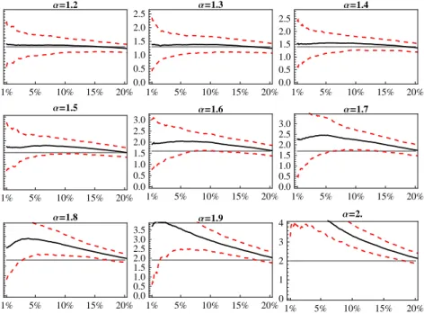
3.3.1. Hill estimation fork >1%. We begin the simulations with a time series length of 103, which is a usual sample length for real-world financial data, i.e., it equates to
approximately 4 years of daily returns of a stock. Figure1shows the 95% confidence intervals3 of the Hill estimate for different α for all k. It can be seen that it is very difficult to statistically distinguish between different tail exponents α and it is very unclear which optimal k we should choose.
Figure2 shows much more precise results for a time series of length 106. This allows
for narrow confidence intervals, but even with this exact result we can see that the Hill estimator is problematic as it overestimates the value of the tail exponent and we cannot pick the optimalk even from this large grid of simulated data. The only way of estimating the tail exponent would be to pickk, estimate the tail exponent, and compare it to the grid of simulated confidence intervals. But we would still need at least a 106 sample size to achieve an exact result. As we can see in Figure1, we cannot get a statistically significant estimate on data with length 103. Table1shows
the optimal value of k, where the Hill estimator gives a good estimate of the tail exponentα4. α n 1.1 1.2 1.3 1.4 1.5 1.6 1.7 1.8 1.9 2 103 9.11% 15.92% 17.28% 18.53% 20.42% 20.84% 21.15% 21.78% 22.20% 21.88% 104 8.88% 13.55% 17.17% 18.73% 19.95% 20.83% 21.38% 21.71% 21.97% 22.01% 105 8.04% 13.73% 16.84% 18.78% 20.04% 20.80% 21.35% 21.73% 21.98% 22.10% 106 8.29% 13.60% 16.80% 18.74% 20.00% 20.80% 21.35% 21.73% 21.98% 22.15%
Table 1. Optimal k for various sample lengths n from 103 to 106
The figures suggest that the Hill estimator does not overestimate the tail exponent on the 1% tail so strongly. Thus, we repeat the exercise for k ≤1%.
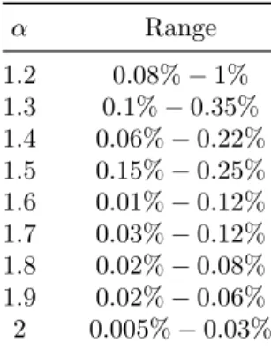
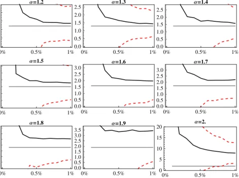
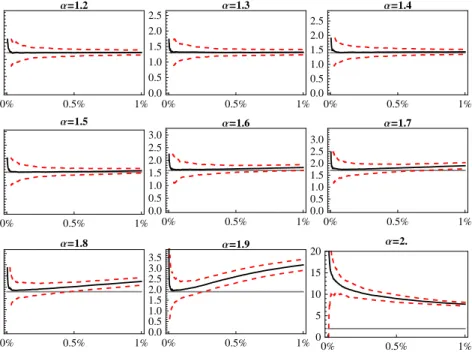
3.3.2. Hill estimation for k ≤ 1%. Figures 3, 4, 5, and 6 show the behavior of the Hill estimator on generated datasets with length 103 up to 106. The results suggest
that it makes no sense to use the Hill estimator for tail exponent estimation even on the 105 dataset. For example, α of 1.2,1.3,1.4,1.5, and 1.6 cannot be statistically
distinguished from each other. Only the dataset with length 106shows better results.
Using the simulations on such a long dataset, we can choose the optimal range of
k. More exactly, the optimal k interval is such where the estimated value of the tail exponent does not deviate from its theoretical value by more than 5%. Table 2
shows the optimal sets ofk where the Hill estimator was a good estimate of the tail exponent. α Range 1.2 0.08%−1% 1.3 0.1%−0.35% 1.4 0.06%−0.22% 1.5 0.15%−0.25% 1.6 0.01%−0.12% 1.7 0.03%−0.12% 1.8 0.02%−0.08% 1.9 0.02%−0.06% 2 0.005%−0.03%
Table 2. Optimal range of k for series length 106 fork ≤1%
1% 5% 10% 15% 20% 0.0 0.5 1.0 1.5 2.0 Α=1.2 1% 5% 10% 15% 20% 0.0 0.5 1.0 1.5 2.0 2.5 Α=1.3 1% 5% 10% 15% 20% 0.0 0.5 1.0 1.5 2.0 2.5 Α=1.4 1% 5% 10% 15% 20% 0.0 0.5 1.0 1.5 2.0 2.5 3.0 Α=1.5 1% 5% 10% 15% 20% 0.0 0.5 1.0 1.5 2.0 2.5 3.0 Α=1.6 1% 5% 10% 15% 20% 0.0 0.5 1.0 1.5 2.0 2.5 3.0 Α=1.7 1% 5% 10% 15% 20% 0.0 0.5 1.0 1.5 2.0 2.5 3.0 3.5 Α=1.8 1% 5% 10% 15% 20% 0.0 0.5 1.0 1.5 2.0 2.5 3.0 3.5 Α=1.9 1% 5% 10% 15% 20% 0 1 2 3 4 Α=2.
Figure 1. Hill estimate of the tail exponent on the 1%–20% tail, 103 length
1% 5% 10% 15% 20% 0.0 0.5 1.0 1.5 2.0 Α=1.2 1% 5% 10% 15% 20% 0.0 0.5 1.0 1.5 2.0 2.5 Α=1.3 1% 5% 10% 15% 20% 0.0 0.5 1.0 1.5 2.0 2.5 Α=1.4 1% 5% 10% 15% 20% 0.0 0.5 1.0 1.5 2.0 2.5 3.0 Α=1.5 1% 5% 10% 15% 20% 0.0 0.5 1.0 1.5 2.0 2.5 3.0 Α=1.6 1% 5% 10% 15% 20% 0.0 0.5 1.0 1.5 2.0 2.5 3.0 Α=1.7 1% 5% 10% 15% 20% 0.0 0.5 1.0 1.5 2.0 2.5 3.0 3.5 Α=1.8 1% 5% 10% 15% 20% 0.0 0.5 1.0 1.5 2.0 2.5 3.0 3.5 Α=1.9 1% 5% 10% 15% 20% 0 1 2 3 4 Α=2.
0% 0.5% 1% 0.0 0.5 1.0 1.5 2.0 Α=1.2 0% 0.5% 1% 0.0 0.5 1.0 1.5 2.0 2.5 Α=1.3 0% 0.5% 1% 0.0 0.5 1.0 1.5 2.0 2.5 Α=1.4 0% 0.5% 1% 0.0 0.5 1.0 1.5 2.0 2.5 3.0 Α=1.5 0% 0.5% 1% 0.0 0.5 1.0 1.5 2.0 2.5 3.0 Α=1.6 0% 0.5% 1% 0.0 0.5 1.0 1.5 2.0 2.5 3.0 Α=1.7 0% 0.5% 1% 0.0 0.5 1.0 1.5 2.0 2.5 3.0 3.5 Α=1.8 0% 0.5% 1% 0.0 0.5 1.0 1.5 2.0 2.5 3.0 3.5 Α=1.9 0% 0.5% 1% 0 5 10 15 20 Α=2.
Figure 3. Hill estimate of the tail exponent on the ≤1% tail, 103 length
0% 0.5% 1% 0.0 0.5 1.0 1.5 2.0 Α=1.2 0% 0.5% 1% 0.0 0.5 1.0 1.5 2.0 2.5 Α=1.3 0% 0.5% 1% 0.0 0.5 1.0 1.5 2.0 2.5 Α=1.4 0% 0.5% 1% 0.0 0.5 1.0 1.5 2.0 2.5 3.0 Α=1.5 0% 0.5% 1% 0.0 0.5 1.0 1.5 2.0 2.5 3.0 Α=1.6 0% 0.5% 1% 0.0 0.5 1.0 1.5 2.0 2.5 3.0 Α=1.7 0% 0.5% 1% 0.0 0.5 1.0 1.5 2.0 2.5 3.0 3.5 Α=1.8 0% 0.5% 1% 0.0 0.5 1.0 1.5 2.0 2.5 3.0 3.5 Α=1.9 0% 0.5% 1% 0 5 10 15 20 Α=2.
0% 0.5% 1% 0.0 0.5 1.0 1.5 2.0 Α=1.2 0% 0.5% 1% 0.0 0.5 1.0 1.5 2.0 2.5 Α=1.3 0% 0.5% 1% 0.0 0.5 1.0 1.5 2.0 2.5 Α=1.4 0% 0.5% 1% 0.0 0.5 1.0 1.5 2.0 2.5 3.0 Α=1.5 0% 0.5% 1% 0.0 0.5 1.0 1.5 2.0 2.5 3.0 Α=1.6 0% 0.5% 1% 0.0 0.5 1.0 1.5 2.0 2.5 3.0 Α=1.7 0% 0.5% 1% 0.0 0.5 1.0 1.5 2.0 2.5 3.0 3.5 Α=1.8 0% 0.5% 1% 0.0 0.5 1.0 1.5 2.0 2.5 3.0 3.5 Α=1.9 0% 0.5% 1% 0 5 10 15 20 Α=2.
Figure 5. Hill estimate of the tail exponent on the ≤1% tail, 105 length
0% 0.5% 1% 0.0 0.5 1.0 1.5 2.0 Α=1.2 0% 0.5% 1% 0.0 0.5 1.0 1.5 2.0 2.5 Α=1.3 0% 0.5% 1% 0.0 0.5 1.0 1.5 2.0 2.5 Α=1.4 0% 0.5% 1% 0.0 0.5 1.0 1.5 2.0 2.5 3.0 Α=1.5 0% 0.5% 1% 0.0 0.5 1.0 1.5 2.0 2.5 3.0 Α=1.6 0% 0.5% 1% 0.0 0.5 1.0 1.5 2.0 2.5 3.0 Α=1.7 0% 0.5% 1% 0.0 0.5 1.0 1.5 2.0 2.5 3.0 3.5 Α=1.8 0% 0.5% 1% 0.0 0.5 1.0 1.5 2.0 2.5 3.0 3.5 Α=1.9 0% 0.5% 1% 0 5 10 15 20 Α=2.
In order to estimate the true tail exponent, we need a dataset with length of at least 106, otherwise inference of the tail exponent may be strongly misleading and
rejection of the L´evy stable regime not appropriate. For the sake of clarity we have to note that the results for theα = 2 should be interpreted with caution as it is the special case of Gaussian distribution which does not have heavy tails. Thus the Hill estimator is not appropriate in this case.
In the next section, we develop a Monte Carlo-based tail exponent estimator which deals with all of these problems.
4. Tail exponent estimator based on Monte Carlo simulations
After our broad study of the theoretical properties of the Hill estimator, we utilize the results and introduce a Monte Carlo-based estimator. The Monte Carlo technique provides an attractive method of building exact tests from statistics whose finite sample distribution is intractable but can be simulated.
We construct our Monte Carlo-based tail exponent estimator as follows.
(1) Generate 1,000 i.i.d. α−stable distributed random variables Xα0 of length
n, i.e. xα0
1 , x
α0
2 , . . . , xαn0 ∼ S(α0,0,
√
2/2,0), for each α0 parameter from the
range [1.01,2] with step 0.01.
(2) For each Xα0, estimate the tail exponent using the Hill estimator for all k from the interval (1%−20%), i.e. ˆαα0,k.
(3) From Monte Carlo simulations compute the expected value E[ ˆαα0,k] of the Hill estimator for all k and allα0.
(4) Using the Hill estimator estimate the tail exponent ˆαemp,k on an empirical
dataset of length n for all k from the interval (1%−20%). (5) Our Monte Carlo-based estimator ˆαM C is defined as:
(11) αˆM C = arg min
α0∈[1.01,2]
X
k
|αˆemp,k−E[ ˆαα0,k]|
In other words, we simulate random variables X of length n for 100 different α’s (representing the tail parameter) 1,000 times.5 On these random variables we esti-mate the tail exponent using the Hill estimator on the (1%−20%) tail (as we have shown in the previous section, the Hill estimator does not really work onk ≤1% for
1 1.2 1.4 1.6 1.8 2 1.0 1.2 1.4 1.6 1.8 2.0 1.0 1.2 1.4 1.6 1.8 2.0 Α Α ` H
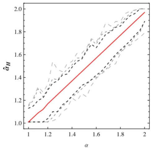
Figure 7. Plots of 99%, 95%, and 90% quantiles of our Monte Carlo-based tail exponent estimator Carlo-based on 100 simulations.
series of lengths ≤106). Using the simulated variables we get the expected value of
the Hill estimator for all k and allα0.
After we have obtained the behavior of the Hill estimator for a large grid of different tail exponents and k, we can estimate the tail exponent on the empirical dataset. First, we estimate the tail exponent using the Hill estimator for all values of k. As the last step, we minimize the loss function which is defined by Equation11through the whole simulated grid of α0. Our Monte Carlo-based tail exponent estimate ˆαM C
is the value for which the distance betweenE[ ˆαα0,k] and ˆαemp,k is minimal (Equation
11).
4.1. Properties of αˆM C. In this section we would like to study the finite sample
properties of our estimation method. For this purpose, we will again use the Monte Carlo procedure, which will help us to test the estimator. We simulate independent identically α−stable distributed random variables of length n from S(α,0,√2/2,0) with varying α ∈ [1.01,2] with step 0.01. For each simulated sample, we apply our method and estimate the tail exponent. This Monte Carlo simulation allows us to derive the finite sample properties of our estimator, so we can get the confidence interval of the estimates.
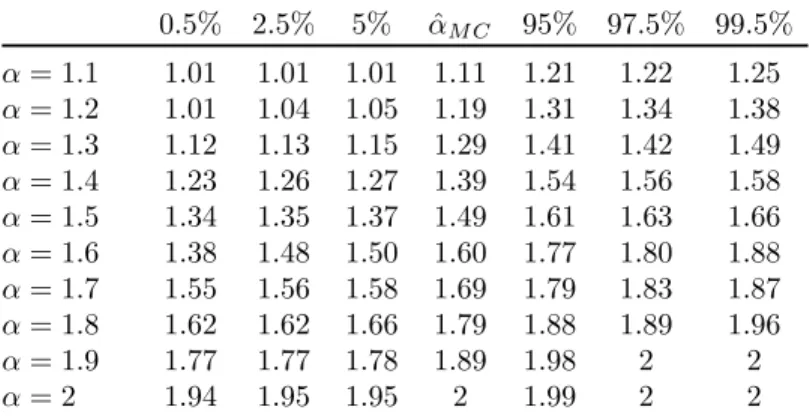
Figure7plots the 99%, 95%, and 90% quantiles of our tail exponent estimator based on 100 simulations. Table3provides exact simulated confidence intervals for several values of α.
0.5% 2.5% 5% αˆM C 95% 97.5% 99.5% α= 1.1 1.01 1.01 1.01 1.11 1.21 1.22 1.25 α= 1.2 1.01 1.04 1.05 1.19 1.31 1.34 1.38 α= 1.3 1.12 1.13 1.15 1.29 1.41 1.42 1.49 α= 1.4 1.23 1.26 1.27 1.39 1.54 1.56 1.58 α= 1.5 1.34 1.35 1.37 1.49 1.61 1.63 1.66 α= 1.6 1.38 1.48 1.50 1.60 1.77 1.80 1.88 α= 1.7 1.55 1.56 1.58 1.69 1.79 1.83 1.87 α= 1.8 1.62 1.62 1.66 1.79 1.88 1.89 1.96 α= 1.9 1.77 1.77 1.78 1.89 1.98 2 2 α= 2 1.94 1.95 1.95 2 1.99 2 2
Table 3. Quantiles of our estimation method.
In comparison with the Hill estimator, or any other tail exponent estimator, our method has several advantages. The largest advantage is that the method is not sensitive to the choice of k, unlike most of the other estimation methods discussed in the previous text. Our method also works well for smaller samples, i.e. 103, as it
yields much narrower confidence intervals compared to the Hill estimator.
5. Empirical study
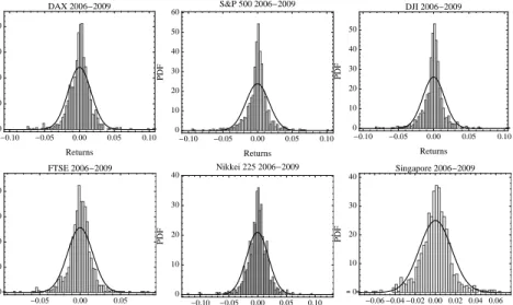
To illustrate the power of our tail exponent estimation method, we employ empirical data. We use the daily returns of the following stock market indices: the German DAX 30, the U.S. S&P 500 and Dow Jones Industrial 30 (DJI), the London FTSE 100, the Nikkei 225, and the Singapore Straits Times from the beginning of 2002 to the end of 2009. More precisely, we choose the last 2,000 observations for each index and divide them into two equal periods, 2002–2005 and 2006–2009, each containing 1,000 observations. This way, we can compare different world stock market indices and their behavior before and during the current financial crisis .
Figures 9 and 10 show the histograms of the tested indices. Figure 9 shows the histograms for the first period 2002–2005, while Figure 10shows the histograms for the second period 2006–2009. All the data are leptokurtic, showing excessive peaks around the mean and thicker tails than those of the normal density. Moreover, the data from the second period tend to show even more excessive kurtosis and heavier tails than the ones from the first period. This is probably caused by the large price movements that occurred during the deep financial turmoil in the years 2007– 2009. By contrast, the first period of stable growth is closer to the standard normal distribution.
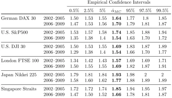
We use our Monte Carlo method to estimate the tail exponents for all the datasets. Before we start the estimations, we set the lengthn of the simulated series from our algorithm to 1,000 so that it corresponds to the length of the empirical dataset and we can statistically compare the estimates. Table4shows the tail exponent estimates with confidence intervals. Let us further demonstrate the estimation method on the
Empirical Confidence Intervals
0.5% 2.5% 5% αˆM C 95% 97.5% 99.5% German DAX 30 2002–2005 1.50 1.53 1.55 1.64 1.77 1.8 1.85 2006–2009 1.47 1.53 1.56 1.70 1.79 1.81 1.87 U.S. S&P500 2002–2005 1.53 1.57 1.58 1.74 1.85 1.88 1.94 2006–2009 1.35 1.38 1.4 1.54 1.63 1.70 1.72 U.S. DJI 30 2002–2005 1.50 1.53 1.55 1.69 1.83 1.87 1.89 2006–2009 1.29 1.38 1.4 1.54 1.66 1.70 1.77 London FTSE 100 2002–2005 1.34 1.42 1.43 1.57 1.69 1.69 1.71 2006–2009 1.50 1.55 1.55 1.69 1.82 1.87 1.91 Japan Nikkei 225 2002–2005 1.79 1.81 1.84 1.93 1.98 2 2 2006–2009 1.58 1.60 1.62 1.77 1.88 1.89 1.89 Singapore Straits 2002–2005 1.72 1.72 1.74 1.85 1.94 1.95 1.97 2006–2009 1.47 1.50 1.52 1.66 1.78 1.81 1.87
Table 4. Exact confidence intervals (quantiles) of the estimated tail exponent α. 1% 5% 10% 15% 20% 1 2 3 4 Α=1.55 1% 5% 10% 15% 20% 1 2 3 4 5 Α=1.69 1% 5% 10% 15% 20% 1 2 3 4 5 Α=1.87
Figure 8. Plot of Hill estimates through different k for the FTSE index (second period of 2006–2009) for α = 1.55, α = 1.69, and α = 1.87, which are our ˆαM C with the 0.025% and 97.5% quantiles.
example of the London FTSE 100 index for the second period. Figure 8 plots the empirical Hill estimates through differentk and compares them to 1,000 simulations of α = 1.55, α = 1.69, and α = 1.87 (these are our Monte Carlo estimates with the 0.025% and 97.5% quantiles). It is immediately visible from the plots that the
loss function defined in our estimation algorithm reaches its minimum forα = 1.69. We plot another two cases just for illustration of what our estimate looks like at the critical levels. After minimizing the loss function and choosing the tail exponent, we derive the finite sample properties of the estimate. From Table 4, we can see that 1.55 and 1.87 are the 0.025% and 97.5% quantiles.
Unlike the classical Hill estimation procedure, we can see that our method is not sensitive to the choice of k. Moreover, it is a much stronger result for the tail exponent, as it accounts for all possible k’s, not only the one chosen. Using the classical Hill estimation procedure, we would selectkand compute the tail exponent, but as we discussed in the previous text, there is always a trade-off between bias and variance when choosing the optimal k. Our method reduces this problem. Finally, the sample on which we estimate the tail exponent is quite small. In previous sections we showed that Hill estimation does not work well for such small samples, but our method works fine.
6. Conclusion
In this paper, we have researched the finite sample behavior of the Hill estimator under α−stable distributions and we introduce a Monte Carlo-based method of es-timation for the tail exponent.
First of all, we provide Monte Carlo confidence intervals for the Hill estimator under differentα’s and k on the intervalk ∈(0,20%] of sample size 103 up to 106. We also
provide the optimal range ofk for the series length 106. Based on our simulations, we
conclude that in order to estimate the true tail exponent using the Hill estimator, we need a dataset of at least 106 length, i.e., high frequency data, otherwise inference of
the tail exponent may be strongly misleading and rejection of the L´evy stable regime not appropriate.
In the second part of the paper, we utilize the results and introduce a tail exponent procedure based on Monte Carlo simulations. It is based on the idea of simulating a large grid of random variables from the L´evy stable distribution with different α
exponents and estimating the tail exponent using the Hill estimator for all different
k. After obtaining the behavior of the Hill estimator on this large grid of different tail exponents andk, all we need to do is to estimate the tail exponent on the empirical dataset for all k’s and compare all the values with the simulated grid. Using this algorithm we get estimates of the tail exponent.
In comparison with the Hill estimator, or any other tail exponent estimator, our method has several advantages. The largest advantage is that it is not sensitive
to the choice of k. Moreover, the method works well for small samples. The new estimator gives unbiased results with symmetrical confidence intervals.
Finally, we illustrate the power of our tail exponent estimation method on an empir-ical dataset. We use daily returns of leading world stock markets: the German DAX, the U.S. S&P 500 and Dow Jones Industrial (DJI), the London FTSE, the Nikkei 225, and the Singapore Straits Times from the beginning of 2002 to the end of 2009. We divide this period into two equal sub-periods and compare the tail exponents estimated using our method.
References
Bouchaud, J. P. and M. Potters (2001). Theory of Financial Risks: From Statistical Physics to Risk Management. Cambridge: Cambridge University Press.
Buchanan, M. (2002). The physics on the trading floor. Nature 10-12(415).
Dacorogna, M., R. Gen¸cay, U. Mueller, and O. Pictet (2001). An Introduction to High-Frequency finance. Academic press.
Dekkers, A. L. M., J. H. J. Einmahl, and L. De Haan (1989). A moment estimator for the index of an extreme-value distribution. The Annals of Statistics 17(4), 1833–1855.
Embrechts, P., C. Kluppelberg, and T. Mikosch (1997). Modelling Extremal Events for Insurance and Finance. Heidelberg: Springer Verlag.
Fama, E. (1965). The behavior of stock prices. Journal of Business (38), 34–105. Goldie, C. M. and R. L. Smith (1987). Slow variation with remainder: Theory and
applications. Quarterly Journal of Mathematics, Oxford 2nd Series 38(1), 45–71. Hall, P. (1990). Using the bootstrap to estimate mean squared error and select smoothing parameters in nonparametric probles. Journal of Multivariate Analy-sis 32(2), 177–203.
Hill, B. M. (1975). A simple general approach to inference about the tail of a distribution. The Annals of Statistics 3(5), 1163–1174.
Hsing, T. (1991). On tail index estimation using dependent data. Annals of Statis-tics 19(3), 1547–1569.
Lux, T. (1996). The stable paretian hypothesis and the frequency of large returns.
Applied Financial Economics 6, 463–475.
Mandelbrot, B. (1963). The variation of certain speculative prices. Journal of Busi-ness (26), 394–419.
Mantegna, R., Z. Palagyi, and H. Stanley (1999). Applications of statistical mechan-ics to finance. Physica A 274(1-2), 216–221.
Mantegna, R. and H. Stanley (2000). An Introduction to Econophysics. Cambridge: Cambridge University Press.
Mason, D. M. (1982). Laws of large numbers for sums of extreme values. Annals of Probability 10(3), 754–764.
McCulloch, J. H. (1996). Financial applications of stable distributions (Handbook of Statistics ed.), Volume 14. Elsevier.
Mittnik, S., P. M. S., and S. T. Rachev (1998). A tail estimator for the index of the stable paretian distribution. Communications in statistics. Theory and methods 27(5), 1239–1262.
Nolan, J. P. (2003). Stable Distributions: Models for Heavy Tailed Data. Boston, MA: Birkhauser.
Pickands, J. (1975). Statistical inference using extreme order statistics. Annals of Statistics 3(1), 119–131.
Plerou, V., P. Gopikrishnan, B. Rosenow, L. A. N. Amaral, and H. E. Stanley (2000). A random matrix theory approach to financial cross-corelations. Physica A 287 (3-4), 374–382.
Rachev, S. T. and S. Mittnik (2000). Stable Paretian Models in Finance. New York: Wiley.
Resnick, S. I. (2007). Heavy Tail Phenomena: Probabilistic and Statistical Model-ing. Springer Series in Operations Research and Financial Engineering. New York: Springer.
Samorodnitsky, G. and M. S. Taqqu (1994).Stable Non-Gaussian Random Processes. New York: Chapman and Hall.
Stanley, H. (2003). Statistical physics and economic fluctuations: do outliers exist?
Physica A 318(1-2), 279–292.
Stanley, H., L. Amaral, P. Gopikrishnan, and V. Plerou (2000). Scale invariance and universality of economic fluctuations. Physica A 283(1-2), 31–41.
Voit, J. (2005). The Statistical Mechanics of Financial Markets. Heidelberg: Springer-Verlag Berlin.
Wagner, N. and T. A. Marsh (2004). Tail index estimation in small smaples sim-ulation results for independent and arch-type financial return models. Statistical Papers 45(4), 545–561.
Weron, R. (2001). L´evy-stable distributions revisited: Tail index > 2 does not exclude the levy-stable regime. International Journal of Modern Physics C 12, 209–223.
Zolotarev, V. M. (1986). One-Dimensional Stable Distributions, Volume 65 of Amer. Math. Soc. Transl. of Math. Monographs. Providence, RI: Amer. Math. Soc.
Appendix -0.06-0.04-0.02 0.00 0.02 0.04 0.06 0 10 20 30 40 Returns PDF DAX 2002-2005 -0.04 -0.02 0.00 0.02 0.04 0 10 20 30 40 50 60 Returns PDF S&P 500 2002-2005 -0.06-0.04-0.02 0.00 0.02 0.04 0.06 0 10 20 30 40 50 60 Returns PDF DJI 2002-2005 -0.04-0.02 0.00 0.02 0.04 0 10 20 30 40 50 Returns PDF FTSE 2002-2005 -0.04 -0.02 0.00 0.02 0.04 0 10 20 30 40 Returns PDF Nikkei 225 2002-2005 -0.04 -0.02 0.00 0.02 0.04 0 10 20 30 40 50 Returns PDF Singapore 2002-2005
Figure 9. Histograms of all indices for the first period compared with the standard normal distribution
-0.10 -0.05 0.00 0.05 0.10 0 10 20 30 40 Returns PDF DAX 2006-2009 -0.10 -0.05 0.00 0.05 0.10 0 10 20 30 40 50 60 Returns PDF S&P 500 2006-2009 -0.10 -0.05 0.00 0.05 0.10 0 10 20 30 40 50 Returns PDF DJI 2006-2009 -0.05 0.00 0.05 0 10 20 30 40 Returns PDF FTSE 2006-2009 -0.10 -0.05 0.00 0.05 0.10 0 10 20 30 40 Returns PDF Nikkei 225 2006-2009 -0.06-0.04-0.02 0.00 0.02 0.04 0.06 0 10 20 30 40 Returns PDF Singapore 2006-2009
Figure 10. Histograms of all indices for the second period compared with the standard normal distribution
IES Working Paper Series
2009
1.František Turnovec : Fairness and Squareness: Fair Decision Making Rules in the EU Council?
2.Radovan Chalupka : Improving Risk Adjustment in the Czech Republic
3.Jan Průša : The Most Efficient Czech SME Sectors:An Application of Robust Data Envelopment Analysis
4.Kamila Fialová, Martina Mysíková : Labor Market Participation: The Impact of Social Benefits in the Czech Republic
5.Kateřina Pavloková : Time to death and health expenditure of the Czech health care system
6.Kamila Fialová, Martina Mysíková : Minimum Wage: Labour Market Consequences in the Czech Republic
7.Tomáš Havránek : Subsidy Competition for FDI: Fierce or Weak?
8.Ondřej Schneider : Reforming Pensions in Europe: Economic Fundamentals and Political Factors
9.Jiří Witzany : Loss, Default, and Loss Given Default Modeling
10. Michal Bauer, Julie Chytilová : Do children make women more patient? Experimental evidence from Indian villages
11. Roman Horváth : Interest Margins Determinants of Czech Banks
12. Lenka Šťastná : Spatial Interdependence of Local Public Expenditures: Selected Evidence from the Czech Republic
13.František Turnovec : Efficiency of Fairness in Voting Systems
14. Martin Gregor, Dalibor Roháč : The Optimal State Aid Control: No Control
15. Ondřej Glazar, Wadim Strielkowski : Turkey and the European Union: possible incidence of the EU accession on migration flows
16.Michaela Vlasáková Baruníková : Option Pricing: The empirical tests of the Black-Scholes pricing formula and the feed-forward networks
17.Eva Ryšavá, Elisa Galeotti : Determinants of FDI in Czech Manufacturing Industries between 2000-2006
18. Martin Gregor, Lenka Šťastná : Mobile criminals, immobile crime: the efficiency of decentralized crime deterrence
19. František Turnovec : How much of Federalism in the European Union
20. Tomáš Havránek : Rose Effect and the Euro: The Magic is Gone
21. Jiří Witzany : Estimating LGD Correlation
22. Linnéa Lundberg, Jiri Novak, Maria Vikman : Ethical vs. Non-Ethical – Is There a Difference? Analyzing Performance of Ethical and Non-Ethical Investment Funds
23. Jozef Barunik, Lukas Vacha : Wavelet Analysis of Central European Stock Market Behaviour During the Crisis
24. Michaela Krčílková, Jan Zápal : OCA cubed: Mundell in 3D
25. Jan Průša : A General Framework to Evaluate Economic Efficiency with an Application to British SME
26. Ladislav Kristoufek : Classical and modified rescaled range analysis: Sampling properties under heavy tails
29. Jiri Novak, Dalibor Petr : Empirical Risk Factors in Realized Stock Returns
30. Karel Janda, Eva Michalíková, Věra Potácelová : Vyplácí se podporovat exportní úvěry?
31. Karel Janda, Jakub Mikolášek, Martin Netuka : The Estimation of Complete Almost Ideal Demand System from Czech Household Budget Survey Data
32. Karel Janda, Barbora Svárovská : Investing into Microfinance Investment Funds
2010
1. Petra Benešová, Petr Teplý : Main Flaws of The Collateralized Debt Obligation’s Valuation Before And During The 2008/2009 Global Turmoil
2. Jiří Witzany, Michal Rychnovský, Pavel Charamza : Survival Analysis in LGD Modeling
3. Ladislav Kristoufek : Long-range dependence in returns and volatility of Central European Stock Indices
4. Jozef Barunik, Lukas Vacha, Miloslav Vosvrda : Tail Behavior of the Central European Stock Markets during the Financial Crisis
5. Onřej Lopušník : Různá pojetí endogenity peněz v postkeynesovské ekonomii: Reinterpretace do obecnější teorie
6. Jozef Barunik, Lukas Vacha : Monte Carlo-Based Tail Exponent Estimator
All papers can be downloaded at: http://ies.fsv.cuni.cz
Univerzita Karlova v Praze, Fakulta sociálních věd Institut ekonomických studií [UK FSV – IES] Praha 1, Opletalova 26