Distributed and Robust Support Vector Machine

(1)

Yangwei Liu

1

_{, Hu Ding}

2

_{, Ziyun Huang}

3

_{, and Jinhui Xu}

4

1 Department of Computer Science and Engineering, State University of New York at Buffalo, US

2 Department of Computer Science and Engineering, Michigan State University, US

Abstract

In this paper, we consider the distributed version of Support Vector Machine (SVM) under the coordinator model, where all input data (i.e., points in _Rd _{space) of SVM are arbitrarily}

distributed amongk nodes in some network with a coordinator which can communicate with all nodes. We investigate two variants of this problem, with and without outliers. For distributed SVM without outliers, we prove a lower bound on the communication complexity and give a distributed (1−)-approximation algorithm to reach this lower bound, whereis a user specified small constant. For distributed SVM with outliers, we present a (1−)-approximation algorithm to explicitly remove the influence of outliers. Our algorithm is based on a deterministic distributed toptselection algorithm with communication complexity ofO(klog (t)) in the coordinator model. Experimental results on benchmark datasets confirm the theoretical guarantees of our algorithms.

1998 ACM Subject Classification F.2.2 Nonnumerical Algorithms and Problems

Keywords and phrases Distributed Algorithm, Communication Complexity, Robust Algorithm, SVM

Digital Object Identifier 10.4230/LIPIcs.ISAAC.2016.54

1 Introduction

Training a Support Vector Machine (SVM) [5] in a distributed setting is a commonly encountered problem in the big data era. This could be due to the fact that the data set is too large to be stored in a centralized site (e.g.,bioinformatics data [15]), or simply because the data set is collected in a distributed environment (e.g.,wireless sensor network data [22]). In many scenarios, large volume data transmission between different sites could be rather expensive and time consuming. In some applications, this may not even be allowed due to privacy concerns. Thus efficient distributed SVM algorithms are needed to minimize the communication cost and meanwhile preserve the quality of solution.

In recent years, a significant amount of effort has been devoted to this problem ([9, 3, 12, 14, 4, 16, 8, 18, 6]), and a number of distributed SVM algorithms with different strength have been developed. However most of them are still suffering from various limitations, such as high communication complexity, sub-optimal quality of solution, and slow convergence

∗ _{The research of this work was supported in part by NSF through grants CCF-1422324, IIS-1422591,}

and CNS-1547167. Ding was supported by a start-up fund from Michigan State University.

(2)

rate. For instance, one type of extensively studied algorithms in recent years are the family ofincremental constructionalgorithms [9, 3].

Such algorithms often have good performance in practice and some other nice features related to robustness and decentralization; but they generally do not have theoretical guarantee on the communication complexity, and some of them even have no quality guarantee on their solutions. Another type of popular algorithms are those which parallelize existing centralized algorithms ([12, 14, 4]). These algorithms typically focus on enhancing the ability of dealing with extremely large size data sets, but in general have no quality guarantee on communication complexity. There are also another family of algorithms called distributed stochastic gradient descent algorithms [20]; the main issue of such algorithms is that their running time (or number of iteration) is mostly sub-optimal, and they do not have a guarantee on communication cost. Very recently, there is an interesting result [2] which presents a similar lower bound on communication cost. However their lower bound applies only to those coreset-based algorithms, not the general algorithms, whereas the lower bound result in this paper is applicable to any distributed SVM algorithm.

From a geometric point of view, training an SVM can be interpreted as finding a hyperplane that separates two classes of points while maximizing the separating margin. It is also well known to be equivalent to computing the polytope distance of the two point sets. Recent research [10] shows that we can find an (1−)-approximation of the polytope distance using Gilbert algorithm with a running time linearly depending on the input size. Roughly speaking, Gilbert algorithm is a gradient descent procedure that in each step greedily computes an optimal direction along which the primal solution should improve.

In this paper we present a distributed SVM algorithm that is theoretically guaranteed to have the lowest possible communication cost together with a guaranteed near-optimal solution, based on the classical Gilbert algorithm [11]. Comparing to previous distributed SVM algorithms, our algorithm has several advantages. (1) Our algorithm has a communication complexity which is theoretically guaranteed to reach the lower bound; (2) it does not make any assumption on the input data and its distribution; (3) its running time is only linearly dependent on the input size; and (4) it produces a (1−)-approximation for the problem which is sparse (i.e.,the number of support vectors is small).

Since SVM is well known to be sensitive to outliers, we also consider the case of distributed SVM with outliers. We show that it is possible to explicitly avoid the influence of outliers in distributed settings by using a combinatorial tool called Random Gradient Descent (RGD)tree [7] to achieve a (1−)-approximation on the quality of solution and meanwhile significantly reduce the communication cost. An underlying technique used for reducing the communication cost is an algorithm for the distributed selection problem (i.e., finding the

t-th smallest number from a set of numbers distributed inksites). This problem has been extensively studied in the past ([17, 21, 13]). The best result (in terms of communication cost) is a randomized algorithm [13] which has a communication complexity ofO(klog (t)). The best deterministic algorithm has a communication complexity ofO(klog2(t)). In this paper we give a deterministic algorithm with communication complexityO(klog (t)) in the coordinator model.

In this paper We will concentrate on one-class SVM first since it captures the main difficulty of the problem, and then extend the results to two-class SVM (in the full version of this paper). We also performed experiments on benchmark datasets to evaluate the performance of the algorithms (in the full version of the paper).

(3)

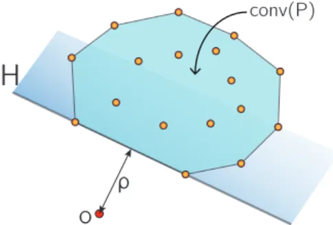
conv(P)

H

o

ρ

Figure 1One-class SVM is equivalent to

the polytope distance problem. ρis the poly-tope distance,His the separating hyperplane, with distance tooexactlyρ.

x

i

x

i+1

p

_i

o

Figure 2 One step of the Gilbert

Al-gorithm, updatingxitoxi+1.

2 Preliminaries

2.1 Equivalence between SVM and Polytope Distance

In this section, we give several definitions which will be used throughout the paper.

IDefinition 1. (One-class SVM): Given a point setP ⊆Rd, find a hyperplaneH separating

the origino andP such that the separating margin (i.e., the distance betweeno andH) is maximized.

It is well known that this problem is equivalent to the following problem of computing the polytope distance:

I Definition 2. (Polytope distance): Given a point set P ⊆ Rd, compute the shortest

distance between the originoand a pointpin the polytopeconv(P) (i.e.,the convex hull of

P).

I Lemma 3 ([10]). Given a point x which realizes the polytope distance of P ⊆ Rd, the hyperplaneH passing xand orthogonal tooxis the maximum separating hyperplane ofP. In other words, the polytope distance problem is equivalent to the one-class SVM problem.

Figure 1 provides an intuitive explanation of the equivalence between one-class SVM and polytope distance. Notice that the polytope distance problem can be formulated as a standard convex quadratic optimization problem, thus can be solved optimally using standard techniques inO(n3) time. However this approach is mostly impractical because of the high time complexity. Actually in many applications, a near-optimal approximate solution is sufficient. Thus it is desirable to design efficient approximation algorithms. A (1−)-approximation of the polytope distance can be defined as follows.

I Definition 4. ((1−)-approximation of polytope distance): x ∈ conv(P) achieves a (1−)-approximation of the polytope distance problem, if

kxk −p|x≤kxk,∀p∈P

wherep|x:=

hp,xi

kxk is the signed length of the projection ofponto vectorox.

In the rest of this paper, we also call the pointx, rather its distance too, as the approximation. This is only for ease of discussion, and does not affect the solution at all (since we can get the actual distance by simply computing the distance betweenxand o).

(4)

2.2 Gilbert Algorithm

Gilbert algorithm can be used to find a (1−)-approximation of the polytope distance problem. Roughly speaking, Gilbert algorithm starts with an initial solutionx1 being the closest point ofP to the origin. In stepi, the algorithm finds the pointpi∈P that has the

smallest projection distance to vectoroxi, and picks the point on the line segment [pi, xi] that is closest to the origin asxi+1. Figure 2 illustrates one step of Gilbert algorithm. Algorithm 1Gilbert Algorithm

1: INPUT: Addimensional point setP, the origino.

2: OUTPUT: A (1−)-approximation of the polytope distance ofP too.

3: Initializeito be 1. Find the pointp1that is closest too, letx1=p1

4: In stepi, letpi+1 be the point that has the smallestp|xi, letxi+1 be the point that is closest tooon line segment [xi, pi+1].

5: Returnxi+1when it is a (1−)-approximation. Otherwise goto Line 4 withi=i+ 1. Despite its simplicity, it has been shown [10] that Gilbert algorithm can actually find such a (1−)-approximation inO(1) steps. Formally, we have the following theorem.

ITheorem 5([10]). Gilbert algorithm succeeds after at most O(1)steps.

Since each step of the algorithm involves only computing the projection of all points in

P to a specific direction, which can be done in linear time, Gilbert algorithm has a total running time linearly depending onn=|P|which is the number of input points.

Besides the fast running time, Gilbert Algorithm (and its variants) has also many other properties that make it a good SVM solver.

1. The algorithm works for arbitrary kernels. Since the algorithm only requires the compu-tation of projection distance, which can be obtained by scalar product, we only need one kernel evaluation at each time when a projection distance is computed. This also implies that our proposed algorithms can be trivially kernelized.

2. The result is sparse, or in other words, the number of support vectors is small. In the kernelized version, the solutionxi is a linear combination of input points, and we can easily observe thatxi involves at most one more point in each step, so the total number of support vectors isO(1).

3 Communication Complexity of Distributed SVM

In a distributed setting, the point setP is arbitrarily distributed amongknodes. Based on different modes of communication, there are different models to be considered. In this paper we mainly study the widely used coordinator model which contains an extra coordinator node, and all other nodes are only allowed to communicate with the coordinator. The algorithm itself can be easily modified for a more general communication model,e.g., network of general topology. Such generalization will at most induce an additionalO(D) (whereD is the diameter of the network) [1] increase on the communication complexity.

We are interested in determining the minimum amount of communication that is needed to find a (1−)-approximation of the polytope distance problem. We define the communication cost as the number of points needed to be transfered between nodes, where transferring one

d-dimensional point (together with an optional O(d) constants) takesO(1) communication. This way of defining the communication cost simplifies the proof of Theorem 6. Below is our lower bound result.

(5)

ITheorem 6. A (1−)-approximation of the distributed polytope distance problem requires

Ω(kd)communication for any <

√

17−4 16d .

We prove Theorem 6 by giving a reduction from the followingk-ORproblem.

IDefinition 7(k-OR). Givenkplayers with each holding ann-bit binary vector, find the bitwise OR of allkvectors.

An example of the k-OR problem can be like the following: Player 1 holds vector (1,0,0,1,0), Player 2 holds (0,0,0,1,1), and Player 3 holds (1,1,0,0,1). Then the output should be the vector (1,1,0,1,1), where each bit is just the OR of the same bit of all players’ vectors. For the communication complexity of this problem we have the following result.

ILemma 8([19]). k-OR problem requiresΩ(nk)communication in the coordinator model. Proof of Theorem 6. We prove Theorem 6 by reducing thek-OR problem to the problem of finding an-approximation of distributed polytope distance.

Given an instance of the k-OR problem with k players each holding an n-bit binary vector, construct an instance of distributed polytope distance ind=ndimensional space withknodes as follows:

For playeri, forj = 1,· · · , d, if thej’th bit of his vector is 0, add pointej to node i’s

point set; otherwise add pointλej to its point set, whereej = (0,· · ·,0 | {z } j-1 ,1,0,· · · ,0 | {z } d-j ) is the

d-dimensional point whose only non-zero entry is thej’th coordinate with value 1, andλis a constant smaller than 1 to be determined later.

In this construction, each node holds exactly dpoints, and there arekdpoints in total. Since for thej’th point there are only two possible positions to place it,i.e.,ej orλej, there will be points from different nodes sharing the same position. This does not affect the proof, since we can add a small enough perturbation to points sharing the same location.

IDefinition 9(Configuration). A configurationC of an instance of the polytope distance problem constructed as above is a size dpoint set, where the i’th point is λei if there is

at least oneλei in the point sets of all nodes; otherwise thei’th point is set to beei. The orderof a configurationC is the number ofλeit contains.

It is easy to see that a configuration encodes the solution of the correspondingk-OR problem. So if we can find out the configuration based on an-approximation solution of the distributed polytope distance problem, we can solve thek-OR problem, thus proving Theorem 6. The following lemma ensures that we can indeed achieve that.

ILemma 10. If <

√

17−4

16d , it is possible to determine the configuration purely based on an -approximation of the distributed polytope distance problem withλsatisfying 1₂−q1

4− d 1− < λ <min{p 1−d(1−(1−)2₎_,₍1 2+ q 1 4− d 1−)}. Notice that < √ 17−4 16d guarantees that 1 4 − d 1− >0, 1−d(1−(1−) 2₎ _>_{0, as well as} 1 2− q 1 4− d 1− < p

1−d(1−(1−)2_{). Thus such a}_λ_{always exists. Denote the polytope} distance of a configuration C as ρ(C), the order of C as order(C). We call the set of configurations with the same orderd0 as an order-d0 layer of configurations. We prove Lemma 10 in two steps:

Claim 1: order(Ci) = order(Cj) =⇒ ρ(Ci) = ρ(Cj); order(Ci) > order(Cj) =⇒

(6)

Claim 2: a solutionxcan’t be an-approximation for more than one configuration in the same layer.

Proof of Claim 1. Consider a configuration C={p1, p2,· · · , pd}with orderd0. This means that there ared−d0 _{points with their only non-zero coordinate as 1, and}_d0 _{points with their}

non-zero coordinate asλ. Suppose that the pointx=α1p1+α2p2+· · ·+αdpd onconv(C) is the closest point to the origin. We observe that fori∈[1, d], we have 0< αi<1. This

can be proved by contradiction as follows. First of all, sincexis onconv(C), we naturally have 0≤αi ≤1 andP

iαi= 1. Suppose that there exists anαl= 0. This means that the l’th coordinate ofxis 0, and thusxis on the simplex spanned byC− {pl}. Notice that in this case, we haveopl perpendicular to the simplex spanned byC− {pl}. Thus,_∠oxpl< π₂

and∠oplx < π₂, which means that the projection of oonto xpl is within the line segment xpl, resulting in a point closer too thanx, contradicting the fact thatxis the closest point too. Thenα <1 follows immediately.

The above observation guarantees that the closest point toois always withinconv(C), instead of on the boundary. Now let us computeρ(C).

We partition the points ofC into two subsets based on their non-zero coordinates. C1 contains points whose non-zero coordinates are 1, andCλcontains the rest. By the symmetry of the dimensions, we can safely assume that C1 contains the firstd−d0 points, and Cλ

contains the latterd0 points without loss of generality. Now leta= ₍_d₋_d0₎1_λ₊_d01

λ

, and consider the pointx= (λa·1,· · ·, λa·1

| {z } d−d0 ,a λ·λ,· · ·, a λ·λ | {z } d0

). It is clear that (1)xis within the boundary

ofconv(C), since (d−d0)λa+d0a_λ = 1; and (2) the projection distance of any point inConto

oxis _kλa_x_k. Thusoxis perpendicular to the subspace spanned byC. Combining the above two facts, we know thatxis the closest point tooonconv(C), andρ(C) =koxk=q 1

(d−d0₎₊d0

λ2 . Sinceρ(C) depends only on the order of the configuration, we have proved the first half of Claim 1.

Since each layer of configuration has the same polytope distance, we letρd0 denote the polytope distance for order-d0 layer. Now for the second half of Claim 1, let us consider two consecutive layers with orderd0 andd0+ 1. Then we have

ρd0₊₁ ρd0 = s d+ ( 1 λ2 −1)d0 d+ (_λ12 −1)(d0+ 1) ≤ r d−(1−λ2₎ d (1) < s d−(1−p 1−d(1−(1−)2₎2₎ d = 1− (2)

in which inequality (1) holds because of _λ12 −1 > 0. Using (2), we immediately have

ρ_d0₊_t

ρd0 <(1−)

t_<₁₋_{. Thus the second part of Claim 1 is proved.}

J Proof of Claim 2. In order to prove Claim 2, we first make another observation of the -approximationxof configurationC={p1,· · · , pd}of orderd0. Sincexis an-approximation, by definition it has to be onconv(C). So xtakes the form ofx=P_α

ipi, andPαi = 1.

Also by definition, we havepi|x>(1−)kxk. Together with the definition ofpi|x, we have αi≥ (1−)kxk2 _{, if}_pi₌_ei 1− λ2 kxk 2 _{, otherwise.}

(7)

Then we have forpi =ei, αi = 1−X j6=i αj ≤ 1−( X j6=i,pj=ej (1−)kxk2+ X j6=i,pj=λej (1−) λ2 kxk 2₎ = 1−((d−d0−1)(1−)kxk2₊_d01− λ2 kxk 2₎ = ( 1 kxk2−((d−d 0₋₁₎₍₁₋_{) +}_d01− λ2 ))kxk 2_. ₍₃₎

Now, suppose that xis an-approximation for two configurationsC1 andC2in the same layer. Since all configurations in the same layer have the same order, this indicates that they have the same number of points whose non-zero coordinate is 1 and the same number of points whose non-zero coordinate isλ. This means that C1 andC2 differs by at least two points, with different non-zero coordinate. Denote the index of such pair of points asiandj. W.O.L.G., assume that inC1 thei’th pointp

(1)

i =ei, and thej’th pointp

(1)

j =λej. Then in C2, thei’th point p

(2)

i =λei, and thej’th pointp

(2)

j =ej. Sincexis an-approximation of C1, it has to take the form of x=P

αip(1)_i „ andp(1)_i =ei, following (3) we have

αi≤( 1 kxk2 −((d−d 0₋₁₎₍₁₋_{) +}_d01− λ2 ))kxk 2_. Sincexis also an-approximation ofC2, it has to satisfy

λαi kxk =p (2) i |x≥(1−)kxk. Together we have 1− λ kxk 2_≤_αi_≤₍ 1 kxk2−((d−d 0₋₁₎₍₁₋_{) +}_d01− λ2 ))kxk 2_,

which means that 1− λ ≤ 1 kxk2 −((d−d 0₋₁₎₍₁₋_{) +}_d01− λ2 ). However, since 1₂−q1 4− d 1− < λ < 1 2+ q 1 4− d 1−, andkxk 2_≥_ρ2 d0 = 1 (d−d0₎₊d0 λ2 , we always have 1 kxk2 −((d−d 0₋₁₎₍₁₋_{) +}_d01− λ2 ) ≤ (d−d 0_{) +} d0 λ2−((d−d 0₋₁₎₍₁₋_{) +}_d01− λ2 ) = d−(d−1)(1−) +( 1 λ2 −1)d 0 ≤ d−(d−1)(1−) +( 1 λ2 −1)d = 1−+ d λ2 < 1− λ ,

which is a contradiction. Thereforexcannot be an-approximation for two configurations of

(8)

Now we are ready to prove Lemma 10. At the coordinator, pre-compute all possible

ρd0, with d0 = (0,1,· · ·, d). Compare the polytope distance of the -approximation xto every segment [ρ, 1

1−ρ]. Ifkoxkfalls within the segment corresponding toρd0, then Claim 1

guarantees that the configuration that we want is in the layer with orderd0; Then for all configurationsC in that layer, check ifxis an -approximation for C by testing whether for allp ∈ C, p|x ≥ (1−)kxk. Since x is an-approximation, so there is at least one

configurationC that will pass the test; and Claim 2 guarantees that there is only one such

C. ReturnC as the desired configuration. This completes the proof for Lemma 10

Lemma 10 means that if we solve the approximate version of the distributed polytope distance problem, we can solve thek-OR problem. Hence the communication complexity of the approximate distributed SVM is Ω(kd), proving Theorem 6. _J Now we are ready to give the distributed version of Gilbert Algorithm (i.e.,Algorithm 2) in the coordinator model.

Algorithm 2Distributed Gilbert Algorithm

1: INPUT: Addimensional point setP arbitrarily distributed amongknodes.

2: OUTPUT(by the coordinator) : A (1−)-approximation of the polytope distance ofP

too.

3: Initializei= 1; All nodes send to the coordinator its closest point too; The coordinator picks the global closest point tooas p1;

4: In stepi, the coordinator sendsxi to all nodes; upon receivingxi, each node picks one of its points that has the smallestp|xi and send back to the coordinator; the coordinator

picks the point that has the smallestp|xi based on the points it received; Denote this

point aspi+1 and findxi+1 as in non-distributed version.

5: Returnxi+1 when it is a (1−)-approximation. Otherwise go to Line 4 withi=i+ 1.

In each step of Algorithm 2, the coordinator sends the current solutionxi to allknodes. Upon receiving xi, each node computes the smallest projection distance onto vector oxi

based on its own share of points, and return it to the coordinator. The coordinator picks the point that has the smallest projection distance onto vectorxi among all returned points, and

uses it aspi+1. Each step of the algorithm involves one round of communication between the coordinator and allknodes. Thus the communication of each step isO(k). By Theorem 5, we have the following theorem.

ITheorem 11. The communication complexity of Algorithm 2 isO(k)in the coordinator model.

In the construction of the proof of Theorem 6 we can take = Θ(1_d), resulting in a communication cost of Θ(kd) for Algorithm 2. Suppose that there exists an algorithm with asymptotically smaller communication cost than Algorithm 2, it will also solvek-OR problem usingo(kd) communication, contradicting Lemma 8. So there doesn’t exist an algorithm that computes a (1−) approximation with asymptotically smaller communication than Algorithm 2.

4 Robust Distributed SVM

In this section we present an algorithm for explicitly avoiding the influence of outliers in the distributed SVM problem. We first consider the following problem.

(9)

IDefinition 12(Distributed One-class SVM with Outliers). GivenP as a point set of sizen

inddimensional space that is arbitrarily distributed amongknodes, andγ as the fraction of outliers inP, find the subsetP0 ⊆P of size (1−γ)nso that the margin separating the origin and P0 is maximized.

Notice that in this problem setting, there are two factors that need to be considered when evaluating the quality of the approximation result: the width of the margin, and the number of outliers accurately pruned out. Thus we need a new definition of approximation.

IDefinition 13. For two constants, δ >0, a marginM is an (, δ)-approximation, if the width ofM is larger than or equal to (1−)ρ, and the number of outliers identified byM is no more than (1 +δ)γ|P|.

In this problem, we aim to prune out exactly γnpoints (as outliers) so that the rest of the points can be separated from the origin by the largest possible margin. In this scenario, Gilbert algorithm may perform arbitrarily bad. This is because in each step, Gilbert algorithm finds the point that has the minimum projection distance and there is a possibility that this point happens to be an outlier. As a gradient descent procedure, Gilbert algorithm does not have the ability to recover from the negative impact of picking an outlier. To avoid this problem, a key observation is that Gilbert algorithm does not need to always identify the point with the minimum projection distance; it is actually sufficient to find one point (to maintain a fast convergence rate) as long as its projection distance is one of thewsmallest for somewto be determined later. Based on this observation, Ding and Xu [7] has developed a new framework, calledRandom Gradient Descent (RGD)tree, to explicitly deal with outliers using Gilbert algorithm.

4.1 RGD Tree: Explicitly Avoiding the Influence of Outliers in SVM

Roughly speaking, RGD tree is a modified version of Gilbert algorithm. In each step, it randomly sampleswpoints from thet >1 points which have the smallest projection distances, and considers each of thewpoints as if it is the point with smallest projection distance. This results in a computation tree with a branching factor ofw. The valuewis chosen to have the property that there is a high probability that thewchosen points contain at least one point that is not an outlier. Together with the fast convergence rate of Gilbert algorithm, we can have a node in the RGD tree whose path to the root contains only points that are not outliers with high probability. Then this path is the desired computation path of Gilbert algorithm in an outlier-free environment.

The following theorem from [7] guarantees the performance of the RGD tree:

ITheorem 14. With high probability (larger than 1−µ), there exists at least one node in the resulting RGD tree which yields an (, δ)-approximation, with running time linear inn andd.

4.2 Extending RGD Tree to Distributed Settings

Given the fact that RGD tree is a variant of Gilbert algorithm, it can be naturally extended to distributed settings. One simple solution is to let the coordinator send the current solution (xi) to each distributed node for them to compute and return its own t points

with the smallest projection distance to oxi. However such a naive approach will incur large communication cost, because now each step will needO(kt) communication, instead ofO(k) communication as in the no-outlier case. Actually the problem of finding thet-th

(10)

smallest number in a distributed setting has been extensively studied ([17, 21, 13]). [13] gives a randomized algorithm that has communication complexity of O(klog (t)), and a deterministic algorithm with communication complexityO(klog2(t)). In this paper we give a deterministic algorithm with communication complexityO(klog (t)) in the coordinator model. Formally, consider the following problem.

IDefinition 15. (Distributedt-selection): Givenndistinct numbers distributed amongk

nodes, find thet-th smallest number.

In this problem, we only consider distinct numbers, since we can use any tie-breaker to distinguish duplicated numbers. Then we have the following result.

ILemma 16. Distributedt-selection can be solved deterministically withO(klog (t))transfers of numbers in the coordinator model.

To prove Lemma 16, we give an algorithm (Algorithm 3) with the claimed communication complexity.

Before analyzing the communication complexity of Algorithm 3, we first show its Correct-ness. The algorithm acts like the classical linear-time selection algorithm. The coordinator computes two “weighted” medians of medians (mˆ_lh andmˆ_lh₊₁) for all distributed nodes, and tell them to discard certain portion of its numbers based on the location of thet-th smallest number. In Line11, case 1 means that thet-th smallest number is smaller than the first “weighted” medianmˆ_l

h, so it is safe to discard all numbers no smaller thanmˆlh; case 2

means that thet-th smallest number is betweenmˆlh andmˆlh+1, so it is safe to discard all numbers no larger thanmˆ_lh and all numbers no smaller thanmˆ_lh

+1; Similarly, we can show for Case 3. We also update the value oftif numbers smaller than thet-th smallest number are discarded. The algorithm either finds thet-th smallest number during the loop of Lines 6to12, or finds it by the coordinator in a non-distributed fashion (when there are fewer numbers left). Thus we have the correctness of Algorithm 3.

For communication complexity, we have the following lemma (proof of Lemma 16 is left in the appendix due to space limit).

ILemma 17. Each iteration of Lines 6to 12will discard at least a fraction of 1₄ of the current numbers holden by all nodes.

Now we are ready to present the distributed version of the RGD tree algorithm (i.e.,

Algorithm 4), and the analysis of its communication complexity.

The RGD tree hasO(wh_{) nodes (which is constant w.r.t.} _n_and_d_{). To generate one node,}

we needO(klog (t)) communication. Notice that each time we draw the sampleSv, there are O(w) extra communication. Thus on average each node in the sample (i.e.,its associated point belongs to the sample) is only charged O(1) extra communication, which does not change asymptotically the O(klog (t)) communication incurred by applying Algorithm 3. This leads to the following theorem.

ITheorem 18. The communication complexity of Algorithm 4 isO(whklog (t)).

4.3 Extension to Two-Class SVM

We will briefly explain the reasons why an extension to two-class SVM is straight forward. More details are left to the full version of the paper. Finding the polytope distance between two point sets is equivalent to finding the polytope distance between the Minkowski difference of the two point sets and the origin. Taking the Minkowski difference will increase the size of the problem fromO(n) toO(n2_{), however using the tricks in [7] and [10] we can achieve the} same running time and communication performance as the one-class case.

(11)

Algorithm 3 Deterministic distributedt-selection algorithm

1: INPUT:ndistinct numbers arbitrarily distributed amongknodes, a natural numbert.

2: OUTPUT(by the coordinator) : thet-th smallest number of thennumbers.

3: (Pre-process:) For each node, if it holds more thant numbers, do a local sorting and keep the smallest tnumbers and discard the rest.

4: (Pre-process:) The coordinator sends a distinct numberl∈[1, k] to each node as their label.

5: repeat

6: For each node, send to the coordinator a message containing a triple (ml, nl, l), where

mlis the median of the numbers stored in the node,nl is the # of numbers in the node, and lis its label.

7: Upon receiving messages from all nodes, the coordinator first sorts the messages in ascending order of theirml. Suppose in the new order we havemˆ_l

1< mˆl2 <· · ·< mˆlk. 8: Letmˆ_l

0=−∞. The coordinator computes a valuehsuch that P l:ml≤mˆ_lhnl< 1 2 P lnl andP l:ml≤mˆ_lh +1 nl≥ 1 2 P lnl

9: The coordinator sends a pair (mˆlh, mˆlh+1) to all nodes.

10: Upon receiving (mˆ_lh, mˆ_lh₊₁) from the coordinator, each node sends to the coordinator a triple (al, bl, l), whereal is the # of its numbers smaller thanmˆ_l

h,bl is the # of its

numbers smaller thanmˆ_lh₊₁,lis its label.

11: After receiving all (a, b, l) messages from all nodes, the coordinator checks which of the following cases will happen (notice that sincemˆlh < mˆlh+1 we always have

P a <P b): 1. t−1<P_a_; 2. P_{a < t} −1<P_b_; 3. t−1>P b; 4. t−1 =P_a_; 5. t−1 =P b. For case 4, output mˆ_l

h and halt; for case 5, output mˆlh+1 and halt; otherwise, sendi to all nodes for cases i. For case 2, updatet to bet−P

a; for case 3, updatet to be

t−P_b_.

12: For each node, if it receives a “1” from the coordinator, discard all numbers larger thanmˆ_lh; if it receives a “2”, discard all numbers smaller thanmˆ_lh and numbers larger thanmˆ_l

h+1; otherwise discard all numbers smaller thanmˆlh+1

13: untilP

nl=O(k)

14: All nodes send their numbers to the coordinator.

15: Now the numbers are no longer distributed, and the coordinator simply outputs thet-th smallest number.

(12)

Algorithm 4Distributed RGD tree

1: INPUT: Addimensional point setP arbitrarily distributed amongknodes, with a fractionγof it being outliers; three parameters 0< µ, δ <1,h= 2(1(D_ρ+ 1))2ln (D_ρ + 1).

2: OUTPUT(by the coordinator) : An RGD tree with each node associated with a candidate for an approximation solution to the One-class SVM with outliers problem.

3: The coordinator randomly select a point fromP asx. Initialize the tree at rootx.

4: Recursively grow the tree in the following manner:

5: For a nodev associated with pointxv, if its height ish, it becomes a leaf; Otherwise, do the following:

1. Let t= (1 +δ)γ|P|. The coordinator finds the pointpt whose projection distances to

oxv are thet’th smallest using Algorithm 3;

2. Take a random sample Sv of size w = (1 +1_δ) lnµ_h in the following manner: the coordinator randomly take a label of the nodes, and ask the node with this label for a random point of its holdings whose projection distance is smaller than the projection distance ofpt. Repeat until the coordinator has a sampleSv of sizew. For each point

s∈Sv, create a child ofv in the RGD tree and associate it with pointxsv which is

the point on line segment [sxv] closest too.

References

1 Maria-Florina Balcan, Steven Ehrlich, and Yingyu Liang. Distributed clustering on graphs.

CoRR, 2013.

2 Aurélien Bellet, Yingyu Liang, Alireza Bagheri Garakani, Maria-Florina Balcan, and Fei Sha. Distributed frank-wolfe algorithm: A unified framework for communication-efficient sparse learning. CoRR, 2014.

3 G. Cauwenberghs and T. Poggio. Incremental and decremental support vector machine learning. NIPS, 2000.

4 E. Y. Chang, K. Zhu, H. Wang, H. Bai, H. Li, Z. Qiu, and H. Cui. Psvm: Parallelizing support vector machines on distributed computers. 21st Neural Info. Processing Systems Conf, 2007.

5 C. Cortes and V. Vapnik. Support vector networks. Machine Learning, 1995.

6 Hal Daumé, Jeff M. Phillips, Avishek Saha, and Suresh Venkatasubramanian. Efficient protocols for distributed classification and optimization. InProceedings of the 23rd Inter-national Conference on Algorithmic Learning Theory, 2012.

7 H. Ding and J. Xu. Random gradient descent tree: A combinatorial approach for svm with outliers. Association for the Advanced of Artificial Intelligence Conf., 2015.

8 P. A. Forero, A. Cano, and G. B. Giannakis. Consensus-based distributed support vector machines. Journal of Machine Learning Research, 2010.

9 G. Fung and O. L. Mangasarian. Incremental support vector machine classification. Proc. of the SIAM Intl. Conf. on Data Mining, 2002.

10 G. Gartner and M. Jaggi. Coresets for polytope distance. SOCG, 2009.

11 E. G. Gilbert. An iterative procedure for computing the minimum of a quadratic form on a convex set. SIAM Journal on Control, 1966.

12 H. P. Graf, E. Cosatto, L. Bottou, I. Dourdanovic, and V. Vapnik. Parallel support vector machines: The cascade svm. Advances in Neural Information processing Systems, 2005.

13 F. Kuhn, T. Locher, and R. Wattenhofer. Tight bounds for distributed selection. Sym-posium on Parallelism in Algorithms and Architectures, 2007.

(13)

14 Y. Lu, V. Roychowdhury, and L. Vandenberghe. Distributed parallel support vector ma-chines in strongly connected networks. IEEE Tran. on Neural Networks, 2008.

15 N. M. Luscombe, D. Greenbaum, and M. Gerstein. Review: What is bioinformatics? an introduction and overview. Yearbook of Medical Informatics, 2001.

16 A. Navia-Vazquez, D. Gutierrez-Gonzalez, E. Parrado-Hernandez, and J. J. Navarro-Abellan. Distributed support vector machines. IEEE Tran. on Neural Networks, 2006.

17 A. Negro, N. Santoro, and J. Urrutia. Efficient distributed selection with bounded messages.

IEEE Trans. Parallel and Distributed Systems, 1997.

18 D. Pechyony, L. Shen, and R. Jones. Solving large scale linear svm with distributed block minimization. NIPS 2011 Workshop on Big Learning: Algorithms, Systems, and Tools for Learning at Scale, 2011.

19 J. Phillips, E. Verbin, and Q. Zhang. Lower bounds for number in hand multiparty com-munication complexity, made easy. SODA, 2012.

20 Benjamin Recht, Christopher Re, Stephen Wright, and Feng Niu. Hogwild: A lock-free approach to parallelizing stochastic gradient descent. InAdvances in Neural Information Processing Systems 24. NIPS, 2011.

21 N. Santoro, J. B. Sidney, and S. J. Sidney. A distributed selection algorithm and its expected communication complexity. Theoretical Computer Science, 1992.

22 J. Yick, B. Mukherjee, and D. Ghosal. Wireless sensor network survey.Computer Networks, 2008.