Essays on Broad Divisia Monetary Aggregates: Admissibility and Practice

(1)

M.A. University of Kansas, 2009

Submitted to the graduate degree program in the Department of Economics and the Graduate Faculty of the University of Kansas in partial fulfillment of the requirements for the degree of

Doctor of Philosophy.

________________________________ Chairperson William A. Barnett ________________________________ Ted Juhl ________________________________ John Keating ________________________________ Weishi Liu ________________________________ Shu Wu Date Defended: May 16th, 2013

(2)

ii

The Dissertation Committee for Ryan S. Mattson

certifies that this is the approved version of the following dissertation:

ESSAYS ON BROAD DIVISIA MONETARY AGGREGATES: ADMISSIBILITY AND PRACTICE

________________________________ Chairperson William A. Barnett

Date approved: May 16th, 2013

(3)

iii

Abstract

The assumption of weak separability of goods and services in the utility function is ubiquitous in macroeconomic modeling. If the goods and services are weakly separable, they can be combined into an “admissible” aggregate. This project tests the assumption of weak

separability (or “admissibility”) for broad Divisia monetary aggregates for the United States provided by the Center for Financial Stability; Divisia M4, Divisia M4-, and Divisia M3. These broad monetary aggregates measure the service flow of money in the macroeconomy through a share weighted index method developed by Barnett (1980), and already established as superior to simple sum aggregates in the literature collected in Barnett and Serletis (2000). The problem to be addressed is the determination of how broad a monetary aggregate should be: is the Divisia M2 level sufficient for aggregation or should other like commercial paper, overnight repurchase agreements, short term securities and large denomination time deposits be included? These components contained in broad aggregates are subject to risk that is not accounted for in the traditional user cost estimate of Barnett (1980), but can be adjusted through methods proposed in Barnett and Wu (2005). The performance of these risk adjusted aggregates is tested alongside with the risk neutral case to determine admissibility.

Using microeconomic foundations in the non-parametric weak separability test literature of Varian (1982) the aggregates are examined for evidence of admissibility. Since Varian (1982) tends to over-reject weak separabiltiy, we implement methods from Barnett and de Peretti (2009) to avoid over rejection from noise in the data. Furthermore a necessary and sufficient weak separability condition is used based on the marginal rate of substitution between two goods, instead of an only sufficient condition. The results provide evidence for the use of Divisia M4 as an admissible aggregate. In the risk adjusted case several violations found in the risk neutral case dissolve, and the Divisia M4- gains support as admissible. There is less evidence to support the

(4)

iv

use of Divisia M3 as an admissible aggregate as it passes the necessary but not sufficient conditions for admissibility.

(5)

v

Dedication

(6)

vi

Acknowledgements

I would first like to thank Dr. William A. Barnett for his generous counsel and technical and moral support. I was advised to always “keep in mind, this is science” and hope my work has lived up to that high standard.

To the dissertation committee: Dr. Ted Juhl, Dr. John Keating, Dr. Shu Wu, and Dr. Weishi Liu who have been my teachers and advisers at Kansas, thank you. To those who helped break through data access and coding challenges: Jeff van den Noort and Lawrence Goodman at the Center for Financial Stability, and Dr. Philippe de Peretti, thank you and merci.

To my mom and dad who never gave up on me, thank you. To my West Coast siblings, Paul, Sarah, Beth, Bobby, the “doogles” and Sallie, thank you. To all the Mattson clans, north, south, east, and west, the scientists, the artists, the musicians, and the life-long teachers, thank you. A mis suegros Antonio y Dina, mis cuñados Abi, Misael, Sarai, Andr ́s, mis sobrinos David y Dana, y toda la familia Briones, Cruz, y Duarte, los ingenieros, los pastores, los maestros, los músicos, y las artistas, gracias y un abrazo.

To my wife, Arely, who saved me, who kept me sane, who stayed with me, and who gave me Eva and Eli. Thank you. “Thank you” does not seem to be enough. Te amo. I cannot wait to see where we go next.

(7)

vii

List of Tables

Table 1 Divisia M4, Divisia M4-, Divisia M3 Components... 27

Table 2 Admissibility Test Results ... 31

Table 3 GARP 1974 Results ... 31

Table 7 Weak Separability Test ... 35

Table 8 Risk Adjusted Admissibility Results ... 87

Table 9 Risk Adjusted GARP 1974 ... 87

(10)

x

List of Figures

Figure 1 Expenditure Shares on Monetary and Financial Assets ... 52

Figure 2 Expenditure Shares on Monetary Assets ... 53

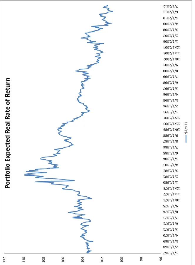
Figure 3 Expected Real Rate of Return on Asset Portfolio ... 54

Figure 4 Risk Adjusted User Cost for Currency, Traveler's Checks, and Demand Deposits ... 55

Figure 5 Risk Adjusted User Cost Other Checkable Deposits ... 56

Figure 6 Risk Adjusted User Cost Savings (without Money Market Demand Accounts) ... 57

Figure 7 Risk Adjusted User Cost Money Market Demand Accounts ... 58

Figure 8 Risk Adjusted User Cost Savings Accounts (with Money Market Demand Accounts) 59 Figure 9 Risk Adjusted User Cost Money Market Mutual Funds (Retail and Institutional) ... 60

Figure 10 Risk Adjusted User Cost Small Denomination Time Deposits ... 61

Figure 11 Risk Adjusted User Cost Large Denomination Time Deposits and Three Month Treasury Bills ... 62

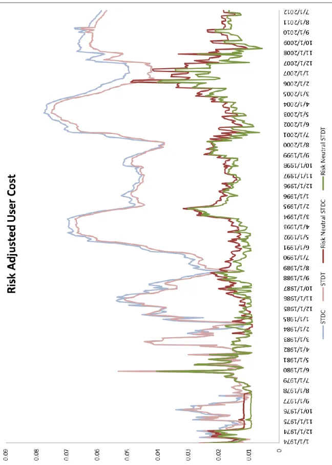
Figure 12 Risk Adjusted User Cost Commercial Paper and Overnight Repurchase Agreements 63 Figure 13 Portfolio User Cost, Certainty Equivalent and Estimated Risk Adjusted. ... 64

Figure 14 Estimated Risk Price Adjustment ... 65

Figure 15 Risk Adjustment for Currency, Travelers Checks, and Demand Deposits ... 66

Figure 16 Risk Adjustment for Other Checkable Deposits ... 67

Figure 17 Risk Adjustment for Savings Accounts (Without Money Market Demand Accounts) 68 Figure 18 Risk Adjustment Money Market Demand Accounts... 69

Figure 19 Risk Adjustment for Savings Accounts (With Money Market Demand Accounts) .... 70

Figure 20 Risk Adjustment for Money Market Mutual Funds ... 71

(11)

xi

Figure 22 Risk Adjustment for Large Denomination Time Deposits, Overnight Repurchase

Agreements, Commercial Paper, and Three Month Treasury Bills ... 73

Figure 23 Risk Adjusted and Risk Neutral Divisia M4 Year-over-Year Growth Rate ... 74

Figure 24 1980 to 1982 GARP Violations ... 92

(12)

1

Chapter 1: Introduction

In the study of macroeconomics a representative agent is constructed to reduce the multiple dimensions associated with an entire population of individual agents with their own preferences and resources. The agent is assumed to consume all goods and services available in some amount; consumption goods, financial assets, and services to monetary assets for example. These components are assumed to be weakly separable in order to aggregate to macroeconomic indicators such as personal consumption expenditures, monetary aggregates, and financial assets. Separability of these components is often assumed without further investigation: currency and travelers checks can be aggregated as “money”, apples and pears as “fruit”, or haircuts and restaurants as “services”. There exists a broad literature testing for weak separability of goods to support the assumption, part of which relies on an assumed functional form of the utility function (the parametric approach) and part on a non-parametric estimation of the data which does not assume a functional form. The use of monetary aggregates relies on its weak separability from consumer goods and financial assets; “money” supplies a service over and above its gross return and acts as a means of exchange providing liquidity service to agents. If weak separability does not hold, there is no utility maximization of the representative agent and therefore no aggregation admissible by economic theory.

The implicit assumption of the weak separability of components in the new Center for Financial Stability’s (CFS) broad Divisia aggregates is tested using recent developments in non-parametric weak separability testing and user cost risk adjustment. The CFS constructs broad Divisia monetary aggregates Divisia M4, Divisia M4-, and Divisia M3 (see

(13)

2

Table 1 Divisia M4, Divisia M4-, Divisia M3 Components) according to the methodology in Barnett, Liu, Mattson and Van den Noort (2013), without adjusting for risk. A more detailed description of this new data set is provided later in this introductory chapter. Chapter 2 examines these components according to the theory developed in Barnett and de Peretti (2009) using the test originally developed in Varian (1982, 1983) and adjusted for stochastic noise so that it does not over-reject1 weak separability due to measurement error or other non-structural factors. The test is advantageous in that does not require the justification of any form of the utility function and instead relies on the microeconomic theory of Revealed Preference. An adjustment to the sufficient weak separability condition in Barnett and de Peretti (2009) is also useful in that it provides a necessary and sufficient condition for admissibility. No narrow aggregates show evidence of admissibility while the broad aggregates pass necessary conditions. In the case of Divisia M4 the necessary and sufficient condition is passed.

Chapter 3 adjusts the user costs of the CFS’ broad Divisia aggregates for risk inherent in the added components: commercial paper, large time deposits, overnight repurchase agreements, and short term treasury bills. The risk adjustment uses a simple conditional capital asset pricing model (CAPM) familiar to the financial literature. The risk adjusted Divisia M4 aggregate is shown to be similar in many time periods to the risk neutral (see Figure 23 Risk Adjusted and Risk Neutral Divisia M4 Year-over-Year Growth Rate), however the user cost prices show relatively large differences. Barnett and Wu (2005) predicted the larger adjustment relative to previous estimations using an unconditional CAPM, such as Barnet, Liu, and Jensen (1997), due to the risk price and risk adjustment in the conditional CAPM. The larger user cost adjustment affects the admissibility testing as it depends on expenditures on components.

1

(14)

3

The results of Chapter 4 suggest that risk adjusted user costs improve the performance of Divisia M4- and maintain support for Divisia M4 in admissibility tests with the exception of the period from 1974 to 1982, specifically the months between March 1980 and November 1982. Test are displayed in the tables and figures and reviewed in the text. Narrower aggregates still fail admissibility in all time periods. The cases for the failure of Divisia M4 in the 1974 to 1982 are considered in light of changes in Federal Reserve policy during the time period of the most significant violations and the large revision in survey methodology that introduced two new types of savings accounts to the monetary aggregates. While the risk adjusted Divsia M4 does not pass the necessary conditions as set out by the Generalized Axiom of Revealed Preference for early 1980s, it does for each time period after. The necessary and sufficient admissible result holds in the risk neutral and risk adjusted case for Divisia M4 from 1982 to the present with the exception of a unique and strong violation in the turbulent months of the financial crisis of 2008 in the risk adjusted case. The suggestion for the macro econometrician then is to use a broad Divisia monetary aggregate in lieu of narrow aggregates which do not show evidence of admissibility and to adjust user costs for risk.

The CFS Advances in Monetary and Financial Measurement Data Set

The following section is a detailed review of the material printed in Barnett, Liu, Mattson and van den Noort (2013) and linked to the CFS’ Advances in Monetary and Financial

Measurement broad Divisia monetary aggregate data set. The CFS produces broad Divisia monetary aggregates in the interest of encouraging monetary economics research, providing alternative monetary measures in a zero-interest rate environment, and allowing for transparent discourse on construction of aggregates and aggregation methods. Data that can be provided on the CFS website is available while data that cannot be directly uploaded to the website is available through other sources such as Wrightson ICAP, Bloomberg, the St.Louis Federal

(15)

4

Reserve Banks Federal Reserve Economic Data (FRED), and Bankrate.com. To further encourage transparency, replication, and open discourse the CFS makes available a document describing all data sources and transformations on its website2.

The construction of broad Divisia monetary aggregates begins with the seminal work by Barnett (1980) and collected in Barnett and Serletis (2000). The first step is to determine the user cost price of holding some monetary asset as opposed to holding on to another. This user cost is the familiar opportunity cost from introductory economics (“you give up something in order to get something”) measuring the liquidity service provided by holding some other less liquid monetary asset with higher returns. It is imperative to understand that the user cost of a monetary asset is not the interest rate paid to that monetary asset. While interest is the user cost of a

financial asset that provides no liquidity, the monetary asset acts not only as a store of value but as a means of exchange; the latter not being taken into account in a simple interest rate. Interest rates, however, are necessary for construction of the user cost as they determine the return on the asset. The definition of the user cost of a monetary asset, in terms of the gross real return defined as where is the real interest rate on some monetary asset observed at time

is _{for some benchmark rate}

. To re-state, the user cost is defined as the opportunity cost for holding some monetary asset that provides a liquidity service over some benchmark asset that provides less liquidity and higher return.

The choosing of the benchmark return is not trivial. Anderson and Jones (2011) use a maximum envelope method, where the highest possible return among a collection of monetary assets and comparable illiquid assets. In some cases the benchmark asset is chosen from among the monetary assets and a zero user cost is produced, which would disrupt the calculation of the Divisia index. To adjust for the case of a zero user cost, 100 basis points are added to the

2

(16)

5

benchmark return to ensure a non-zero and positive user cost. Alternatively a bank loan rate could be considered in the maximum envelope set. Since a bank never gives more in interest than the rate that it charges for loans, the benchmark return is assured to be above the user cost of all monetary assets considered. This method follows the research of Offenbacher and Schachar (2011) at the Bank of Israel in their calculation of Divisia monetary aggregates. The CFS adopts the use of the bank loan rate, more specifically the Weighted Average Effective Loan Rate for Commercial and Industrial Loans, Low Risk provided by the E.2 Survey of Terms of Business Lending. The bank loan rate is quarterly and paired with monthly data, so an expansion method must be used to pair the data3. There has only been one month in the CFS data set where the bank loan rate (when available) has not been the maximum, and it was surpassed by a secondary market large denomination certificate of deposit return, not paired with any of the monetary assets under consideration4. Given the component returns and the return on the benchmark asset (whether it is an actual asset or not) the user cost is easily derived.

After calculation, the user costs are paired with the level of the corresponding monetary asset. The aggregate component levels are defined as and include monetary assets such as

currency, traveler’s checks, demand deposits, savings accounts, small denomination time deposits, and money market mutual funds. The Federal Reserve Board provides simple sum monetary aggregates that include all of these components under the designation M2, and the St. Louis Federal Reserve Bank provides a Monetary Services Index of M2 which is a Divisia share-weighted index. The broader Divisia aggregates provided by the CFS include large denomination time deposits and overnight repurchases that were all once available in the Federal Reserve Board’s M3 simple sum monetary aggregate. Since the M3 component survey is no longer

3

Alternatively one could aggregate the monthly data into quarterly data. 4

It is also most likely an artifact of the quarterly to monthly transformation of the loan rate while the secondary CD rates are all updated monthly.

(17)

6

provided, the assets are collected through other surveys: the Federal Reserve Board’s H.8 Assets and Liabilities of Commercial Banks and the New York Federal Reserve Bank’s Primary Dealers Survey (overnight repurchase agreements). The CFS collects data from these surveys in order to construct their broad aggregates; however the CFS takes the aggregate a little further than the traditional M3 construction, including commercial paper short term Treasury bills in its most broad aggregates. Commercial paper comes from the Federal Reserve Board’s Survey of

Commercial Paper and the Treasury bill amounts and rates are taken from the Monthly Statement of Public Debt. The return and level data are now collected and the actual calculation of the Divisia monetary aggregate can proceed in a few last steps.

The Divisia monetary aggregate is a share weighted index, where the weights on each component are determined based on the total expenditure on that asset. With the user costs and levels, the total expenditure is derived and the share of that expenditure on a particular asset in a given time period is solved using a simple share formula _∑

. To get the

Tornqvist-Theil approximation of Divisia, the average share of the previous and current time period is the weight imputed to each component which can be solved given the previous time periods

share ̅ . Given the user costs, the share weights, and the levels the derivation of the

Divisia index using the Tornqvist-Theil approximation is the solution of the difference equation: ∑ ̅( ( ) ( )).

The series must begin with a normalization of the first period to a value of 100, and the most important information comes from the growth of the Divisia monetary aggregate, not the level. The growth of the Divisia aggregate for the CFS is calculated on a year-over-year basis to avoid seasonality and provide less volatile but still informative analysis. If the growth of the Divisia monetary aggregate is above zero, then the supply of monetary services in the economy is

(18)

7

growing. If the aggregate growth falls below zero, the monetary services in the economy are contracting. Numerous macroeconomic implications from these two simple analyses are drawn regarding growth of GDP, inflation, unemployment, liquidity, and so on. A monthly analysis of recent trends is prosted by the CFS, though the primary goal is to provide the data for open analysis and discourse by researchers, economists, central bankers, and anyone interested in monetary economics.

As in most data base construction projects a certain amount of data transformation occurs to account for seasonality, the termination and beginning of new surveys, and the entry and exit of assets. Those components not already seasonally adjusted by the Federal Reserve Board such as overnight repurchase agreements, commercial paper, and short term treasury bills are adjusted using an X-12 ARIMA process in SAS (see the Code section). The change between surveys of commercial paper is accounted for by using the growth rate trends in the current survey and back-casting those values over Commercial Paper collected in the previous survey. The method is similar for overnight repurchase agreements and large denomination time deposits which were discontinued in the surveys constructing the M3, but not discontinued in other individual surveys with differing methodologies. In order to estimate missing values for interest rates, other

comparable interest rates in the current time period are found a simple linear regression is estimated to back estimate the missing data. The CFS uses these methodologies to derive broad Divisia monetary aggregates back to 1967.

In addition to the usual long term survey issues, the presence of Retail Sweeps severely biases the narrow aggregates. Retail Sweeps are an accounting trick used by banks to

misrepresent the amount of checking balances on their books by “sweeping” those funds into money market demand accounts and counting them as “savings”. The miscalculation of demand deposits allows the banks to hold less legally required reserves. The data survey for M1 is taken

(19)

8

after these sweeps have taken place, and therefore the M1 is biased downward by a catastrophic amount: Barnett (2012) estimates the bias at approximately half the level of M1. The survey taken by the St. Louis Federal Reserve which allows for a sweeps adjustment of narrow aggregates was oddly discontinued in May of 2012, so an estimation procedure based on the interest rate now paid on required reserves is used. While this procedure is now used for the CFS broad Divisia data set, its implementation followed the publication of the data and methodologies paper; it is unfortunately not available in the publication Barnett, Liu, Mattson, and van den Noort (2013). Therefore we now outline the procedure for estimation here. Let be the ratio of swept deposits over total deposits (being the sum of deposits not swept and deposits swept, . Let _{be the opportunity cost of required reserves derived from the}

difference in the benchmark return and required reserve return. The ratio of sweeps to total deposits is estimated and calibrated (the constant ) by simple linear regression of the opportunity cost of required reserved and the level of sweeps recorded by the St. Louis Fed before its discontinuation from November 2008 to March 2012, for before the discontinuation and for afterwards:

_,

̂ ̂ _.

The estimation of sweeps is solved according to the formula from April 2012 and onward, using:

̂

̂ ̂ .

For more details on Retail Sweeps programs see Anderson and Rasche (2001). Unfortunately as the data provided by the St. Louis Fed is no longer available, sweeps estimation must be used to account for the tremendous bias inherent in narrow aggregates that do separate checking

(20)

9

motivation to avoid use of the narrow aggregates above and beyond the analysis of Chapters 2 and 4 on admissibility of aggregates to “go broad”.

A more in-depth analysis of the CFS broad Divisia aggregates is available both on their website and in Barentt, Liu, Mattson, and van den Noort (2013). The grouping of the broad aggregates however into sub-aggregates is given more of an intuitive justification than a rigorous economic justification; these are the clusters that have come before and they are familiar to the typical introduction to economics alumnus. This project seeks to lay a foundation for those clusters through the use non-parametric statistical tests based on the economic theory of Revealed Preference. Furthermore the user costs employed by the CFS are not adjusted for the risk inherent in the broad aggregate components such as overnight repurchase agreements and commercial paper. We adjust those user costs for risk using asset pricing models as developed in Barnett and Wu (2005). Finally, the project concludes with determining the admissibility of clusters in a risk adjusted user cost case. The project builds on the new, foundational data set for broad Divisia monetary aggregates, which provides fertile ground for future research in

(21)

10

Chapter 2: Testing Admissibility in the Risk Neutral Case.

Summary

Chapter 2 defines the theory underlying the development and construction of broad Divisia aggregates for the United States as provided recently by the Center for Financial

Stability. The stochastic semi-nonparametic test for weak separability of clusters by Barnett and de Peretti (2009), based on the Varian (1982) is applied to the new broad Divisia aggregates described in Barnett et al (2012). The test supports the use of the broadest possible cluster of monetary components, Divisia M4 and its sibling Divisia M4- (excluding Treasury bills), but does not support the narrower Divisia M3 cluster. Forms of Divisia M2 are rejected as well, including variations on Divisia M4 and Divisia M4-, with the exception of a Divisia M4 aggregate that excludes Retail Money Market funds in the most recent time period.

(22)

11

Introduction

Chapter 2 identifies admissible clusters of monetary aggregates for the United States using the nonparametric, necessary and sufficient, stochastic method developed in Barnett and de Peretti (2009). The definition of “admissible” comes from Barnett (1982), in that an aggregate is “admissible as an indicator” if composed of a weakly separable cluster of components. For the relevant theoretical background on the necessity of weak separability for the existence of aggregates see Barnett (1980, 1982)5 and the functional structure literature exposited Barnett and Binner (2004).

The test is a recent branching of the nonparametric revealed preference literature. This literature begins in earnest with the three seminal papers Varian (1982, 1983, 1985) which develop a test for satisfaction of revealed preference relations in observed data sets, namely the satisfaction of the Generalized Axiom of Revealed Preference (GARP). Swofford and Whitney (1987) and Fisher and Fleissig (1997) pushed the literature forward theoretically and empirically while Barnett and Choi (1989) pointed to the tendency for over-rejection in the presence of insignificant stochastic errors. A stochastic adaptation of the original Varian (1982, 1983) procedure was necessary. Several approaches developed such as Fleissig and Whitney (2003), Jones et al (2005), Swofford and Whitney (1994), and de Peretti (2005, 2007). The Barnett and de Peretti (2009) test builds on this literature, and then reaches outside the Afriat inequality index method, for a weak separabilty test based on the equality of the marginal rate of substitution and price ratio of goods. The price ratio weak separability test is advantageous as it is both a

necessary and sufficient condition for weak separability if GARP holds.

In 2012 the Center for Financial Stability (CFS) began to provide broad Divisia monetary aggregates and their quantities and user costs of their components to the public. The CFS

5

(23)

12

program, Advances in Monetary and Financial Measurement (AMFM) provides three broad aggregates, Divisia M4, Divisia M4-, and Divisia M3, made up of fifteen separate components6 including currency, travelers checks, demand deposits, interest bearing deposits, savings accounts, small and large time deposits, retail and institutional money market mutual funds, commercial paper, overnight repurchase agreements, and short term treasury bills from 1967 to 20127. The construction methods and data sources for these aggregates are described in Barnett et al (2013). After defining and developing the definition and construction of broad Divisia aggregates in a risk neutral context, the weak separability test in this chapter examines Divisia M3, Divisia M4- and Divisia M4 provided by the CFS and some of the narrower aggregates to determine if they are indeed “admissible” as defined by the theoretical literature. We find evidence for the admissibility of Divsia M4, the broadest aggregate when compared with real personal consumption expenditures; however narrower aggregates such as Divisia M2 and Divisia M3 do not pass these tests.

The User Cost of Money

The Divisia monetary aggregate literature begins with Barnett (1978, 1980) which is reprinted with a near exhaustive amount of complementary papers and research in Barnett and Serletis (2000) regarding the theoretical foundations and empirical evidence of its superiority over other monetary aggregates. Despite the overwhelming evidence of the utility and sense in using an aggregate that does not assume all monetary components are perfect substitutes many central banks insist on using the severely flawed simple sum aggregate, which has been known as far back as Fisher (1922) to be “the worst” aggregate to use in nearly every case. The key difference between the worst and best aggregate being the user cost of money, derived by Barnett

6

The chapter combines currency and travelers checks into one component. 7

(24)

13

(1978), which is the opportunity cost of holding one form of money, say currency, instead of retail money market funds; two clearly different components which should in no case be treated as perfect substitutes.

The user cost (price) is derived in a straightforward manner using the return of the monetary asset and a benchmark rate “given up” in favor of the asset in question. With the user cost price now available, each asset can be weighted in terms of expenditure for a given time period. The expenditure share weights are then used to determine the Tornqvist-Theil

approximation of the Divisia monetary aggregate8. For some asset i=1,…,L and time observation t=1,…,T the gross rate of return9

, quantity , benchmark gross rate of return ,

expenditure share weight and ̅ ⁄ , and aggregate the Divisia aggregate

can be constructed by solving for the user cost, the share weight, and the Tornqvist-Theil approximation respectively: , _∑ , ∑ ̅ ( ( ) ( )).

With the Divisia aggregate solved, one can then determine the dual aggregate user cost for the cluster, , using Fisher’s Factor Reversal.

,

.

8

For a more rigorous theoretical treatment, the reader is referred to Barnett (1980) re-printed in Barnett and Serletis (2000), or for an empirical approach on US data Barnett, Liu, Mattson, and van den Noort (2013). A wealth of literature on international applications of Divisia can be found on the Center for Financial Stability’s website: http://www.centerforfinancialstability.org/amfm_data.php

9

(25)

14

Using this method broad Divsia monetary aggregates are constructed and made available on by the Center for Financial Stability’s program Advances in Monetary and Financial

Measures (CFS). The aggregates and their components are freely available on the CFS website. For a more complete coverage of data sources and methodology, see Barnett, Liu, Mattson and van den Noort (2013).

Weak Separability Testing

Proper clustering of monetary components within an aggregate relies on the Generalized Axiom of Revealed Preference and the condition of weak separability. Let i be the observations of L monetary components. Define the following for the observation at time and component asset :

matrix of observed real per capita monetary quantities,

the th row of ; a vector of real per capita monetary assets,

the matrix of the user cost of holding monetary asset at ,

be the th row of ; the corresponding user costs of at 10.

Pairing these quantities and user cost prices constructs the monetary data set of levels and users costs represented by the sequence { }. Let be partitioned into _a

matrix with and _{a matrix with the corresponding partitions of the user cost}

matrix _and _. _{can then be defined as weakly separable. If there exists an overall}

utility function , a strictly increasing macro function , and a sub-utility function

10

The theoretical procedure outlined in Barnett and de Peretti (2009) works for any real per capita quantity data, and is represented by a matrix of real per capita expenditures and the corresponding price matrix . Since this paper deals specifically with monetary asset components and their user cost, the notation is changed to and to reflect the use of monetary assets and their associated user costs in the Divisia literature collected in Barnett and Serletis (2000).

(26)

15

which admits the following rewriting of the overall utility function then _{is weakly separable}

from _if:

(1) , , (2) .

Furthermore the weak separability of the component vectors implies that the marginal rate of substitutions between any components and within the separable group is independent of changes in those goods outside the group, that is . More formally, for , for , (3) ( ) ⁄ _.

The nonparametric weak separabiltiy literature, beginning with Varian (1982) and Varian (1983) disregards the marginal rate of substitution identity by checking for the existence of the overall utility, the macrofunction, and the sub-utility using the Generalized Axiom of Revealed Preference (GARP). If the overall utility and sub-utiltiy are to exist within the dataset

{ } they must satisfy GARP, i.e. they must behave in a utility maximizing way. The Varian (1982) procedure begins with testing the observed data for satisfaction of GARP. To properly define GARP, we need to define the standard binary relations from microeconomic theory. Consider as before the bundle of real per capita monetary assets at two observations and . Direct revealed preference of to , , means the expenditure at on its asset bundle is strictly greater than the expenditure on any other bundle using prices at ;

. An asset bundle at observation t, , is directly revealed preferred to , , if . Finally, is revealed preferred to , , if a transitive closure

(27)

16

exists between the observations or . GARP is then formally defined for the data set as:

DEFINTION GARP. Data set { } satisfies the general axiom of revealed preference if for observations and the revealed preference of t over s, , implies that the other is not strict directly revealed preferred to the former; “not ”.

Alternatively, using the inequality of expenditure definitions above, GARP can described as satisfied for some data set { } if for all observations,

implies . With GARP well defined, as in Varian (1982), the key theorem for non-parametrically testing weak separability is proposed as:

THEOREM Varian (1982). For the observed data set { }, the following are

equivalent: (i) An overall utility function exists, is locally non-satiated, and rationalizes the data, (ii) there exist marginal income indexes and strictly positive indexes that satisfy the Afriat inequalities, , for any , and (iii) the generalized axiom of revealed preference holds for { }.

Based on Theorem 1, checking for weak separability involves the determining if the data satisfies all of the following three conditions:

CONDITION 1. { } satisfies GARP ( exists). CONDITION 2. {( )}

(28)

17 CONDITION 3. {(( ) ( _))}

satisfies GARP, where and are strictly

positive indexes satisfying the Afriat inequalities , implying {( )}

is weakly separable in .

As described in Barnett and de Peretti (2009) and Fleissig and Whitney (2003) Condition 3 suffers the disadvantage of being a necessary but not sufficient condition for weak separability and the test depends on the method of computing the Afriat inequalities. Adding to the problems associated with Condition 3, Barnett and Choi (1989) prove through Monte Carlo simulations from a pre-determined, admissible functional form of the utility that any single violation of GARP leads to rejection of weak separability, even if the violation is caused by measurement error or stochastic factors. Starting with a modification of Condition 3 that is necessary and sufficient, Barnett and de Peretti (2009) outline a method to resolve these problems, as well as deal with over rejection in the Varian (1982) test.

Assume for now that { } and {( )}

are consistent with GARP (that

Condition 1 and Condition 2 hold). Recall from Equation (3) that the independence condition of the marginal rate of substitution between two assets of a separable group and any assets existing outside that group is necessary and sufficient for weak separability to hold. The unknown form of the utility function is a drawback to this procedure, however if GARP does hold for

{ }, then there is a sub-utility that rationalizes the data by Theorem 1, _._That

is, _{is behaving as a utility maximizing function, and by microeconomic analysis the}

ratio of the prices gives the marginal rate ofsubstitution between assets. (5)

( ) ⁄ ( ) ⁄ .

(29)

18

See Barnett and de Peretti (2009) Lemma 1 for a formal treatment of this condition. Given a maximizing sub-utility function as assumed from the satisfaction of GARP by { } and {( )}

, at first-order conditions the ratio of prices between two assets and are

equal to the corresponding marginal rate of substitution between those two assets. A necessary and sufficient Condition 3 is a test of independence between the price ratios of two goods within the cluster to be checked with the level quantities of those assets outside the cluster.

A regression set up is required, following the method in Barnett and de Peretti (2009). Stack the price ratios of the clustered group into a newly defined vector Y, a ∑

for the th column of the clustered group’s prices matrix _and

. [ ( ⁄ ) ( ⁄ ) ( ⁄ ) ( ⁄ ) ( ⁄ )] .

Define the matrix of quantities _{. Note that} _{can be re-written given the}

clustered group of assets _, ₍ _{) (} _{). Let be the ∑}

vector of residuals, and [ ] be the corresponding vector of parameters. The test for weak separabilitiy would then consist of running the estimation on the following regression

(30)

19 (6) [ ] [ ∑ ] .

then checking if the parameters of the assets outside the cluster are all equal to zero: (7) _∑

_.

The three conditions based on the Varian (1982) theorem are then re-written formally as:

CONDITION 1. { } satisfies GARP ( exists). CONDITION 2. {( )}

satisfies GARP ( exists).

CONDITION 3a. _∑

_{, meaning} _{is weakly separable in .}

Having established a necessary and sufficient weak separability condition using the price ratios of the components within the potential cluster, the problem of stochastic error leading to over rejection in the Varian (1982) test must now be addressed. To properly deal with

stochasticity in the data, begin by setting aside the assumption that data are perfectly observed. Data is now be subject to two assumptions regarding the true data generating process observed with noise, and an assumption regarding variance and stability properties of the distribution of that noise. Let be the matrix of observed monetary quantity data, such that the elements of the matrix are with observations and components . Define as the true component level generated by a weakly separable utility function under the null hypothesis there exists a weakly separable data generating function. The first assumption dictates that the

observations are produced by the addition of the true null matrix with an independently and identically distributed, mean zero error term :

(31)

20

(8) .

The second assumption is that for component the error term is independent and identically distributed with and variance and has a distribution which is max-stable and min-stable; that is all a linear combination of two independent draws of its extreme values has the same location and scale parameters of the original distribution.

Less formally these assumptions dictate that violations of GARP found when testing the subutlitity and macro utility could be due to stochastic factors in the data; i.e. error in

measurement. If these violations are not significant than the Condition 3a weak separability test can follow using the regression model (4) with smoothed quantity level instruments. However if these violations are not significant the cluster must be rejected. Advantageously, the stochastic version of the test does not over-reject as noted in Barnett and Choi (1989) if noise is identified correctly.

The two step iterative procedure developed in de Peretti (2005, 2007), and Barnett and de Peretti (2009) follows a clear logical path in dealing with the stochasticity of the data: first find the minimal adjustment that is need for the data to satisfy GARP in the sub and macro utility functions, then test if the adjustment is significant at an acceptable level. The process is begun by solving for , the minimal adjustment, in the quadratic program subject to the constraints determined by the definition of GARP:

(9) ∑∑

for every and ( ) subject to (C.1) ,

(32)

21

Given the solution matrix to the optimization of (9), ̂, the matrix of theoretical residuals ̂ ̂, is the minimal adjustment need to satisfy GARP for the Condition 1 and Condition 2 restraints; C.1 and C.211. The theoretical residuals matrix ̂ should then be compared to the true measurement error as defined by the difference of the observed sequence of monetary asset quantities and the true sequence of monetary asset quantities: ̂ . Both residual matrices are . Only those bundles that violate GARP are adjusted, meaning only a few can be tested for significance. As this is the case the procedure is to test if the extremes of the theoretical residuals are consistent with the noise created by measurement error. If the extremes of ̂ are significantly outside the possible extremes of ̂ then the GARP violation is significant and the cluster is rejected.

Define the extreme values of the theoretical and true residuals as follows. For and ( ̂ ̂ ̂), the th column of ̂, let ̂ ( ̂ ̂ ̂) and ̂ ( ̂ ̂ ̂ ) be the assumed stable maximum and minimum for the theoretical

residuals. Similarly for the th column of the true residual matrix ̂ to be ( ) and the stable maximum to be ( ), and the minimum is simply

( ). If Assumption 2 holds and these minima and maxima are indeed stable, then the Fisher-Tippett theorem holds:

THEOREM Fisher-Tippett. For ( )an independently and identically distributed sequence, and existing norming constants and and a nondegenerate distribution function such that

(10) → ,

11

(33)

22 then G belongs to one of the three laws:

(10.III) Frechet (type III): for , {

(10.II) Weibull (type II): for , {

, (10.I) Gumbel (type I): for , , .

If there is some prior information regarding the true distributions of errors then using the Fisher-Tippet Theorem, one could determine the law of extremes and choose between the Frechet, Weibull, or Gumbel types. For simplification, we assume the errors behave according to a Guassian distribution, leading to the use of the Gumbel type law12. Using the Gumbel type law, the tail areas for the significance test can be computed according to the p-value for the maxima:

(11) [ ( )], and the p-value for the minima:

(12) [ ( )],

Where ( ̂ ) and ( ̂ ) . What is left is to

calculate the location parameters and as well as the scale parameters and for the distribution . In practice however, the true residual distribution is not

observable except in a small minority of cases. An estimation of is required to continue with the procedure to determine the location and scale parameters and test the extreme values.

Two methods are proposed in Barnett and de Peretti (2009) regarding the estimation of the true residuals, both involving the use of state-space models. Equation (6) from Assumption 1 is just one form of a time invariant state-space model of the form:

12

Another more general method using the Generalized Extreme Value distribution is suggested in Barnett and de Peretti (2009), equation 19 for the form, and Hosking, Wallis, and Wood (1985) and Hosking (1985) for parameter estimation methods.

(34)

23

(13)

In this case is the unobserved level of monetary assets, and are uncorrelated errors. The variances and , , and are the hyperparameters. If and then the model is linear with a trend. If the residuals are assumed to be drawn from a Gaussian distribution, and ̂ is the maximum likelihood estimator of the variance of then the

theoretical residuals can be estimated using the minimum adjustment of residuals ̂, the location and scale parameters, and aforementioned maximum likelihood estimator of the variance of the true residuals. Using Geugan (2003) if we assume to follow a Gumbel type law, the maximum of a series of draws has location and scale parameters defined as:

(14) ( ) [

( ) ]

(15) ( )

As assumed earlier the distributions of the residuals are assumed to be min and max stable, meaning the extreme value distributions has identical location and scale parameters;

and . and are estimated by

̂ ̂ ( ̂ ̂ ̂ ̂ ̂ ̂ ),

̂ ̂ ( ̂ ̂ _̂

̂ ̂ ̂ )

The Condition 1 and Condition 2 test are prepared with the tools described in this section. After running a Kalman filter on the series of monetary asset quantities, the estimation of

variance for the true residuals as well as a smoothed series of asset levels is retrieved. The estimated variance is then used to find the tail areas for the significance test as described above,

(35)

24

and the smoothed values of the levels can be used as instruments for the Condition 3 regression test.

The theoretical background of this test is grounded in the Varian (1982, 1983)

nonparametric weak separability test. Building on the literature of de Peretti (2005, 2007), and Barnett and de Peretti (2009), a stochastic element is introduced to the procedure as well as a necessary and sufficient test for the final condition of weak separabilty, determined by the dependence of user cost price ratios within the cluster to changes in quantity levels of

components outside the cluster. The following section describes the data used and the results that followed.

The Center for Financial Stability and Data Sources

User cost and quantity data for all monetary components come from the openly accessible Advances in Monetary and Financial Measures website from the Center for Financial Stability (CFS). User costs are derived as described in Barnett (1980), using the quarterly weighted low risk average effective loan rate from banks to commercial and industrial clients as a benchmark rate, and the own rates of return on the individual monetary assets. These data come from various sources, including the Federal Reserve Board’s statistical surveys, Bankrate.com, iMoney.net, and the US Department of the Treasury. Short term treasury bills and repurchase agreements are seasonally adjusted by the CFS using an X-12 ARIMA procedure. See

(36)

25

Table 1 for an organizational chart of components into the CFS broad Divisia clusters. For a more exhaustive description of the data, see Barnett et al (2012).

To compensate for the addition and subtraction of monetary components from aggregates, such as the introduction of money market mutual funds to monetary measures in 1973, the data is first split into smaller periods, the most current period starting 1991, at which point money market savings accounts and savings accounts are grouped together under “money market accounts and savings” by the Federal Reserve Board. For time periods before 1991 these two components are treated separately and given different user costs.

Traveler’s checks and currency were combined into one monetary asset as the user costs are identical and the rare use of travelers’ checks has made them a small share of the monetary assets available. Demand deposits are kept as a separate asset despite having the same user cost price as currency and travelers’ checks.

In total there were fourteen monetary components considered for the aggregate clusters, as listed in

(37)

26

Table 1. Currency and travelers checks, demand deposits, and other checkable deposits are traditionally considered the most liquid. Savings, small time deposits, and money market mutual funds are considered less liquid, and included in M2. The Federal Reserve Board, having

discontinued M3 in 2006, no longer considers the broader aggregate components. The CFS has included these components in a larger cluster including those components discontinued with M3, large time deposits, overnight repurchase agreements, and large time deposits, in addition to the inclusion of short term treasury bills as another source of possible liquidity.

(38)

27

Table 1 Divisia M4, Divisia M4-, Divisia M3 Components

LIST OF COMPONENTS AND BROAD CFSAGGREGATE CLUSTERS (1991 TO 2012)

Divisia M3 Divisia M4- Divisia M4

Currency and Travelers Checks X X X

Demand Deposits X X X

Other Checkable Deposits at Commercial Banks X X X

Other Checkable Deposits at Thrift Institutions X X X

Savings and Money Market Accounts at Commercial banks

X X X

Savings and Money Market Accounts at Thrift Institutions

X X X

Small Time Deposits at Commercial Banks X X X

Small Time Deposits at Thrift Institutions X X X

Retail Money Market Funds X X X

Institutional Money Market Funds X X X

Large Time Deposits X X X

Overnight Repurchase Agreements X X X

Commercial Paper X X

3 Month Treasury Bills X

Source: The Center for Financial Stability Advances in Monetary and Financial Measures.

Notes: X denotes inclusion of the component in the aggregate cluster.

Results

The broadest aggregate Divisia M4 was first tested for weak separability from personal consumption expenditures13. For this time period the minimum adjustment value suggests an acceptance of GARP for the DM4 components from consumption expenditures. The maximum adjustment value however weakly rejects weak separability only for other checkable deposits at thrift institutions. Indeed this large adjustment occurs in the latest part of the subsample; the last periods for 1982. These violations of GARP coincide with two important issues: the addition of two monetary assets not before used in the clustering of the aggregates with their own quantities and user costs, and the Savings and Loan crisis. The GARP test could be resolved by changing the sample periods to avoid such violations (as is sometime done in the parametric literature), or

13

In this the sequence of observed data can be represented at { } for the observed personal consumption expenditure at

each observation and the corresponding price index . The test for separability of monetary assets from consumption expenditures follows the work of Binner, Bissondeeal, Elger, Jones, and Mullineux (2008) on the construction of Divisia monetary aggregates for the Euro area.

(39)

28

by adjusting for user cost and determining if the volatility of the time period is not captured by a risk neutral user cost derivation.

Aside from interest bearing checking accounts creating violations for the maximum adjustment that satisfies GARP, all other components in DM3, DM4-, and DM4 failed to reject revealed preference. Indeed the only strong rejection for the sub period of 1974 to 1982 comes with the DM3 aggregate, where interest bearing thrift accounts reject GARP with a 0.0033 tail area.

From the end of 1982 to 1991 the absence of GARP is strongly rejected for all components within and outside DM4 aggregate. All components for DM4 and the personal consumption expenditures aggregate clearly fail to reject the axiom. Both DM3 and DM4- are rejected as satisfying GARP with violations that are too significant in their extreme values.

After August of 1991 the Federal Reserve Board stopped measuring money market deposit accounts and savings deposits as separate components. This subperiod consists of the most major revisions to the data series in the changes in how savings deposits are measured. The evidence for revealed preference is strong for this period as all three clusters pass the Conditions 1 and 2 GARP tests, and there is weak evidence for rejection only in DM3. Both the minimum and maximum adjustment tail areas for interest checking at thrifts stay close to a 5% rejection area (.0460 and 0.609 respectively), however all other components point toward admissible clustering. This is the largest sub-period in terms of observations with T=175 monthly data points.

In July of 2006 the Federal Reserve Board discontinued its M3 simple sum aggregate as well as its component data series for Commercial Paper, Overnight and Term Repurchase Agreements, and Large Time Deposits. Repos are now tracked by the New York Fed in their Primary Dealer Survey, Large Time Deposits in the H.8 Survey of Commercial Banks, and

(40)

29

Commercial Paper is accounted for in its own survey by the Federal Reserve Board. Due to this change in data and survey methodology of the components this contemporaneous subsample remains separate from the major revision in August of 1991. It is the shortest sub period with T=75 monthly observations.

The broadest clusters maintain satisfaction of the GARP test. There is evidence of DM3 rejecting revealed preference again in interest checking accounts available from thrifts. The tail area for large time deposits also dropped precipitously in this sub period (0.0936 for the

maximum adjustment and 0.1407 for the minimum adjustment).

Several alternatives to the traditionally clustered Divisia aggregates were tested. The most successful alternatives clusters included variations of inclusion with retail or institutional money market funds. As seen in

(41)

30

Table 1, for the first and second sub periods the an altered Divisia M4 that excluded retail money market funds instead of excluding Treasury bills satisfied the Condition 1 and Condition 2 GARP tests when the DM4- cluster provided by the CFS actually failed both GARP and weak separability from 1982 to 1991. In fact the Divisia M4 excluding retail money market funds satisfies GARP and the weak separability test with similar tail areas as Divisia M3 seems to improve once retail or institutional money market funds are removed from the measure as they satisfy GARP conditions, but still fail the weak separability test.

More narrowly constructed Divisia aggregates using the CFS’ methodology and

benchmark rate in forms similar to MZM, and M2-ALL produced by the Federal Reserve Board in simple sum format. For most sub periods Divsia MZM and Divisia M2-ALL did not satisfy the Condition 1 and Condition 2 GARP tests. When they did they were strongly rejected by the Condition 3 weak separability test. As a comparison the narrower aggregates did not satisfy the requirements of admissibility.

(42)

31

Table 2 Admissibility Test Results

RESULTS OF THE WEAK SEPARABILITY TEST ON BROAD ANDNARROW CLUSTERS

1974-1982 1982-1991 1991-2006 2006-2012 Divisia M4 G**/WS* G*/WS** G*/WS** G*/WS* Divisia M4 Less RMF G** G* G* G*/WS** Divisia M4 Less MMF G** G* G* X Divisia M4- G** X G* G* Divisia M3 X X G** G** Divisia M3 Less RMF G** G* G** G* Divisia M3 Less MMF G** G* G** G* Divisia M2 ALL G** X X G** Divisia MZM G** X X G**

Notes: G denotes failure to reject Conditions 1 and 2, but rejection of Condition 3. G/WS denotes failure to reject all three conditions. X denotes a rejection of all conditions.

Source: Author calculations. ** Significant at the 1 percent level * Significant at the 5 percent level.

Table 3 GARP 1974 Results

TAIL AREA RESULTS OF THE GARPTEST ON BROAD CFSCLUSTERS 1974:1982,T=100

Divisia M3 Divisia M4- Divisia M4 Currency and Travelers Checks .3664 / .2034 .3668 / .2229 .4043 / .3085 Demand Deposits .5936 / .7928 .7011 / .6189 .7182 / .6717 Other Checkable Deposits Comm. .3387 / .6932 .3357 / .6808 .3516 / .6859 Other Checkable Deposits Thrift .0033 / .0921 .0284 / .3362 .0329 / .3460 Savings Less MMDA Comm. .7159 / .8148 .7273 / .8160 .7364 / .8151 Savings Less MMDA Thrift .6232 / .5809 .4244 / .6702 .4479 / .6754 Retail Money Market Funds .8386 / .7888 .6986 / .6666 .6952 / .6385 Small Time Deposits Comm. .8464 / .8052 .8472 / .8071 .8466 / .7722 Small Time Deposits Thrift .7111 / .6819 .8433 / .7990 .8427 / .7604 Institutional Money Market Funds .8647 / .8430 .8046 / .7909 .8031 / .7786 Large Time Deposits .7269 / .6818 .8515 / .8161 .8510 / .7853 Overnight and Term Repos .7043 / .5824 .8176 / .7835 .8367 / .7985 Commercial Paper (.8296 / .8070) .6576 / .6109 .7070 / .6543 Short Term Treasury Bills (.8618 / .8746) (.8870 / .8870) .8191 / .8021

Personal Consumption Expenditures NA NA (.8870 / .8870)

Notes: “Max Tail Area / Min Tail Area”. (Tail Area for Overall Utility Component not in Sub-utility).

(43)

32

Divisia M3 Divisia M4- Divisia M4 Currency and Travelers Checks .5722 / .7053 .6251 / .6375 .7183 / .7983 Demand Deposits .7831 / .8268 .8010 / .8050 .8310 / .8357 Other Checkable Deposits Comm. .2499 / .6234 .3110 / .7612 .7036 / .7359 Other Checkable Deposits Thrift .0063 / .2387 .0129 / .5197 .3736 / .4750 MMDA Commercial .8388 / .8091 .8196 / .8499 .8405 / .8566

MMDA Thrift .8183 / .7741 .7897 / .8340 .8209 / .8434

Savings Less MMDA Comm. .8558 / .8209 .8477 / .8651 .8558 / .8606 Savings Less MMDA Thrift .7946 / .6477 .7673 / .8221 .7950 / .8381 Retail Money Market Funds .7057 / .7483 .7981 / .8466 .7985 / .7560 Small Time Deposits Comm. .8049 / .8270 .8414 / .7609 .8423 / .8302 Small Time Deposits Thrift .7965 / .8210 .8369 / .7478 .8324 / .8245 Institutional Money Market Funds .8079 / .8260 .8498 / .8677 .8493 / .8293 Large Time Deposits .8142 / .8337 .8464 / .7754 .8217 / .8365 Overnight and Term Repos .7482 / .8235 .8228 / .7754 .8675 / .8096 Commercial Paper (.8835 / .8757) .8235 / .7718 .8283 / .8230 Short Term Treasury Bills (.8833 / .8864) (.8875 / .8875) .8783 / .8603 Personal Consumption Expenditures NA NA (.8875 / .8875 )

(44)

33

Divisia M3 Divisia M4- Divisia M4 Currency and Travelers Checks .5272 / .6526 .5757 / .6760 .4899 / .8618 Demand Deposits .7707 / .8132 .7877 / .8207 .6815 / .8807 Other Checkable Deposits Comm. .7558 / .6190 .7806 / .7368 .4533 / .8581 Other Checkable Deposits Thrift .0609 / .0460 .1607 / .1178 .2195 / .5829 Savings and MMDA Comm. .8679 / .8361 .8731 / .8576 .7554 / .8820 Savings and MMDA Thrift .8258 / .8400 .8457 / .8455 .7616 / .8776 Retail Money Market Funds .7689 / .8046 .8078 / .8286 .7584 / .8417 Small Time Deposits Comm. .8383 / .7989 .8592 / .8322 .7902 / .8779 Small Time Deposits Thrift .8309 / .8563 .8453 / .8603 .7804 / .8694 Institutional Money Market Funds .8399 / .8341 .8561 / .8499 .7906 / .8652 Large Time Deposits .7979 / .7533 .8374 / .8024 .7669 / .8634 Overnight and Term Repos .7957 / .7396 .8380 / .8143 .7784 / .8648 Commercial Paper (.8891 / .8897) .8139 / .7707 .7201 / .8655 Short Term Treasury Bills (.8909 / .8908) (.8915 / .8915) .7716 / .8800

(45)

34

Divisia M3 Divisia M4- Divisia M4 Currency and Travelers Checks .4712 / .2766 .4682 / .6865 .3928 / .7409 Demand Deposits .7434 / .6512 .7422 / .8184 .7106 / .8359 Other Checkable Deposits Comm. .5822 / .2737 .5994 / .6674 .4480 / .6891 Other Checkable Deposits Thrift .0211 / .0879 .2521 / .0975 .1784 / .5809 Savings and MMDA Comm. .7494 / .8198 .7487 / .7681 .7239 / .8273 Savings and MMDA Thrift .6369 / .5137 .7209 / .6597 .6679 / .6687 Retail Money Market Funds .4971 / .4361 .5640 / .4357 .5868 / .3987 Small Time Deposits Comm. .7025 / .6669 .7941 / .7957 .7725 / .8020 Small Time Deposits Thrift .1928 / .5868 .5521 / .5120 .7410 / .7210 Institutional Money Market Funds .7261 / .6974 .7562 / .6972 .7649 / .6780 Large Time Deposits .0936 / .1407 .1430 / .3408 .3995 / .3933 Overnight and Term Repos .1360 / .5749 .5571 / .5898 .5545 / .4260 Commercial Paper (.8544 / .6932) .6438 / .5427 .8524 / .5434 Short Term Treasury Bills (.8262 / .8796) (.8843 / .8843) .7944 / .8400

(46)

35

Table 7 Weak Separability Test

TAIL AREA RESULTS OF CONDITION 3WEAKLY SEPARABLE TEST

Cluster Time Period Sample Size MinTail Area

DM4 1971:1982 100 0.1164 1982:1991 105 0.0231 1991:2006 175 0.0131 2006:2012 75 0.0678 DM4- 1971:1982 100 0.0056 1982:1991 105 0.0000 1991:2006 175 0.0060 2006:2012 75 0.0041 DM4 Less RMF 1971:1982 100 0.0027 1982:1991 105 0.0000 1991:2006 175 0.0013 2006:2012 75 0.0401

Notes: The smallest minimum tail area of the price ratios is reported. Tail areas below .01 are immediately rejected while those between .01 and .10 are reported.

(47)

36

Conclusion

The empirical application of a nonstochastic semi nonparametric test for weak separability as outlined in Barnett and de Peretti (2009) points to the admissibility of broad Divisia monetary aggregates, in favor of narrower aggregates. The evidence is weak for the admissibility of narrow monetary components.

The test used in this chapter provides a new branch in the varied literature on non-parametric weak separabilty tests, which stretches back to Varian (1982)’s use of revealed preference as a basis. Stochastic factors are taken into account using quadratic programming and the Kalman filter in order to determine when violations of utility maximizing behavior are significant. The new stochastic version of the GARP test performs well in the empirical context, identifying clusters that are appropriate according to revealed preference. The Condition 3 weak separability procedure examines the relationship between the user cost price ratios of the

monetary components within the cluster and the quantities of those components outside the cluster based on the relationship of the marginal rate of substitution and price ratios. The

rejection of most narrow aggregates, in favor of the broadest aggregate is informative for the use of monetary aggregates in policy and research.

Natural extensions of the research include a test to determine if bonds and securities should be included with in the “monetary cluster”, as well as extensions of Barnett and de Peretti’s (2009) theory to test other possibly admissible clusters of goods. The next important step would be to carry out an analysis of the recent time series of Divisia aggregates would produce interesting results especially during the time period of the 2008 financial crisis and succeeding recession in the spirit of Barnett, Offenbacher, and Spindt (1982). One could also explore the alternative approaches to the Condition 1 and 2 test using different aspects of extreme value theory to test the minimum and maximum adjustments for significance.

(48)

37

Furthermore it should be recognized that the risk environment in the US economy has fluctuated over several periods. An incorporation of the risk-adjusted user cost as proposed in Barnett and Wu (2005) and Barnett, Liu and Jensen (1997) would alter the user costs associated with the components and reveal more information on the structure of monetary assets. In fact most violations of GARP exist during periods of high uncertainty such as the Savings and Loan Crisis and the change in regulation for savings and loan (thrift) institutions, and the recent financial crisis. Finally an incorporation of these admissible aggregates would resolve many of the

problems in macroeconomic models that have so far only used the inferior simple sum measures, often leading to the erroneous conclusion that only interest rates are important to policy and “money does not matter”.

(49)

38

Chapter 3: Deriving the Risk Adjusted User Cost of Money.

Summary

Barnett, Liu, Mattson, and Van den Noort (2012) construct a new data set of broad Divisia monetary aggregates freely available to the public by the Center for Financial Stability. Chapter 2 uses a state of the art methodology developed in in Barnett and de Peretti (2009) to find strong support for the admissibility of the broadest possible aggregate, Divisia M4, over narrower clusters. However these aggregates are not adjusted for risk despite the strong effects of risk on components such as commercial paper and overnight repurchase agreements. This paper details the construction of the broad risk adjusted Divisia M4 and components such as the risk adjusted user cost, the risk price of the representative agent’s asset portfolio, and the risk adjustment for each component asset used in the following chapter. While the risk adjusted Divisia M4 aggregate follows closely with the risk neutral aggregate, the user costs of each component generally become larger and smoother than their risk neutral counterparts.