Procedia Engineering 15 (2011) 199 – 203 1877-7058 © 2011 Published by Elsevier Ltd. doi:10.1016/j.proeng.2011.08.040
Procedia
Engineering
Procedia Engineering 00 (2011) 000–000 www.elsevier.com/locate/procediaAdvanced in Control Engineeringand Information Science
Chaos quantum-behaved particle swarm optimization based
neural networks for short-term load forecasting
Hongsheng Su*
School of Automation and Electrical Engineering, Lanzhou Jiaotong University, Lanzhou 730070, China
Abstract
To tackle with the premature matter of particles when seeking optimization in local small space in terms of quantum-behaved particle swarm optimization(QPSO), chaos optimization strategy was combined to QPSO algorithm, and defined as chaos quantum-behaved particle swarm optimization(CQPSO) algorithm. The algorithm firstly applied QPSO algorithm to implement evolution operation till QPSO algorithm was in premature state, then chaos seeking mechanism was started to induct the particles to quickly jump out the local optimization, and thus, the convergence speed of QPSO was quicken. In this paper, CQPSO was applied to optimal the weight values of BP neural network, and the optimized well neural network was applied to implement short-term load forecasting(STLF). Eventually, simulation results show that the algorithm possesses high forecasting accuracy, and is an ideal optimal algorithm.
© 2011 Published by Elsevier Ltd.
Selection and/or peer-review under responsibility of [CEIS 2011]
Key words: Quantum-behaved particle swarm optimization(QPSO); chaos; neural networks; short-term load forecastting(STLF)
1. Introduction
In power system load short-term forecasting, artificial neural network (ANN) is a frequently used method [1, 2]. Load forecasting using ANN possesses many prominent advantages, but has some
shortcomings, such as slowing converge speed, local converge, and etc, which make prediction results
to be very dissatisfactory. Hence, many improved algorithms are proposed for ANN learning. In [3] ge- * Corresponding author. Tel.: +86-0931-4938656; fax: +86-0931-4938826.
E-mail address: [email protected]
Open access under CC BY-NC-ND license.
-netic algorithm (GA) is applied to optimize the weights of ANN. The algorithm firstly applies GA to generate an initial network, and then, the network is further trained to acquire a final structure using sample data. Clearly, it improves the learning quality of ANN, dramatically. In [4] particle swarm optimization(PSO) is applied to learn the ANN weight values, which overcomes the shortcomings of BP learning algorithm, and achieves a better global approximate capability. However, due to limitation in seeking optimization space, traditional PSO exposes out many flaws, for example, getting into local extremums, easily, slow convergence speed, low classification accuracy, and etc. In [5] quantum-behaved particle swarm optimization(QPSO) is proposed and applied to ANN learning, due to expansion in seeking space, QPSO can achieve a better global solution than PSO. But like PSO, QPSO still exposes some problems in iterative operations such as premature, which result in an earlier standstill of the particles, and make the algorithm lose activities. Based on it, in this paper chaos seeking mechanism is combined into QPSO to generate CQPSO algorithm. The algorithm firstly implements QPSO till premature state, then chaos seeking is started to induct the particles to quickly get rid of the local optimization, and that the convergence of QPSO is improved, dramatically.
2. CQPSO Algorithm 2.1. PSO algorithm
Letn particles in D-dimensional space, the ith particle may be described as a D-dimensional vector xi=(xi1,xi2,…,xiD),i=1,2,…,n, namely, the position of the ith particle in D-dimensional space is xi, and each
such position is named as a potential solution. The adaptability function value of xi is calculated by
substituting it into the aim function f(xi), then, according to the value size, xi can be weighed to be the
good or the bad. The flight speed of the ith particle is also a D-dimensional vector, and expressed as vi=(vi1,vi2,…,viD). Assume that until now the optimal position sought by the ith particle is
pi=(pi1,pi2,…,piD), and the optimal position sought by the whole particle swarm is pg=(pg1,pg2,…,pgD),
which respectively called as pbest and gbest. Then the position and speed of the particle i can be evolved
below. )] ( ) ( 2 2 1 1 1 k id k gd k id k id k id k id v cr p x c r p x v + =ω× + − + − (1) 1 1 + + = + k id k id k id x v x (2) In (1), ωis inertia weight, and indicates an influence yielded by the present speed of the particle on next generation. A suitable ω can make the particle hold balanced exploration abilities. Parameters c1and c2 are non-negative learning factors, the values of which usually are limited in range of one to two, if the
values are too small, the particle is far away from the optimal aim area, inversely, if too large, the particle can suddenly or possibly fly over aim area. r1andr2 are random variables with a scope of zero to one.
2.2. QPSO algorithm
QPSO was proposed in 2004, it made an improvement on PSO from quantum mechanics angle. Based on Delta potential-trap, the model considers the particles possess quantum behavior, and proposes the QPSO. QPSO is a complex nonlinear system, and accords to states superposition principle. Hence, quantum system possesses more states, and is an indeterminate system without determinate tracks, thus each particle can appear in arbitrary position in seeking space according some probability, which is
favorable in terms of the global convergence and shaking off the local extremum. In QPSO algorithm, the position information of the particle can be updated according to the following equations below.
∑
∑
∑
∑
= = = = = = M i M i iD i M i i M i i best M x M p M p M p m 1 2 1 1 1 1 ) 1 , , 1 , 1 ( 1 L (3) * (1 )* id id gd p =ϕ p + −ϕ p (4))
1
ln(
|
|
1u
x
m
p
x
k id d best id k id +=
±
θ
−
(5)where mbest expresses the average optimal position, M expresses the colony size, ϕ* and u is random
number with a scope of zero to one, θ is an expanded coefficient of QPSO, and used to control the convergence speed.
2.3. CQPSO algorithm
CQPSO is based on QPSO, under the precondition that seeking mechanism of QPSO is not changed whether the particles are premature or not by introducing premature judgment mechanism. If premature condition holds in each iterative process, chaos seeking mechanism is started so as to the particles shake off the local extremum, and inversely, and QPSO is implemented according to origin plan. Here typical logistic mapping is applied to generate chaos signal, and is described as follows [6].
(
)
1
1
k k k
x
+=
μ
x
−
x
(6)where u is control parameter, u =4, and while 0<x<1, logistic mapping is fully chaos state. After chaos signal is generated, the optimal variable is carried into chaos state.
The step of the algorithm is below.
Step1. Give the initial position xi(0) of each particle, and individual optimal position pi(0), and global
optimal position pg(0).
Step2. According to (3), calculate the mbest(t+1).
Step3. Calculate the present fitness degree of each particle.
Step4. Update the local optimal value of each particle according to following formula, assume that
aim function be f(x).
Pi(t), if f(Pi(t)≥f(Xi(t+1))
Pi(t+1)= (7)
Xi(t+1), if f(Pi(t)<f(Xi(t+1))
Step5. Update the global optimal value according to following formula.
{
1 2}
( 1) min ( 1), ( 1),..., ( 1)
g
P t+ = P t+ P t+ P tM = (8)
Step6. Compare the global optimal value with the former one, if the current location is better, then the
current position replaces the former one as new optimum.
Step7. In term of each dimension of the particles, update it using (4)
Step8. Update location information of the particle according to (5).
Step9. According to (9) the square error δ2 is calculated out, if δ2<ε, then colony is considered
premature, according to (6) chaos seeking is implemented N times to find optimal value, and the optimal value is served as the optimal solution of the current particles.
2 2 1 1 M i avg j f f M f δ = − ⎛ = ⎜ ⎝ ⎠
∑
⎞⎟ (9)In (9) fi is current fitness degree of the particle, and favg is average fitness degree of the colony, f
is a normal factor, which produce a limitation on δ2. f can be described below.
{
}
{
if
avg}
max 1 max
f
=
,
f
−
(10) where i=1,2,…, M.Step10. Repeat step2 to step10, till one terminal condition holds.
3. CQPSO-BP Learning Algorithm
The CQPSO-BP algorithm is divided as two parts. Firstly, CQPSO algorithm is applied to optimize the weights and thresholds of the neural networks, till the prescriptive iterative times N is reached. BP learning algorithm is then applied to train the networks more deeply, till the desired aim is achieved.
Letd neurons be in input layer, m in hidden layer, and n in output layer, neural networks therefore possess d×m+m×n+m+n weights and thresholds in all. Correspondingly, the dimensions of each particle of CQPSO algorithm should also be d×m+m×n+m+n. Let the network possess N training samples, mean square error (MSE) is then expressed by
MSET=
1
N
1 N i=∑
[ 1 n j=∑
(tij-yij)2] (11)The above equation may serve as the fitness function in CQPSO-BP networks, where tij is the desired
export and yij is the practical output of the network. To evaluate the prediction results, quantitatively, the
following two indexes are applied to test learning algorithms. 1) Relative error rate εr
εr =[|practical_value – predictive_value| /practical_value]×100% (12)
2) Averaging relative error rata εave
εave=(1/M)∑ [|practical_value – predictive_value| /practical_value]×100% (13)
where M represents the number of the checking samples.
4. Eamples
The load data come from one southern city in China in Sep-2009, the load values in full o’clock come from 7th-Sep-2009 to 13th-Sep-2009. Hence, the structure of BP network may be selected as 24-10-24,
whose transfer function of the neurons in middle layer selects S type tangent function tansig, and the one in output layer is S type logarithm function logsig. The reason to do this is that outputs of the functions is within the scope of 0 to 1, output requirements of the networks can just be well satisfied. Learning function is trainlm function. Let the gross number of the particles be 30, the dimension of the particle in CQPSO algorithm should also be 24×10×24+10+24=514, and the maximum learning times Tmax of the
networks be 1000, and the training aim ε be 0.001. After the network training stationary, we may apply the well trained network to implementation load forecasting. In practice, we select the data of the former
day serve as the inputs of the network to forecast the load of load day one times in hour, the acquired predicting values are shown in Table 1.
Table 1. Predicting results analysis of CQPSO algorithm
Seen from Table 1, the CQPSO predicting results are coincided with practice ones better, where the average value of the relative errors is 1.78% alone, and the maximum is 3.6%, and the minimum is zero, and the variable scope of the errors is smaller. To further illustrate the advantages of the CQPSO-BP, QPSO-BP, PSO-BP, and BP algorithm are here adopted to make comparisons using the same data with CQPSO-BP algorithm. The final comparisons are shown in Table 2.
Terms Practical values (Mwh) Predicting values (Mwh) ε (%)
Average value 19.52 19.46 1.78
Minimum 20.15 20.17 0.0
Maximum 20.42 21.17 3.6
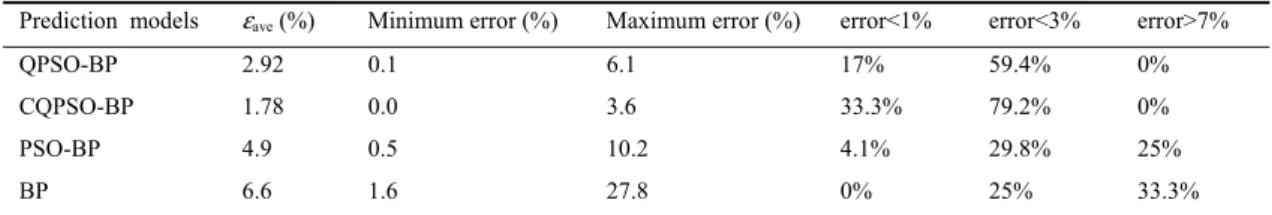
Table 2. Statistic results of four prediction models
Prediction models εave (%) Minimum error (%) Maximum error (%) error<1% error<3% error>7%
QPSO-BP 2.92 0.1 6.1 17% 59.4% 0%
CQPSO-BP 1.78 0.0 3.6 33.3% 79.2% 0%
PSO-BP 4.9 0.5 10.2 4.1% 29.8% 25%
BP 6.6 1.6 27.8 0% 25% 33.3%
From Table 2, we can see the prediction results with CQPSO-BP optimization based are better then ones of other optimization models. This shows that QPSO Algorithm with chaos mechanism introduced possesses better prediction accuracy.
5. Conclusion
The CQPSO algorithm mentioned in this paper acquires desired results in power systems short-term load forecasting. This shows that the algorithm is feasible and ideal in technique, and being expected to put into practice, and achieve good economic benefits.
References
[1] Lee KY, Cha YT. Short-term load forecasting using an artificial neural network. IEEE Transactions on Power System 1992, 7(1):124-132.
[2] Wang K. Short-term load forecasting for special days in anomalous load conditions using neural networks and fuzzy inference method. IEEE Transactions on Power Systems 2000, 15(2):559-565.
[3] Jia ZY, Niu DX. Genetic neural network model of electric power load forecasting. Opration and Management 2000, 9(2):31-36.
[4] Liu L, Zhang HM, Li DP. Short-term power load forecasting based on fuzzy neural network with PSO optimized.
Preceedings of the CSU-EPSA 2006, 18(3):47-50
[5] Kong QQ. Improved QPSO algorithm and its applications. Wuxi: Jiangnan University; 2008. [6] Huang RS, Huang H. Chaos theory and its applications. Wuhan: Wuhan University Press; 2005.