Shan Zhong
Submitted in partial fulfillment of the requirements for the degree
of Doctor of Philosophy
in the Graduate School of Arts and Sciences
COLUMBIA UNIVERSITY
Signal Processing for Wireless Power and
Information Transfer
Shan Zhong
The rapid development of the Internet of Things (IoT) and wireless sensor network (WSN) technologies enable easy access and control of a variety forms of information and data from numerous number of smart devices, and give rise to many novel ap-plications and research areas such as smart home, machine type communications, etc. However due to the small sizes, sophisticated environment, and large number of devices in network, it is hard to directly power the devices from grid. Hence the power connectivity remains one of the major issues that needs to be addressed for related IoT applications. Wireless power transfer (WPT) and backscatter communi-cations are provisioned to be prominent solutions to overcome the power connectivity challenge, but they suffer strong efficiency limitation which becomes the barrier to universally popularize such technologies. On the other hand, network optimization is also a research focus of such applications which significantly affects the performance of the system due to the high volume of connected devices and different features.
In this thesis we propose advanced techniques to overcome the challenges on the low efficiency and network design of the wireless information and power transfer systems. The thesis consists of two parts. In the first part we focus on the power transmitter design which addresses the low efficiency issue associated with backscatter communication and WPT. In Chapter 2, we consider a backscatter RFID system with the multi-antenna reader and propose a blind transmit and receive adaptive beamforming algorithm. The interrogation range and data transmission performance
first present the WPT model for the beamspace MIMO which is derived from the spatial MIMO model. By constraining on the number of RF chains in the transmitter, we formulate two WPT optimization problems: the sum power transfer problem and the max-min power transfer problem. For both problems we consider two different transmission schemes, the multi-stream and uni-stream transmissions, and we propose different algorithms to solve both problems in both schemes respectively.
In the second part we study the network optimization problems in the WPT and backscatter systems. In Chapter 4, we study the resource allocation problem for a RF-powered network, where the objective is to maximize the total data throughput of all sensors. We break the problem into two subproblems: the sensor battery energy utilization problem and the charging power allocation problem of the central node, which is an RF power transmitter that transmits RF power to the sensors. We analyze and show several key properties of both problems, and then propose computationally efficient algorithms to solve both problems optimally. In Chapter 5, we study the time scheduling problem in RF-powered backscatter communication networks, where all transmitters can operates in either backscattering mode or harvest-then-transmit (HTT) mode. The objective is to decide the operating mode of each transmitter and minimize the total transmission time of the network. We also consider both ideal and realistic transmitters based on different internal power consumption models for HTT transmitters. Under both transmitter models we show several key properties, and propose bisection based algorithms which has low computational complexity that solves the problem optimally. The results are then extended to the massive MIMO regime.
List of Figures v
List of Tables viii
Chapter 1: Introduction 1
1.1 Background and Motivation . . . 1
1.2 Outline and Contributions . . . 4
1.2.1 Multi-Antenna Transmitter Design for Backscatter Communi-cation and Wireless Power Transfer . . . 4
1.2.2 Network Optimization for Wireless Power Transfer and Backscat-ter Communication Systems . . . 6
Part I Multi-Antenna Transmitter Design for Backscatter Commu-nication and Wireless Power Transfer 8 Chapter 2: Multi-Antenna Backscatter Reader Design with Blind Adaptive Beamforming 9 2.1 Introduction . . . 9
2.2 Reader Interrogation Range . . . 11
2.2.1 Single-antenna Case . . . 12
2.2.2 Multiple-antenna Case . . . 14
2.3 Blind Adaptive Beamforming for RFID Reader . . . 17
2.3.1 Full-duplex Reader . . . 17
2.3.2 Half-duplex Reader . . . 18
2.4.2 Multiple-antenna Case . . . 21
2.5 Tag Quantity Estimation . . . 22
2.5.1 Single-antenna Case . . . 25
2.5.2 Multiple-antenna Case . . . 26
2.6 Simulation Results . . . 27
2.6.1 Interrogation Range Performance . . . 28
2.6.2 Data Transmission Performance . . . 34
2.6.3 Tag Quantity Estimation Performance . . . 36
2.7 Experimental Validation . . . 36
2.8 Conclusions . . . 41
Chapter 3: Wireless Power Transfer by Beamspace MIMO with Lens Antenna Array 42 3.1 Introduction . . . 42
3.2 System Model . . . 45
3.2.1 MmWave MIMO Channel Model in Spatial Domain . . . 46
3.2.2 Beamspace MIMO with Lens Antenna Array . . . 48
3.3 Maximum Sum Power Transfer . . . 49
3.3.1 Problem Formulation . . . 49
3.3.2 Optimality of Uni-stream Transmission . . . 50
3.3.3 Sum Power Maximization - Algorithm 1 . . . 51
3.3.4 Sum Power Maximization - Algorithm 2 . . . 52
3.4 Max-Min Power Transfer . . . 56
3.4.1 Problem Formulation . . . 56
3.4.2 Multi-Stream Max-Min Power Transfer . . . 56
3.4.3 Uni-Stream Max-Min Power Transfer . . . 58
3.5 Simulation Results . . . 64
3.6 Conclusions . . . 76
3.7 Appendices . . . 77
3.7.1 Proof of Lemma 1 . . . 77
3.7.2 Proof of Theorem 1 . . . 77
Part II Network Optimization for Wireless Power Transfer and Backscat-ter Communication Systems 78 Chapter 4: Energy Allocation and Utilization for Wireless Powered Networks 79 4.1 Introduction . . . 79
4.2 System Descriptions . . . 82
4.3 Problem Formulation . . . 85
4.3.1 Energy Utilization Planning Subproblem . . . 85
4.3.2 Power Allocation Subproblem . . . 88
4.4 Optimal Energy Utilization Policy . . . 89
4.5 Optimal Power Allocation Algorithm . . . 92
4.6 Simulation Results . . . 97 4.7 Conclusions . . . 104 4.8 Appendices . . . 105 4.8.1 Proof of Lemma 2 . . . 105 4.8.2 Proof of Lemma 3 . . . 107 4.8.3 Proof of Theorem 2 . . . 108 4.8.4 Proof of Theorem 3 . . . 110
Chapter 5: Time Scheduling in Wireless Powered Backscatter Com-munication Networks 112 5.1 Introduction . . . 112
5.2 System Description and Problem Formulations . . . 114 iii
5.3 Optimal Solution for Ideal Case . . . 119
5.4 Optimal Solution for Realistic Case . . . 124
5.5 Extensions to Massive MIMO . . . 127
5.5.1 Massive MIMO System Model and Problem Formulation for Ideal Case . . . 127
5.5.2 Optimal Solution for Ideal Case . . . 129
5.5.3 Massive MIMO with Realistic Transmitters . . . 130
5.6 Simulation Results . . . 133
5.6.1 Results for Single Antenna Reader . . . 133
5.6.2 Results for Massive MIMO Reader . . . 137
5.7 Conclusions . . . 138 5.8 Appendices . . . 139 5.8.1 Proof of Proposition 1 . . . 139 5.8.2 Proof of Lemma 6 . . . 139 5.8.3 Proof of Theorem 4 . . . 140 5.8.4 Proof of Theorem 5 . . . 141 5.8.5 Proof of Proposition 2 . . . 142 5.8.6 Proof of Lemma 7 . . . 143 5.8.7 Proof of Lemma 8 . . . 144 5.8.8 Proof of Theorem 7 . . . 145 5.8.9 Proof of Theorem 8 . . . 146 5.8.10 Proof of Theorem 9 . . . 148 Chapter 6: Conclusions 149 Bibliography 150 iv
Figure 1.1 System architecture of energy harvesting transmitters. . . 3
Figure 1.2 Flow diagram of backscatter communication. . . 3
Figure 2.1 (a) A passive full-duplex multiple-antenna UHF RFID system and (b) a half-duplex reader. . . 12
Figure 2.2 Interactions between the reader and the tag. . . 19
Figure 2.3 (a) FM0 symbols and (b) FM0 sequences. . . 20
Figure 2.4 A MIMO RFID protocol with BABF algorithm. . . 22
Figure 2.5 RCS plots based on the reception of the replied RN16s of tags: (a) two tags replying simultaneously resulting in four clusters and (b) three tags replying simultaneously resulting in eight clusters. . . 23
Figure 2.6 The convergence of the proposed BABF algorithm with different values of Kp in full-duplex setting, M = 2. . . 28
Figure 2.7 The convergence of the proposed BABF algorithm with different values of Kp in half-duplex setting, M =N = 2. . . 29
Figure 2.8 Average interrogation range versus number of antennas under full-duplex setting. . . 30
Figure 2.9 Average interrogation range versus number of antennas under half-duplex setting. . . 32
Figure 2.10 Interrogation range in mobile environment. . . 32
Figure 2.11 PER performance in a Rician fading channel (K = 2.8 dB) for different BF schemes. . . 35
Figure 2.14 Experiment layout. . . 38
Figure 2.15 Probability of successful RFID tag reading. . . 39
Figure 2.16 Backscattered signal strength received . . . 40
Figure 3.1 Illustration of the two types of multi-agent systems. . . 47
Figure 3.2 Geometric interpretation of the RCG algorithm. . . 62
Figure 3.3 Channel gain of each antenna-PR pair for both MIMO systems. 65 Figure 3.4 Empirical CDF of the channel gain for beamspace MIMO and conventional MIMO. . . 66
Figure 3.5 Sum power transferred versus varying input power P. . . 67
Figure 3.6 Convergence of the SUM2 algorithm. . . 69
Figure 3.7 Sum power transferred versus blockage probability. . . 69
Figure 3.8 Sum power transferred versus number of RF chains MRF. . . . 70
Figure 3.9 Sum power transferred versus number of antennas N (SUM2 algorithm). . . 71
Figure 3.10 Comparison to non-linear energy conversion models. . . 72
Figure 3.11 Max-min power transferred versus number of RF chains MRF. 74 Figure 3.12 Max-min power transferred versus number of PRs K. . . 75
Figure 4.1 System model for Chapter 4. . . 82
Figure 4.2 System state evolution over time. . . 84
Figure 4.3 Search space of Alg. 4.2. . . 93
Figure 4.4 Exchange property of M-concavity. . . 94
Figure 4.5 Convergence of Alg. 4.3. . . 98
Figure 4.6 Data throughput versus the size of sensor battery. . . 100
Figure 4.7 Optimal power allocation versus the battery size. . . 101 Figure 4.8 Average transmit energy of each sensor versus the battery size. 101
Figure 4.11 Total number of bits transmitted in 1000 time slots. . . 104
Figure 5.1 System model for Chapter 5. . . 115
Figure 5.2 Time scheduling of the network. . . 115
Figure 5.3 Illustration of Theorem 4 and 6. . . 134
Figure 5.4 Total transmission time versus input power. . . 135
Figure 5.5 Number of BS transmitters versus input power. . . 135
Figure 5.6 System performance versus number of transmitters. . . 136
Figure 5.7 Total transmission time versus input power for massive MIMO reader. . . 137
Figure 5.8 Total transmission time versus number of transmitters for mas-sive MIMO reader. . . 138
Table 2.1 Average interrogation range for different numbers of antennas and BF schemes in half-duplex systems. . . 33 Table 4.1 Value of power allocations (×104). . . . 99
Table 4.2 Running time of different methods . . . 99
First of all, I would like to express my most sincere gratitude to my advisor Prof. Xiaodong Wang, who made this thesis possible. His generous advices and strong support have guided me throughout my Ph.D. studies, and will continue to inspire me for my future career.
I also thank the thesis committee, Prof. Javad Ghaderi, Prof. Xiaofan Fred Jiang, Dr. Guido Hugo Jajamovich and Dr. Jinfeng Du for taking time to read and evaluate this thesis.
My thanks also extend to the colleagues, Dr. Ju Sun, Dr. Shang Li, Dr. Mehdi Ashraphijuo, among many others, with whom I spent precious and memorable time at Columbia University. Thank them for their friendship and kind support that filled my Ph.D. career with happy moments.
Last but not least, I owe special thanks to my beloved parents and family. It is their unconditional support that gives me the courage to walk through this journey. My gratitude and love for them are beyond words.
Chapter 1
Introduction
1.1
Background and Motivation
In the past decade, we have witnessed the rapid development of the Internet of Things (IoT) and wireless sensor network (WSN). These technologies enable easy access and control of a verity forms of information and data from numerous number of smart devices, and give rise to many novel applications and research areas such as smart home, machine type communications (MTC), etc. In fact, IoT has been recognized as one of the key applications for 5G communications, and many efforts have been made to standardize the communication interface within the Third-Generation Partnership Project and using long-term evolution (LTE) bands to address the requirements of the IoT, e.g., narrowband (NB) IoT [1]. The advantages of the IoT technology include improved coverage, support of massive number of devices, low latency, low device cost and power consumption, and optimized network architecture.
However, the new opportunity is accompanied by challenges. Due to the small sizes, sophisticated environment, and large number of devices in network, it is hard to directly power the devices from grid. Using batteries is an alternative solution, but battery recharging or replacement has the same limitations since it still requires connection to the grid, and replacing them manually can be even more problematic.
Hence the power connectivity is one of the major issues that needs to be addressed for related IoT applications.
One solution is to employ wireless power transfer (WPT) technique with radio-frequency (RF) energy harvesting transmitters. RF energy harvesting transmitters mainly consist of an energy harvesting module, an energy storage module, and a communication module, as shown in Fig. 1.1. They harvest incoming RF energy to support its internal operation in the self-sustainable way, without access to external power source. WPT has become an active research area as the technology has been provisioned to replace the traditional wired power transfer in many applications [2]. For example, WPT is able to extend the battery lifetime of energy constrained wire-less sensor nodes [3] in applications such as health monitoring of patients, aircraft structural monitoring, and hazardous environment monitoring. On the other hand, WPT can also be employed to charge low power devices such as thermometers, motion sensors, and displays [4]. Even small-scale computation, sensing and communications can be powered by WPT [5]. It can be clearly seen that WPT will potentially play a significant role in IoT applications by eliminating the connecting wires, leading to higher degrees of freedom in the placement of IoT devices.
Another solution is to employ the backscatter communication technique. A backscat-ter system typically consists of a reader (a.k.a. inbackscat-terrogators), backscatbackscat-ter transmit-ters (a.k.a. transponders or tags) and data processing module. The universally used radio frequency identification (RFID) system is a practical example of backscatter sys-tem. Rather than transmitting information and data signals actively, the backscatter transmitters convey information by modulating then reflecting back the incoming sig-nals passively from the reader, as illustrated in Fig. 1.2. In this case the transmitter features low cost and simple structure since batteries are eliminated, and latency is low due to its reflecting mechanism. Hence the backscatter system has been wildly used in many applications such as supply chain, logistics, asset tracking, etc [6–9]. Currently studies on backscatter communication have emerged, and new system
archi-RF Energy Harvesting Module Energy Storage Module (Battery) RF Module Baseband Processor Sensor Communication Module Incoming RF Energy Power Link Information Link RF Information Signal
Figure 1.1: System architecture of energy harvesting transmitters.
Carrier Wave
Backscattered Signal
Reader BackscatterTransmitter
Figure 1.2: Flow diagram of backscatter communication.
tecture has been proposed such as ambient backscattering[10, 11], LoRa backscatter [12], etc.
It can be seen that both wireless power transfer and backscatter communication are prominent solutions to address the power connectivity issue and each method has unique features. WPT method is more flexible and does not require a reader to constantly provide carrier wave during its operation, while the backscatter system requires lower device cost and simple structure, and its delay is low. However, both methods suffer strong path loss and low efficiency. In WPT applications the low efficiency leads to high input power consumption and severely restricts the coverage range [13]. Similarly, in backscatter systems the interrogation range and reliability are capped. Therefore, it is clear that the low efficiency issue is the bottleneck and it strongly limits the performance of these techniques, which needs to be addressed be-fore the popularization of the related applications. On the other hand, due to the high volume of the connected devices, the network architecture and design strongly affect the performance of the system. Hence, network optimization is also an important topic and active research area in all kinds of IoT applications [14–21].
1.2
Outline and Contributions
Motivated by the tremendously rising demand of WPT and backscatter applications, in this thesis we will present advanced techniques to overcome the challenges on the low efficiency and network design. The thesis consists of two parts. In the first part we focus on the power transmitter design which addresses the low efficiency issue associated with backscatter communication and WPT. In the second part we focus on the network optimization problems for WPT and backscatter based systems.
1.2.1
Multi-Antenna Transmitter Design for Backscatter
Com-munication and Wireless Power Transfer
Multiple-input multiple-output (MIMO) system has been proven to be one of the key inventions in the past two decades in wireless communications. It has become an
essential element in wireless communication standards including 3G, 4G, 5G, WiFi, etc. With beamforming, MIMO system can enhance the performance of signal trans-mission to achieve higher transtrans-mission capacity. In this thesis, we employ the MIMO beamforming to improve the energy transmission efficiency and overcome the limita-tion on power delivery distances.
In Chapter 2, we consider a backscatter RFID system with the multi-antenna reader, whereas each tag has a single antenna. The interrogation range and data transmission performance are both investigated under such configuration. A blind transmit and receive adaptive beamforming algorithm is proposed. Following the ba-sic idea in [22], a tag quantity estimator is proposed. Multiple antennas are shown to improve the estimation performance. Simulation results illustrate that without increasing the total transmit power, the interrogation range and the data transmis-sion performance are significantly improved thanks to multiple antennas and effi-cient beamforming. Readers with the proposed simple adaptive beamforming scheme is able to reach reading distances close to readers with optimal beamforming, and makes the data transmission performance near-optimal even without channel estima-tion. A multiple-antenna half-duplex reader prototype is implemented using USRP platform. Experimental results demonstrate the interrogation range improvement over a single-antenna reader and especially the proposed blind adaptive beamforming scheme outperforms other traditional beamforming schemes.
In Chapter 3 we study wireless power transfer by the beamspace large-scale MIMO system with lens antenna arrays. We first present the WPT model for the beamspace MIMO which is derived from the spatial MIMO model. By constraining on the num-ber of RF chains in the transmitter, we formulate two WPT optimization problems: the sum power transfer problem and the max-min power transfer problem. For both problems we consider two different transmission schemes, the multi-stream and uni-stream transmissions. For the sum power transfer problem, We theoretically show that the uni-stream scheme can achieve the same performance as the multi-stream
counterpart, and propose two algorithms for the uni-stream power transfer. For the max-min power transfer problem, we present a semidefinite relaxation (SDR)-based greedy algorithm and a Riemannian conjugate gradient algorithm for the multi-stream and uni-stream case respectively.
1.2.2
Network Optimization for Wireless Power Transfer and
Backscatter Communication Systems
In the second part of the thesis we study the WPT and backscatter system from the network point of view. In Chapter 4, we study the resource allocation problem for a RF-powered network. In this network there is a central node and multiple RF powered sensor devices. The central node is an RF power transmitter (charger), and it transmits RF power to the sensors. Each sensor is equipped with a battery. The sensors harvest the RF power from the central node, and stores the energy in their batteries. On the other hand, the sensors utilize the energy stored in their batteries to transmit data to the central node. The objective is to maximize the total data throughput of all sensors, and we break the problem into two subproblems: the sensor battery energy utilization problem and the charging power allocation problem of the central node. We formulate the sensor energy utilization problem as a finite-horizon Markov decision process (MDP) problem. We show several important properties of the value function based on which we propose an optimal energy utilization algorithm with reduced search space of possible actions. We show that the total value function of the sensors under a given power allocation satisfies the M-EXC property [98]. We then propose an optimal power allocation algorithm based on the discrete steepest ascent method that has a significantly lower complexity than exhaustive search.
In Chapter 5, we study the time scheduling problem in RF-powered backscatter communication networks. We consider a system network with one single-antenna reader and multiple RF powered backscatter transmitters. The transmitters can operates in either backscattering mode or harvest-then-transmit (HTT) mode, and
the reader acts as a power transmitter and information receiver and supports both operating modes. The objective is to decide the operating mode of each transmitter and minimize the total transmission time of the network. We consider the ideal transmitters where it is assumed that no power is required for non transmission-related operations in the HTT mode, such as coding, baseband processing etc. We also consider practical transmitters under realistic power consumption model. Under both transmitter models we show several key properties, and show that the optimal transmission time of each transmitter can be calculated, and their optimal operating modes can be found by using a bisection based algorithm which has significantly lower complexity than that the exhaustive search method. We then extend the result to the massive MIMO regime, and propose an algorithm to solve the corresponding problems in linear time complexity.
Part I
Multi-Antenna Transmitter Design
for Backscatter Communication
Chapter 2
Multi-Antenna Backscatter Reader
Design with Blind Adaptive
Beamforming
2.1
Introduction
In this chapter, we consider a backscatter radio frequency identification (RFID) sys-tem with the reader equipped with multiple antennas, and design a blind adaptive beamforming algorithm which cooperates well with the existing protocol. Specifically, we consider the ultra-high frequency (UHF) RFID, which operates in the frequency range of 860-960 MHz. As an example of backscatter communication, in passive UHF RFID systems, tags absorb energy from the RF field generated by the signals trans-mitted by the reader to be powered up. Therefore, tags (backscatter transmitters) feature rather low cost and small size. However, the interrogation range and read reliability of the passive UHF RFID system are limited due to the lack of built-in power source of the tag, especially in fading environments.
Several works have addressed the issue of interrogation range or transmission per-formance improvement of passive UHF RFID with single antenna [23, 24] and with
multiple antennas [25–29]. In particular, in [25], the reverse link interrogation range of the UHF RFID is increased by employing multiple antennas at the reader, where max-imal ratio combining (MRC) is adopted to achieve the optmax-imal range improvement. Note that MRC requires the channel state information (CSI), so channel estimation should be performed before applying MRC. If the distance between the reader and tag is the maximum range that can be achieved by applying MRC, since at the beginning the reader cannot apply MRC due to the lack of CSI, the delivered power from the reader may not be sufficient to power up the tag. If the tag is not powered up, channel estimation cannot be performed and hence MRC cannot be applied. In [26], multiple RF antennas are equipped at the tag while the reader has single antenna. However, tags are supposed to be as simple and low-cost as possible, so employing multiple antennas at the tag may not be practically feasible. Bistatic RFID is considered in [29] where the reader employs multiple receive antennas and the multi-antenna re-ceiver algorithm requires complex processing and channel estimation. Several works have discussed the feasibility of MIMO RFID systems, [27] and [28] present channel estimation methods for the MIMO RFID systems, but they also contradict to the sim-ple and low-cost feature. However, none of the works mentioned above provides any practical solutions for improving the interrogation range that comply with existing RFID standards.
Within the interrogation zone of a reader, there may exist many tags, which are ready to communicate with the reader. The slotted ALOHA [30–33] protocol is widely used in current RFID systems for multiple access. It is known that the throughput is maximized if the frame size is set equal to the number of tags in the range. But the number of tags is unknown to the reader at the beginning, this motivates the estimation of the number of tags in the interrogation range of the reader [22, 34, 35]. In this chapter, we consider an RFID system with the reader equipped with mul-tiple antennas, whereas each tag has a single antenna, which is an effective way to reduce the overall cost, since for typical RFID applications such as objects
identifi-cation in warehouses, there are usually hundreds or thousands of tags. The inter-rogation range and data transmission performance are both investigated under the new configuration. A blind transmit and receive adaptive beamforming algorithm is proposed. Following the basic idea in [22], a tag quantity estimator is proposed. Mul-tiple antennas are shown to improve the estimation performance. Simulation results illustrate that without increasing the total transmit power, the interrogation range and the data transmission performance are significantly improved thanks to multi-ple antennas and efficient beamforming. Readers with the proposed simmulti-ple adaptive beamforming scheme is able to reach reading distances close to readers with opti-mal beamforming, and makes the data transmission performance near-optiopti-mal even without channel estimation. A multiple-antenna half-duplex reader prototype is im-plemented using USRP. Experimental results demonstrate the interrogation range improvement over a single-antenna reader and especially the proposed blind adaptive beamforming scheme outperforms other traditional beamforming schemes.
2.2
Reader Interrogation Range
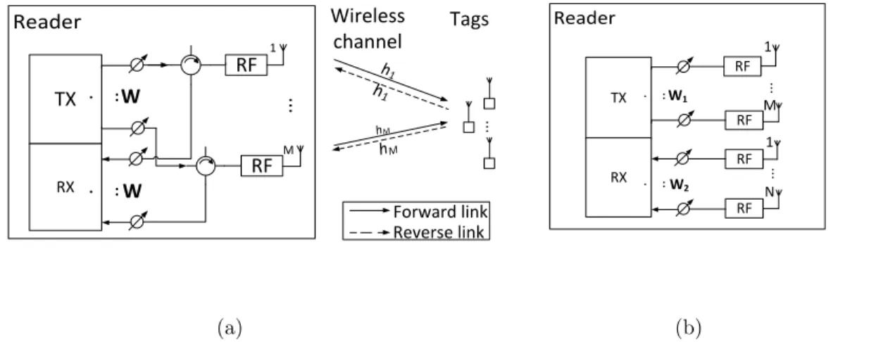
An RFID system mainly consists of a reader and a set of tags. The block diagram of the system is shown in Fig. 2.1(a), where M transmit/receive antennas are employed at the reader whereas each tag has a single antenna. In Fig. 2.1(a) the transmitter and receiver use a common set of antennas, which is referred to as a full-duplex reader, and the transmitter and receiver are connected via a circulator or a coupler [6]. On the other hand, if different sets of antennas are employed for transmitting and receiving, it is referred to as a half-duplex reader, shown in Fig 2.1(b).
For a full-duplex reader, we assume that the forward link and the corresponding reverse link observe the same channel coefficients (see Fig. 2.1(a)). On the other hand, for a half-duplex reader, forward and reverse links observe independent channel coefficients.
Reader TX RX RF RF .. . .. . ... ... W W 1 M h1 h1 hM hM Wireless channel Tags Forward link Reverse link (a) Reader TX RX RF RF .. . .. . ... W1 W2 1 M RF RF ... 1 N (b)
Figure 2.1: (a) A passive full-duplex multiple-antenna UHF RFID system and (b) a half-duplex reader.
Before analyzing the interrogation range of the multiple-antenna RFID system, we first consider the single-antenna case.
2.2.1
Single-antenna Case
We first consider the full-duplex case. At the very beginning, the reader transmits a continuous wave (CW) to power up the passive tag in the forward link. The received power by a tag can be written as
Ptag
RX (d) =PT XGrGtPL(d)|h|
2
, (2.1)
where PT X is the transmit power of the reader, Gr is the reader antenna gain, Gt is
the tag antenna gain, h is the channel coefficient, PL(d) is the path loss given by
PL(d) = λ 4πd 2 , (2.2)
whereλ is the wavelength of the carrier anddis the distance between the reader and the tag.
than the tag sensitivity PT S, i.e.,
PT XGrGtPL(d)|h|2 ≥PT S, (2.3)
which is the constraint of the forward link.
In the reverse link, after the tag is powered up, it scatters the signal back to the reader by modulating the received CW. The backscattered power received by the reader is given by PRXreader(d) = ηPtag RX (d)GrGtPL(d)|h| 2 = ηPT XG2rG 2 tP 2 L(d)|h| 4 , (2.4)
where η is the backscattering modulation efficiency of the tag.
In order to successfully demodulate the backscattered signal, the received backscat-tered power should be no less than the reader sensitivity PRS, i.e.,
ηPT XG2rG 2 tP 2 L(d)|h| 4 ≥ PRS, (2.5)
which is the constraint of the reverse link.
It is clear that both constraints (2.3) and (2.5) should be satisfied to determine the reader interrogation range d. From (2.3) and (2.5), we have
PL(d)≥ PT XGrGt|h|2 −1 PT S (2.6) and PL(d)≥pηPT XGrGt|h| 2−1p PRS. (2.7) Denote α, PT XGrGt|h|2 −1 PT S, β , √ ηPT XGrGt|h| 2−1√ PRS, and δ,α/β = (PT XPRS) −1 2 √ηP T S. (2.8)
If δ > 1, we have α > β, so once (2.6) is satisfied, (2.7) is always satisfied. In this case, the system is forward-link-limited (FLL) which means the interrogation range is the forward link range determined by (2.6). From δ >1 and (2.8), it can be easily derived that PT S >
p
η−1P
By substituting (2.2) into (2.6), we have (λ/4πd)2 ≥ PT XGrGt|h|2
−1
PT S, so it
follows that the maximum interrogation range is
dF LL = q (16π2P T S) −1 PT XGrGtλ2|h| 2 . (2.9)
If δ < 1, we have α < β. In this case, the system is reverse-link-limited (RLL) which means the interrogation range is determined by the reverse link range. From
δ <1 and (2.8), it can be easily derived thatPT S <
p
η−1P
T XPRS. The interrogation
range is determined by (2.7). By substituting (2.2) into (2.7), we have (λ/4πd)2 ≥ √
ηPT XGrGt|h|
2−1√
PRS, so it follows that the maximum interrogation range is
dRLL= r 16π2pP RS −1p ηPT XGrGtλ2|h| 2 . (2.10)
For half-duplex readers, the forward and reverse links observe different channel gains h1 and h2 respectively. The forward-link-limited and reverse-link-limited
max-imum interrogation ranges are
dF LL = q (16π2P T S) −1 PT XGrGtλ2|h1|2 (2.11) and dRLL = r 16π2pP RS −1p ηPT XGrGtλ2|h1| |h2|, (2.12)
respectively, under the assumption that the distance from the transmitter antenna to the tag and that from the tag to the receiver antenna are identical, which holds in practice when antennas are placed next to each other and the tag is relatively far from the antennas.
2.2.2
Multiple-antenna Case
Under full-duplex configuration, in the forward link, for the multiple-antenna case, the received power at the tag is given by
PRXtag(d) = PT XGrGtPL(d) wHh 2 , (2.13)
where h = [h1, . . . hM] T
is channel vector with hi being the channel coefficient from
the ith reader antenna to the tag antenna, M is the number of antennas, w = [w1, . . . , wM]
T
is the antenna weight vector, i.e., beamformer, withkwk= 1. Thus the constraint of the forward link with multiple-antenna configuration can be expressed as PT XGrGtPL(d) wHh 2 ≥PT S. (2.14)
In the reverse link, the received backscattered power at the reader is given by
PRXreader(d) = ηPtag RX (d)GrGtPL(d) wHh 2 = ηPT XG2rG 2 tP 2 L(d) wHh 4 . (2.15)
So we have the constraint of the reverse link for the multiple-antenna case as
ηPT XG2rG 2 tP 2 L(d) wHh 4 ≥PRS. (2.16)
Similar to the single-antenna case, we have that the system is forward-link-limited if PT S >
p
η−1P
T XPRS, with the corresponding maximum interrogation range
dF LLM A = q (16π2P T S) −1 PT XGrGtλ2|wHh|2. (2.17)
And the system is reverse-link-limited ifPT S <
p
η−1P
T XPRS, with the corresponding
maximum interrogation range
dRLLM A = r 16π2pP RS −1p ηPT XGrGtλ2|wHh|2. (2.18)
From (2.9), (2.10), (2.17), and (2.18), it can be derived that the interrogation range gain of the multiple-antenna case over the single-antenna case is |w
Hh|
|h| for both
FLL and RLL systems. Similarly, the maximum interrogation ranges for half-duplex systems are dF LLM A = q (16π2P T S) −1 PT XGrGtλ2|w1Hh1| 2 (2.19) and dRLLM A = r 16π2pP RS −p1 ηPT XGrGtλ2|w1Hh1| |wH2 h2| (2.20)
respectively, where w1 and w2 are antenna weights for the transmitter and receiver,
respectively.
The proper choice of the antenna weights w or (w1,w2) increases the
interro-gation range. There are several beamforming schemes in common use: equal-weight beamforming (EBF), random beamforming (RBF), and optimal beamforming (OBF). For EBF, the weight vectors are a normalized all-one vector i.e., w = w1 = w2 =
1
√
M[1,· · · ,1]
T where M is the number of antennas. For RBF, the weight vectors
are generated randomly following certain distribution and then normalized, e.g., ˜
w ∼ Nc(0,IM), w = w˜/kw˜k. Both EBF and RBF are simple to implement, but
their performances may be far from the optimum since they do not make use of the channel state information h or (h1,h2). On the other hand, the optimal
beamform-ers are channel-matched, i.e., the OBF is given by w = h/khk for full-duplex and w1 = h1/kh1k,w2 =h2/kh2k for half-duplex. Therefore, the OBF requires perfect
knowledge of the channel state which is unavailable at the reader at the startup of the system but is typically obtained by estimating the channel based on the reply signal from the tag. In other words, the tag must have been powered up before the reader is about to estimate the channel. In this sense, it is clear that there is no need to estimate the channel in order to improve the interrogation range since the tag has been powered up and the distance between the reader and tag has been physically determined. Moreover, introducing the channel estimation functionality will signif-icantly increase the complexity of the RFID system. In next section, we propose a blind adaptive beamforming (BABF) technique [36, 37] that exploits the channel state information but does not perform explicit channel estimation.
Algorithm 2.1 - Blind adaptive beamforming algorithm for full-duplex systems
1: Initializen= 0 andw(0) ∼ Nc(0,IM);
Repeat 2: n=n+ 1;
3: GenerateKp perturbation vectorspi∼ Nc(0,I), i= 1, . . . , Kp;
4: FormKp new weight vectors w˜i = w
(n−1)+βp i
kw(n−1)+βp
ik,i= 1, . . . , Kp;
5: Measure the received power PRX,ireader=ηPT XG2rG2tPL2
w˜Hi h 4 ,i= 1, . . . , Kp;
6: Updatew(n)=w˜I, whereI = arg max i P
reader RX,i ;
7: UntilPRXreader w(n)
−PRXreader w(n−1)< ε, whereεis the threshold.
2.3
Blind Adaptive Beamforming for RFID Reader
2.3.1
Full-duplex Reader
The goal for the BABF algorithm is to find the antenna weight vector that enables the reader to probe the tags at a given distance, and maximizes the received backscattered power from the tag. In full-duplex systems, the BABF scheme starts by sending the CW from the reader forprobing the tag, i.e., evaluating the backscattered power from the tag. At thenth iteration, given the weight vectorw(n−1),K
pperturbation vectors
pi are generated where pi ∼ Nc(0,IM), i= 1, . . . , Kp to form Kp new weight vectors
˜ wi ⇐ w(n−1)+βpi kw(n−1)+βp ik , i= 1, . . . , Kp (2.21)
where β is the weight adaptation step size. Then for each of these Kp generated
weight vectors, the corresponding received backscattered power (2.15) is measured at the reader. Finally, the weight vector is updated as the one that has the largest backscattered power among the Kp vectors in (2.21). The iteration terminates when
the received backscattered power fluctuates below a tolerance threshold. The algo-rithm is summarized as Alg. 2.1.
Algorithm 2.2 - Blind adaptive beamforming algorithm for M×N half-duplex systems
1: Initializen⇐0 andw(0)∼ Nc(0,IM+N);
Repeat 2: n=n+ 1;
3: GenerateKp perturbation vectorspi∼ Nc(0,IM+N),i= 1, . . . , Kp;
4: FormKp new weight vectors w˜i ⇐w(n−1)+βpi,i= 1, . . . , Kp;
5: Partition and normalize weight vectors: ˜ w1,i ⇐ kww˜˜i[1:M] i[1:M]k, w˜2,i⇐ ˜ wi[M+1:M+N] kw˜i[M+1:M+N]k, i= 1, . . . , Kp;
6: MeasurePRX,ireader=ηPT XG2rG2tPL2
w˜ H 1,ih1 2 w˜ H 2,ih2 2 ,i= 1, . . . , Kp;
7: Updatew(n)⇐[w˜1,I;w˜2,I], where I= arg max i P reader RX,i ; 8: UntilPRXreader w(n) −Preader RX w(n−1)
< ε, whereεis the threshold.
2.3.2
Half-duplex Reader
The BABF algorithm for half-duplex systems updates both w1 and w2
simultane-ously, and it is a variant of Alg. 2.1. Suppose that the half-duplex reader has M
transmit antennas and N receive antennas. Then we will use Alg. 2.1 to generate (M +N)-dimensional weight vectors, and break them into an M-dimensional trans-mit beamformer and an N-dimensional receive beamformer. At the nth iteration,
Kp new weight vectors are formed. The blind adaptive beamforming algorithm for
half-duplex systems is shown in Alg. 2.2.
Note that the BABF algorithm can not only extend the interrogation range, but also improve the ID data transmission reliability, which will be discussed in Chapter 2.4.
CW Query PC/XPC+EPC+CRC QueryRep ACK Reader Tag RN16 Select CW CW CW
Figure 2.2: Interactions between the reader and the tag.
2.4
Data Backscattering Transmission
After the tag has been powered up by the CW, the reader sends commands (e.g., Query) to communicate with the tag. The tag replies to the reader based on the backscattering modulation of the received CW. Fig. 2.2 illustrates the interaction between the reader and the replying tag during the inventory process. The Select command is used to select a tag population. An inventory process starts by the reader sending aQuery command to the tag, which broadcasts a frame consisting of F time slots. After receiving the Query command, each tag randomly selects a slot. The tag that picks the0th slot replies to the reader with RN16, which is a sequence of 16 bits randomly generated. Then, the reader decodes the received RN16, and sends the decoded 16 bits as the ACK to the tag. Next, the tag extracts the 16 bits from the ACK. If the extracted 16 bits are the same as the originally generated RN16, the tag then sends its ID, i.e., the electronic product code (EPC) to the reader. After receiving the ID of the current tag, the reader will send the QueryRep command to read the next tag. In this section, we assume that the process before the tag replying its EPC is perfectly done, and we focus on the EPC transmission performance of the tag. Note that the EPC is incorporated in a packet during the transmission and besides the EPC, the whole packet, which is 128-bit long, also includes protocol control / extended protocol control (PC/XPC) and cyclic redundancy check (CRC) [38]. In the following, PC/XPC+EPC+CRC is denoted as ID for simplicity. For simplicity, only the full-duplex system is considered in this section.
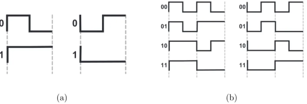
0 0 1 1 00 01 10 FM0 Symbols (a) 00 01 10 11 00 01 10 11 FM0 Sequences
Figure 6.9 – FM0 symbols and sequences
(b)
Figure 2.3: (a) FM0 symbols and (b) FM0 sequences.
scheme illustrated in Fig. 2.3. For FM0 encoding, there is always one phase inverse at every symbol boundary, and an extra phase inverse appears in the middle of symbol 0. Thus, the FM0 sequence is decoded by judging whether there is a phase inverse in the middle of each symbol.
2.4.1
Single-Antenna Case
Let r(ID)(t) denote the received complex baseband FM0 encoded ID signal by the
reader after passing through the direct-conversion receiver filter:
r(ID)(t) = hs(ID)(t) +nr(t), (2.22) where s(ID)(t) is the complex baseband FM0 encoded ID signal replied from the tag
and nr(t) is the complex Gaussian noise of the reverse link. Since the tag replies
the signal to the reader by modulating the received CW sent by the reader, in the baseband, s(ID)(t) could be expressed as
s(ID)(t) =√ηf(ID)(t) h+nf(t)
, (2.23)
wheref(ID)(t) is the FM0 encoded ID and nf(t) is the complex Gaussian noise of the forward link.
Suppose the timing synchronization is perfect and the sampling rate is T2. To decode the kth bit replied by the tag, the reader receiver performs the following
differential demodulation operation:
y(ID)(k) = Rer(ID)(kT +T /4)[r(ID)(kT + 3T /4)]∗ , (2.24) where Re{x}denotes the real part ofx, * is the conjugation operator,k is the symbol index, and T is the symbol duration of the backscattered signal.
Then the symbol a(k) is decoded according to the following:
ˆ a(k) = 1, if y(ID)(k)>0 0, if y(ID)(k)≤0 . (2.25)
2.4.2
Multiple-antenna Case
For the multiple-antenna case, (2.23) can be rewritten as
s(ID)(t) =√ηf(ID)(t) wHh+nf(t). (2.26) Thus, the received complex baseband signal at the ith antenna of the reader after passing through the filter is represented as
ri(ID)(t) =his(ID)(t) +nri(t), (2.27)
where nr
i(t) is the complex Gaussian noise at the ith antenna of the reverse link.
Similar to (2.24), for the multiple-antenna case, the receiver computes y(ID)(k)= Re (M X i=1 wir(iID) kT+T 4 wir(iID) kT+3T 4 ∗) = Re (M X i=1 |wi|2ri(ID) kT+T 4 ri(ID) kT+3T 4 ∗) , (2.28)
wherewidenotes the receive beamforming weight. Finally, the symbola(k) is decoded
according to (2.25).
We now consider the choice of the antenna weightwi. Although the OBF would be
the best choice, it requires channel estimation which is hard to implement under the current RFID standard. Therefore, the BABF algorithm can also improve the data
CW Select CW Query CW ACK CW QueryRep
RN16 PC/
XPC+EPC+CRC Reader
Tag BABF(Tag) BABF (Reader) Potential BABF (Tag) Potential BABF (Reader)
Figure 2.4: A MIMO RFID protocol with BABF algorithm.
transmission effectively as an approximation to the OBF weights. The beamformer vector w should be chosen to maximize the received SNR at the reader receiver, or equivalently, to maximize the received backscattered power (2.15) from the tag.
To this end, we need to point out that the BABF algorithm is a reader-tag in-teraction process that needs to be appended to the current RFID standard [38]. Specifically, the BABF algorithm should be executed before the Select command for tag activation and initial reading. In case that the channel state information changes during the communication with a tag, another round of weight updates can also be carried out before sending theQueryRep commands. A MIMO RFID protocol frame-work with the BABF algorithm that is compatible with the current RFID standard is shown in Fig. 2.4.
2.5
Tag Quantity Estimation
Upon interrogating the tags, the reader starts by broadcasting an initial frame con-sisting F time slots. Then each tag selects a slot at random from [0, F-1]. If more than one tag select the same slot, these tags will collide, so no tag could be read successfully. Since the number of tags to be identified is unknown to the reader in the initial interrogation round, if the issued frame size (i.e., the total number of slots) is much larger than the tag quantity, more slots of the frame will be empty which wastes the limited channel resource and decreases the system throughput; if the frame size
−15 −10 −5 0 5 10 15 −15 −10 −5 0 5 10 15 Quadrature In−Phase (a) −15 −10 −5 0 5 10 15 −15 −10 −5 0 5 10 15 Quadrature In−Phase (b)
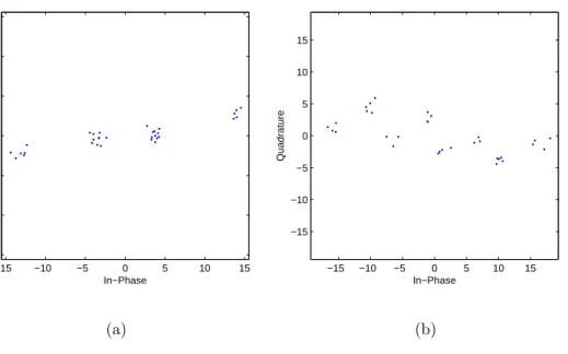
Figure 2.5: RCS plots based on the reception of the replied RN16s of tags: (a) two tags replying simultaneously resulting in four clusters and (b) three tags replying simultaneously resulting in eight clusters.
is much smaller than the tag quantity, more collisions will occur which also decreases the system throughput. It is known that the system achieves the optimal throughput when the assigned frame size equals to the number of tags in the interrogation range. A number of works have addressed the estimation of the tag quantity. A collision ratio estimation (CRE) algorithm is proposed in [34] by searching the number of tags to make the actual collision ratio equal to the expected one. Three Bayesian methods are proposed in [35] to estimate the tag quantity with reduced complexity. In [22] the number of tags in a collision slot is estimated according to the tag’s radar cross-section (RCS) plot.
After the initial interrogation round, the reader may experience three kinds of time slots: empty slot where there is no tag replying, single-tag slot where there is only one tag replying, and collision slot where there are more than one tag replying simultaneously. Since those unsuccessfully read tags due to the erroneous transmission in the single-tag slot or due to the collision in the collision slot will participate in
the next interrogation round, if the number of those unsuccessfully-read tags in the current frame could be estimated, the frame size of the next interrogation round could be determined according to the estimation result so as to maximize the system throughput. Suppose that the current frame containsN unsuccessfully-read slots due to the erroneous transmission or the collision. At each slot, the reader estimates the number of tags replying, say ni for the ith slot. Then the total number of the tags
participating in the next interrogation round could be estimated asn1+. . .+nN, and
the frame size of the next interrogation round could be set accordingly. For simplicity we consider only full-duplex systems.
In the following, we assume that the reader knows there is one tag in each unsuccessfully-read single-tag slot and we focus on the estimation of the number of tags in each collision slot based on the collided signal.
Instead of the tag ID, it is a sequence of FM0 encoded random 16 bits (RN16) that is firstly replied to the reader by the tag upon receiving the Query command. The reader should be able to successfully receive and decode this sequence to enable the subsequent communication. But if collision happens, which means multiple RN16s from different tags are sent to the reader simultaneously, the reader is unable to decode the received overlapped RN16s. Thus the collided tags cannot be read successfully and will reply in the next available interrogation round.
It is noticed that one tag’s response RN16 signal contributes two clusters in the RCS plot [22], and R simultaneously replying tags produce 2R clusters in the plot ideally, as illustrated in Fig. 2.5, where the sampling rate is two samples per bit. Consequently, if the reader is able to estimate the number of clusters, the number of the collided tags can be easily derived. Based on this idea, we next develop a tag quantity estimator.
2.5.1
Single-antenna Case
In this subsection, we propose a clustering algorithm to estimate the number of tags involved in the collision slots. We focus on the single receive antenna case first. The clustering algorithm is described as follows.
We consider a specific collision slot. Letr(RN16)(t) denote the received overlapped
complex baseband RN16 signal in this slot after passing through the filter, which can be expressed as r(RN16)(t) = Ntag X n=1 hns(nRN16)(t) +n r(t), (2.29)
whereNtag ≥2 is the number of tags replying in the slot, hn is the channel coefficient
from the nth tag to the reader ands(nRN16)(t) is the replied RN16 signal from thenth
tag, which is given as
sn(RN16)(t) =√ηfn(RN16)(t) hn+nf(t)
, (2.30)
where fn(RN16)(t) is the FM0 encoded RN16 generated by thenth tag.
Suppose the timing synchronization is perfect and the sampling rate is T2 at the reader receiver. Then the received signal sample set in this collision slot is
S = r(RN16) 2k+ 1 4 T , k = 0, ...,31 . (2.31)
After obtaining S, the reader starts clustering the samples by first selecting one element in S at random. Then the distances between the selected element and all other elements are calculated. Those elements with distances from the selected ele-ment being no larger than r form a cluster together with the selected element, where
r = ρσ and ρ is a parameter. Next, the reader repeats the above clustering steps for the elements which have not been clustered until all elements in S are clustered. Finally, the number of tags in this slot can be derived by counting the number of clusters Nc inS. The proposed tag quantity estimator is summerized in Alg. 2.3.
Algorithm 2.3 - Tag quantity estimation algorithm
1: Forj = 1, ..., Mcs, where Mcs is the number of collision slots in the current frame;
2: Nc= 0;
3: ObtainS according to (2.31) in thejth slot;
4: WhileS is not empty,DO:
5: Randomly pick one element sk∈ S;
6: Calculatedh =|sk−sh|, whereh= 1, ...,|S|;
7: Choose elements {sg :dg ≤ρσ} to form a cluster and remove them fromS;
8: Nc=Nc+ 1;
End While
9: Estimate the number of tags in the jth collision slot as dlog2Nce;
End For
2.5.2
Multiple-antenna Case
Although the reader could observe 2R clusters with R tags involved in a collision slot ideally, it is possible that the actual number of observed clusters is less than 2R.
The reason is that the clusters may overlap with each other due to the impact of channel and noise. For example, the reader may observe only four clusters due to the overlapping effect, albeit there are three tags replying simultaneously and 23 = 8 clusters are supposed to be observed ideally.
Multiple receive antennas may help overcome the overlapping effect. Suppos-ing that multiple antennas are spatially well separated, while one antenna observes overlapped and indistinguishable clusters, other antennas may observe well-separated clusters.
For the multiple-antenna case, (2.30) can be rewritten as
s(nRN16)(t) =√ηfn(RN16)(t) wHhn+nf(t)
, (2.32)
from the ith reader antenna to thenth tag. And (2.29) now becomes ri(RN16)(t) = Ntag X n=1 hins(nRN16)(t) +n r i(t), (2.33)
which is the received overlapped complex baseband RN16 signal in a collision slot from the ith receive antenna after passing through the filter. Stacking the received RN16 signals (2.33) of each antenna, we have the vector
r(RN16)(t) = Hs(RN16)(t) +nr(t), (2.34) wherer(RN16)(t) = [r(RN16) 1 (t), ..., r (RN16) M (t)]T,s(RN16)(t) = [s (RN16) 1 (t), ..., s (RN16) Ntag (t)] T, nr(t) = [nr1(t), ..., nrM(t)]T, and H= h11 · · · h1Ntag .. . . .. ... hM1 · · · hM Ntag . (2.35)
Then, the signal sample set in (2.31) becomes
S = r(RN16) 2k+ 1 4 T , k = 0, ...,31 . (2.36)
The clustering algorithm is similar to Alg. 2.3, except that it is now applied to the vector samples in (2.36) and the corresponding distances between vectors are used.
2.6
Simulation Results
In this section, simulation results are presented. The system parameters are set as follows. Carrier frequency fc = 915 MHz, the total transmit power PT X = 1W (30
dBm), reader antenna gainGr= 2 dBi, tag antenna gainGt= 0 dBi, reader sensitivity
PRS = 3.16×10⁻⁸ mW (-75 dBm), modulation efficiencyη = 0.25, weight adaptation
step sizeβ = 0.05, the number of tags in the reader interrogation range is uniformly distributed in [50, 500] and the initial frame size Finit = 256. Finally, the Rician
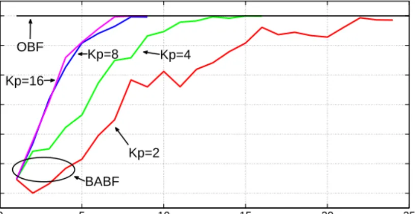
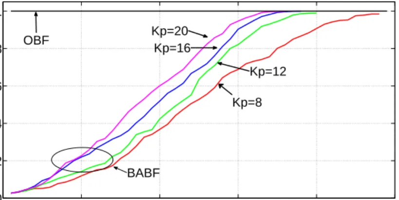
0 5 10 15 20 25 0.4 0.5 0.6 0.7 0.8 0.9 1 Iteration Number Normalized Power |w H h| 4 OBF Kp=16 Kp=8 Kp=4 Kp=2 BABF
Figure 2.6: The convergence of the proposed BABF algorithm with different values of Kp in full-duplex setting, M = 2.
2.6.1
Interrogation Range Performance
We first illustrate the convergence of the proposed BABF algorithm. Fig. 2.6 shows the received power metric wHh
4
as in (2.15) versus the iteration number in one simulation for a full-duplex system with the number of antennas M = 2. The perfor-mance of OBF with ideal CSI is also plotted as a benchmark. It can be observed that the performance of the proposed BABF approaches that of OBF, and the convergence rate increases with the number of perturbationsKp. A similar plot for the half-duplex
system with M =N = 2 is given in Fig. 2.7. In this setting, the number of antenna weights that need to be optimized doubles, so a larger Kp and more iterations are
needed to achieve the benchmark OBF performance.
The tag sensitivity varies from tag to tag. In the following simulations, we fix the reader sensitivity and vary the tags with different sensitivities. Assume there is only one tag in in each round of interrogation range simulation.
2.6.1.1 Interrogation Range for Full-duplex Systems
For full-duplex systems, we choose the tag sensitivity PT S = 0.04 mW (-14 dBm)
so that PT S >
p
η−1P
0 10 20 30 40 50 0 0.2 0.4 0.6 0.8 1 Iteration Number Normalized Power |w H h| 4 OBF Kp=20 Kp=16 BABF Kp=12 Kp=8
Figure 2.7: The convergence of the proposed BABF algorithm with different values of Kp in half-duplex setting, M =N = 2.
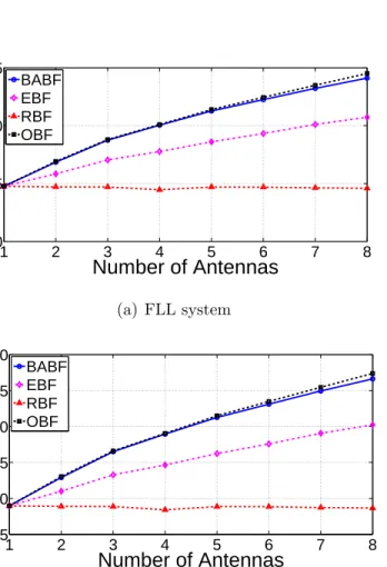
interrogation range versus the number of antennas under this setup. Although only BABF, EBF and RBF can be employed in practice as they do not require the channel state information, as a performance upper bound, we also present OBF performance assuming the reader has the channel state information at the startup of the system. It can be observed that OBF is able to read at the longest distances. While the interrogation range generally increases with the number of antennas, the reader with BABF has the closest performance to that of OBF among others. Specifically, the interrogation range is increased from 4.76 m (M = 1) to 6.84 m (M = 2), then to 10.05 m (M = 4) and to 14.11 m (M = 8) for BABF; and for EBF, the interrogation range is increased from 4.76 m (M = 1) to 5.83 m (M = 2), then to 7.76 m (M = 4) and to 10.73 m (M = 8). Interestingly, unlike other beamforming schemes, for RBF the average interrogation range decreases slightly as the number of antennas increases.
Next, we choose the tag sensitivity PT S = 0.01 mW (-20 dBm) so that PT S <
p
η−1P
T XPRS and the system is RLL. Fig. 2.8(b) shows the average interrogation
range versus the number of antennas under this setup. We observe similar range improvements as in FLL systems. Moreover, under the same antenna configuration,
1 2 3 4 5 6 7 8 0 5 10 15 Number of Antennas Average Range (m) BABF EBF RBF OBF (a) FLL system 1 2 3 4 5 6 7 8 5 10 15 20 25 30 Number of Antennas Average Range (m) BABF EBF RBF OBF (b) RLL system
Figure 2.8: Average interrogation range versus number of antennas under full-duplex setting.
the interrogation range of the RLL system is larger than that of the FLL system. This is due to the improvement of the tag sensitivity in RLL systems, which enables the tags to detect weaker signals.
2.6.1.2 Interrogation Range for Half-duplex Systems
In the half-duplex setting, the channel state information at the transmitter and re-ceiver is not balanced, and the power transfer efficiency is not equivalent for the forward link and reverse link. Therefore, using tags with 0.01 mW tag sensitivity does not simply imply that the system is absolute RLL anymore. In this case, though for most of the time the system is still RLL, there is a small portion of instances that it is FLL. It is the same case for tags with 0.04 mW sensitivity. Hence, we continue using 0.04 mW and 0.01 mW tag sensitivities in the simulation, but the results are not classified as FLL and RLL here.
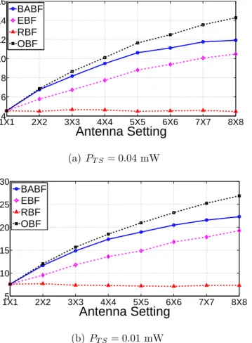
We observe similar pattern in the average interrogation range plot shown in Fig. 2.9 for symmetric half-duplex systems, which means the numbers of transmit and receive antennas are the same. For the OBF scheme, the average ranges of half-duplex readers are close to those of full-half-duplex readers. The average ranges for the BABF scheme are not as long as those in full-duplex configuration, but they are still much better than EBF. Finally, RBF does not show interrogation range improvement as the number of antennas grows for the half-duplex setting as well.
Table 2.1 presents the numerical results for half-duplex readers with asymmetric settings. In all antenna settings, BABF has the best performance in interrogation range as expected. One feature that can be drawn from this table is that when the total number of antennas are fixed, readers with more antennas on the transmitter outperform readers with more antennas on the receiver. For instance the 2×1 and 3×2 settings in Table 2.1, all the beamforming schemes have longer reading distances than those in the 1×2 and 2×3 settings.
1X14 2X2 3X3 4X4 5X5 6X6 7X7 8X8 6 8 10 12 14 16 Antenna Setting Average Range (m) BABF EBF RBF OBF (a)PT S = 0.04 mW 1X15 2X2 3X3 4X4 5X5 6X6 7X7 8X8 10 15 20 25 30 Antenna Setting Average Range (m) BABF EBF RBF OBF (b) PT S = 0.01 mW
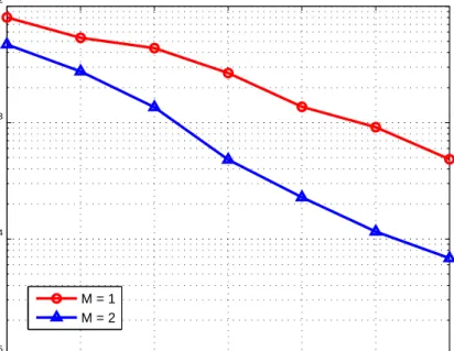
Figure 2.9: Average interrogation range versus number of antennas under half-duplex setting. 0 5 10 15 20 25 30 35 40 6 7 8 9 10 Velocity (m/s) Average Range (m) 4 Antennas BABF 2 Antennas BABF
Table 2.1: Average interrogation range for different numbers of antennas and BF schemes in half-duplex systems.
Antenna setting BF scheme Tag sensitivity 0.04 mW 0.01 mW 1×2 OBF 4.6541 8.9858 BABF 4.6528 8.9487 EBF 3.7925 7.6469 RBF 4.5888 7.6469 2×1 OBF 6.8128 9.9277 BABF 6.7124 9.7842 EBF 6.5830 8.8297 RBF 4.6682 7.5358 2×3 OBF 7.1437 12.9182 BABF 6.9281 12.5044 EBF 5.3290 9.3442 RBF 4.6033 7.4134 3×2 OBF 8.6924 14.1891 BABF 8.3997 13.6904 EBF 7.4709 11.3799 RBF 4.4826 7.6450
RFID reader system with BABF shows stable result as well. Fig. 2.10 presents the average interrogation range as a function of the velocity of the reader for a 2-antenna and a 4-antenna system. PT S = 0.04 mW is considered for both systems. It is
observed that the range declines when the velocity increases, but the interrogation range can always be maintained and more than 90% of the reading range in the stationary environment can be achieved. The range reduction of the 4-antenna reader is greater than that of the 2-antenna system, which can be explained by the fact that every antenna link is slow varying, and therefore the total channel variation is stronger for the 4-antenna system. In practice, considering a scenario that the RFID reader is carried by a technician and makes readings with walking speed, the interrogation range is almost constant according to Fig. 2.10.
2.6.2
Data Transmission Performance
Once a tag successfully receives theACK command sent by the reader, it will reply to the reader using a 128-bit packet that includes PC/XPC, EPC, and CRC. If the packet is not received successfully by the reader, the tag will then enter the arbitration state to wait for replying to the reader in the next interrogation round. In this subsection, instead of the bit error rate (BER) performance (e.g., [12] [13]), the more appropriate packet error rate (PER) performance of the system is evaluated and the performance gain of employing multiple antennas is examined.
Fig. 2.11 shows the PER performance versus the transmit signal-to-noise ratio (SNR) for data transmission. For BABF, we setKp = 8 and the number of iterations
is 30. It can be observed that the PER performance is significantly improved as the number of antennas M increases. With M = 2, BABF has better PER performance than RBF and EBF. The performance offered by BABF is very close to the optimum, i.e., OBF with perfect CSI. One can also observe that the proposed BABF scheme offers about 21 dB gain over the single-antenna case at the PER of 10−2 with M = 2
5 10 15 20 25 30 35 40 45 50 55 10−4 10−3 10−2 10−1 100 SNR (dB) PER M=1 RBF EBF BABF
OBF w/ perfect CSI M=2
Figure 2.11: PER performance in a Rician fading channel (K = 2.8 dB) for different BF schemes.
10 15 20 25 30 35 40 10−5 10−4 10−3 10−2 SNR (dB) Normalized MSE M = 1 M = 2
Figure 2.12: Normalized MSE of the estimated number of tags versus SNR.
2.6.3
Tag Quantity Estimation Performance
We suppose that the reader has the knowledge of the noise varianceσ2 and the collided
tags have the same distance from the reader. In Alg. 2.3, ρ should be specified in advance. We resort to simulations to find the optimal value of ρ by making 5000 simulation runs to evaluate the performance for eachρvalue in the interval of [1.5,5.5] with step size 0.1.
Fig. 2.12 shows the normalized MSE of the estimation versus SNR. It is seen that the multiple-antenna configuration (M = 2) leads to much more accurate estimation than the single-antenna one.
2.7
Experimental Validation
To evaluate the performance of the multiple-antenna RFID system, a number of exper-iments have been carried out. The goal of these experexper-iments is to show the readability
of the different beamforming schemes at various interrogation ranges, and compare it with that of the single antenna system. Since commercially available RFID readers do not support MIMO or beamforming functionality, a 2×1 half-duplex reader prototype is built using the Universal Software Radio Peripheral (USRP) with SBX daughter-boards. The setup has a wide bandwidth that cover 400 to 4400 MHz, and it can provide up to 100 mW of output power. This prototype consists of three S9028PCR circular polarity panel antennas by Larid Technologies : two for transmitting, and one for receiving. The antennad have a gain of 8 dBic. Each antenna is connected to an Ettus Research USRP N210. All the USRPs are connected to a computer, and LabView 2014 is the software used to control and interface. The reader operates at carrier frequency of 915 MHz, IQ rate of 1 MHz, and LabView program gain of 17. The RFID tag tested in this experiment is a UPM Raflatac FROG tag. Note that all the measurements in our experiments should be collected from the tag responses to the EPC commands in the current EPC standard [38], which is the only protocol the commercial tag complies with. In our case, Query commands are transmitted, then the RN16 responses are recorded as measurements.
The experiments are set up in a lab environment shown in Fig. 2.13. In order to compare the different beamforming schemes together with the single antenna reader, the tag is read at a series of distances, and its responses are recorded at each position. Specifically, eight evenly spaced points are selected along the center line illustrated in Fig. 2.14. The tag is placed and pointed horizontally to the antennas with a line of sight path in between.
In real RFID readings it takes at least a timeout interval [38] to judge if the tag has been activated. Hence it is not practical to find the exact maximum interrogation range within limited time like in Fig. 2.9. The power received by the tag is also largely affected by the channel state which varies from rounds to rounds. Therefore, in this experiment a large number of readings are tested at each marked location in Fig. 2.14. For each setting, the number of the RN16 tag responses and the total number
Figure 2.13: Experiment setup. R ec ei vi n g A n tt en n a Tran sm it ti n g A n te n n a 2 Tr an sm it ti n g A n te n n a 1 1 2 c m 120 cm 30 cm 30 cm 30 cm 30 cm 30 cm 30 cm 30 cm Tag Position 1 2 3 4 5 6 7 8
1 2 3 4 5 6 7 8 0 0.2 0.4 0.6 0.8 1 Tag Position Probability BABF RBF EBF SA1 SA2
Figure 2.15: Probability of successful RFID tag reading.
of reader Query attempts are counted. Thus instead of the average interrogation range in Chapter 2.6, the percentages of successfulQuery-RN16 interaction calculated from the collected data are compared among all the beamforming settings. The tag’s backscattered signal strength is also measured in the experiments. It is clear that higher percentage of successful reading indicates better beamforming scheme is at a given position, and so does the stronger signal strength. Therefore, in the experiment we use both the percentage and the signal strength as measures of reader performance. Fig. 2.15 shows the probabilities of successful RFID tag reading with the different beamforming schemes at selected positions. Obviously, BABF has the largest and most consistent chance to read a tag at all positions. It guarantees successful tag reading at the first 6 points (270 cm), and maintains high probability (0.9 and 0.7) to read the tag at longer distances. Readers with EBF and RBF have similar probability performance; the EBF curve is slightly higher than that of RBF. For these two beam-forming settings, neither of these tag positions has zero readings or guarantee perfect readings. Contrast to EBF and RBF, the single-antenna settings (transmitting with either antenna 1 or antenna 2) almost ensure reading when the tag is relatively close to the antenna. However, single antenna readers almost miss all the readings at dis-tances farther than the 3rd point (180 cm). This result illustrates that RFID reader
1 2 3 4 5 6 7 8 0 0.01 0.02 0.03 0.04 0.05 Tag Position Amplitude BABF SA1 SA2 EBF RBF
Figure 2.16: Backscattered signal strength received
with single antenna is less sensitive to the channel state, but long distance readings require MIMO settings. For all these antenna settings the probability of successful reading decreases as the tag moves away from the antennas. This trend matches with the simulation results as well. It is interesting that the probabilities for the readers at the 5th point (240 cm) using EBF, RBF and single-antenna 2 are slightly higher than those at the 4th point, which act against the overall trend. This may be caused by environmental factors, e.g., the electromagnetic wave reflection in the laboratory amplifies the signal reception at the 5th point. Nevertheless, the results clearly show that the multiple-antenna RFID reader is more reliable at long distances, and in par-ticular the proposed blind adaptive beamforming algorithm leads the tag reading rate at all distances.
Fig. 2.16 is the plot of backscattered signal amplitude received by the reader. Similar to the probability plot, the reader receives the strongest signal response from the tag when it employs BABF. Readers using EBF and RBF generally can obtain stronger signal at long distances, but have close readings to single antenna reader in short range.
From both the probability and signal strength plots, it is seen that the MIMO RFID reader exhibits a clear advantage in long range interrogation compared with the
standard single-antenna readers. Moreover, the BABF algorithm is validated as an effective and stable technique to find the near-optimal antenna weights, and enhance the reader performance at all distances. Note that the difference of interogation range values in the experiment and the simulation is mainly caused by the difference of transmit power in each case. However, RFID systems with multiple antennas always outperform the single antenna systems in both cases.
2.8
Conclusions
We have proposed a passive multiple-antenna UHF RFID system with the reader equipped with multiple antennas and each tag equipped with a single antenna. The reader interrogation range, data transmission performance and the estimation of tag quantity have been investigated. In particular, the proposed BABF algorithm is performed to optimize the beamforming weights of the reader. As shown in Fig. 2.4, the improvement of the interrogation range is achieved during the transmission of CW before theSelect command is sent for the FLL system and during the backscattering transmission of the tag for the RLL system.
Our results indicate that under the multiple-antenna configuration, especially with the BABF scheme, the interrogation range extends substantially. The PER perfor-mance of the data transmission approaches the optimal beamforming perforperfor-mance with BABF algorithm as well without channel estimation. Finally, we note that the proposed MIMO RFID reader with blind adaptive beamforming complies with the current RFID standard and hence they can be readily implemented in existing systems.