University of Connecticut
University of Connecticut
OpenCommons@UConn
OpenCommons@UConn
Honors Scholar Theses
Honors Scholar Program
Spring 5-27-2020
Evaluating Driving Performance of a Novel Behavior Planning
Evaluating Driving Performance of a Novel Behavior Planning
Model on Connected Autonomous Vehicles
Model on Connected Autonomous Vehicles
Keyur Shah
Follow this and additional works at: https://opencommons.uconn.edu/srhonors_theses
Part of the Artificial Intelligence and Robotics Commons, Computational Engineering Commons, Controls and Control Theory Commons, Control Theory Commons, Digital Communications and Networking Commons, Navigation, Guidance, Control, and Dynamics Commons, Systems and Communications Commons, and the Theory and Algorithms Commons
Recommended Citation
Recommended Citation
Shah, Keyur, "Evaluating Driving Performance of a Novel Behavior Planning Model on Connected Autonomous Vehicles" (2020). Honors Scholar Theses. 684.
Evaluating Driving Performance of a
Novel Behavior Planning Model on
Connected Autonomous Vehicles
Keyur Shah
Thesis Advisor: Dr. Fei Miao
Honors Advisor: Dr. Zhijie Shi
Abstract
Many current algorithms and approaches in autonomous driving attempt to solve the “trajectory generation” or “trajectory following” problems: given a target behavior (e.g. stay in the current lane at the speed limit or change lane), what trajectory should the vehicle follow, and what inputs should the driving agent apply to the throttle and brake to achieve this trajectory? In this work, we instead focus on the “behavior planning” problem—specifically, should an autonomous vehicle change lane or keep lane given the current state of the system?
In addition, current theory mainly focuses on single-vehicle systems, where vehicles do not communicate with their surroundings. However, other works have showed opportunities for data sharing between vehicles and other vehicles (V2V) or road infrastructure (V2I) to improve driving algorithms. For example, a vehicle’s lane changing decisions on a highway might be improved by using traffic density data from other cars further ahead, beyond the first vehicle’s own field of vision.
In this work, we use the CARLA vehicle simulator to implement a simple behavior planning algorithm inspired by previous work from collaborators at UConn. The algorithm uses shared V2V information about position and velocity of nearby neighbors to improve lane changing decisions while still maintaining vehicle safety. We observe the driving performance of the fleet of connected vehicles under various traffic conditions, focusing on speed and passenger driving comfort.
The goals of this project are to demonstrate the performance improvements that result from V2V information sharing, highlight safety challenges and solu-tions during lane-changing, and lay the groundwork to develop other behavior planning algorithms in the future. Our lab plans to use this work to continue future autonomous driving research.
1
Introduction
1.1
Autonomous Vehicle Development
The development of autonomous vehicle driving algorithms has been a hot area of study and captured the public imagination in recent years. Car manufac-turers and technology companies alike have been racing to deploy vehicles that exhibit increasingly higher levels of autonomy. In 2016 it was estimated that the automotive industry spent aboute77 Billion worldwide on innovation and R&D [1], and the race to develop driverless cars continues to be a top priority for these companies today. The payoff is obvious: A road full of self-driving vehicles has the potential to prevent accidents, improve congestion, reduce energy con-sumption and pollution, increase productivity, and improve accessibility. These massive potential rewards have led to significant interest from governments and the public sector as well—one famous example is the DARPA Challenge funded by the US Department of Defense.
Despite the amount of interest in the field, autonomous vehicle technol-ogy still faces many challenges on the road to these goals. Autonomous vehicles must be able to share the road with sometimes-unpredictable humans, and make choices based on incomplete information. Although the decision-making process is messy, it can be made significantly easier by providing the driving agent with more data. Camera, lidar, and GPS data are common inputs to driving algo-rithms that can increase driving performance by giving the autonomous vehicle more information about its surroundings. Our lab, the Miao group1at the Uni-versity of Connecticut, is conducting research on inter-vehicle communication as another way for the autonomous driving agent to gather more knowledge.
1.2
Connected Autonomous Vehicle Behavior Planning
In this paper, I focus on developing a driving algorithm for Connected Au-tonomous Vehicles (CAVs), which share data with other entities on the road. Although much of the current autonomous vehicle research centers around sce-narios with many independently-controlled vehicles, significant potential exists for vehicles to use data from other participants on the road to improve their con-trol decisions [2]. Vehicle-to-Vehicle (V2V) and Vehicle-to-Infrastructure (V2I) communication are now possible using existing communication technology, en-abling this new level of vehicle connectedness [3]. However, existing control approaches for CAVs have largely focused on the problem of driving in a cer-tain lane at a cercer-tain speed, assuming that the lane and speed have already been decided. [2] cites Adaptive Cruise Control [4], and Cooperative Adaptive Cruise Control [5] as relevant examples that don’t address the “behavior plan-ning” question. Specifically, in this work I divide autonomous vehicle control into three layers:
1. Behavior Planning, in which the vehicle sets high-level “goals” such as keeping or changing lanes
2. Path Planning, where the vehicle charts an ideal course to follow based on the selected behavior
3. Vehicle Control (or Path Following), in which the vehicle uses a control loop to follow its planned trajectory
This three-layer division of control is a standard framework used for au-tonomous driving and many other applications in robotics [6]. Good vehicle control approaches have been known for a while (Model-Predictive Control, Control Lyapunov, etc.) [7][8], and path planning is often done by simply try-ing to track the center line of a lane. However, behavior planntry-ing currently has great potential for improvement, especially in situations with multiple con-nected vehicles. Exchanging information with other neighbors can allow a ve-hicle’s knowledge about the road to extend further than its own field of vision. This work will focus on the implementation of a proposed behavior planning algorithm for connected autonomous vehicles.
1.3
Project Goals
This Honors Thesis project was inspired by the behavior planning algorithm proposed in [2]. Using a hybrid system model, it models the behavior of the system in a discrete state space, and the physical state of the vehicle in a continuous space. While I keep the same three discrete states, (Lane Keeping, Change Left, Change Right), I propose new discrete state transition functions that require less shared information. My proposed switching functions also give a specific safety procedure designed for PID control, which is not considered in [2]. The goal of my project is threefold:
• First, to propose a novel behavior-planning algorithm which outperforms a baseline in a realistic (simulated) environment
• Second, to evaluate driving performance of a fleet of CAVs running the algorithm in various conditions
• Third, to create a general platform for future CAV behavior planning research by our lab
The rest of this paper shall be organized as follows: In Section 2, I give a precise mathematical definition of a shared-information lane changing algorithm. In Section 3, I discuss how I tested the algorithm and what results were obtained. Finally, in Section 4, I offer some concluding remarks.
2
Behavior-Planning Algorithm
This work specifically addresses the situation of several connected autonomous vehicles driving on a multi-lane highway (which may include some non-connected vehicles as well). Here I assume that a suitable V2V communication system exists with negligible communication loss or delay, and that all transmitted information can be regarded as true. Future work may address how to make the algorithm resilient to missing or faulty data.
2.1
Hybrid System Vehicle Model
Like in the preceding work [2], I model the vehicle as a Hybrid System with Controllable Switching (HSCS). In this model, an ego vehicle has discrete states which represent its lane-change behavior (e.g. lane changing or keeping) and continuous states which capture its position, velocity, and other physical at-tributes.
Definition 2.1 (Hybrid System with Controllable Switching). A HSCS is a collectionH = (Q, X, U,Init, Inv, f, G, δ) where:
• Q={q0, q1, . . . , qn}is a finite set of discrete states.
• X ⊆RN is a compact set of continuous states.
• U ⊆RM is a compact set of the control inputs in continuous space.
• Init⊆Q×X is the set of initial states.
• Inv:Q→X assigns to eachqan invariant set;
• f :Q×U×X →X assigns to eachq∈Qa continuous vector fieldf(·, q), a function fromX×U toX.
• Gq→q0 :Q×Q→X assigns each (q, q0) a guard. A transition from state
qto stateq0 is triggered when the continuous state is withinGq→q0.
• δ: X×Q→Qis a switching controller satisfying the following form:
q(t+) =δ(q(t), x(t)), andx(t+) =x(t),
where the switching controllerδ assigns a hybrid system (q(t), x(t)) into a new discrete stateq(t+) whenx(t)∈Gq(t)→q(t+).
In this model, the discrete state space Q represents the lane-changing be-havior. The continuous state spaceX captures both the vehicle’s own physical state variables (position, velocity, ...) and shared information (knowledge about other neighbors’ state variables). Urefers to the vehicle’s driving control inputs.
2.2
Vehicle-to-Vehicle Communication
Definition 2.2 (-leader). Vehiclej=6 iis an-leader of vehicleion lanekif:
kri(t)−rj(t)k ≤,j is ahead of i, andj is on lanek
whereri(t) represents the position vector of vehicleiat time instantt. Also let
L(i, k, t) ={j6=i:j is an-leader ofion lane k}
At each timestep, vehicles will receive information about current position, velocity, and lane number (1,2, ...) from each of their-leaders on their own lane and the adjacent lanes. Although position could be inferred by a vehicle with a camera or lidar sensor (and velocity could be too, by taking derivative across several sensor readings), sharing position and velocity over a network may give more accurate readings and allow the ego vehicle to receive data from vehicles that are hidden from its direct field of view (e.g. by a curve, another vehicle, etc).
L is the basis of the algorithm’s intelligent lane changing decisions. In this
work, I do not consider the problem of how to select good , but assume that some reasonably large has been chosen which still satisfies the no-loss and no-delay conditions.
2.3
Collision Avoidance
While connected vehicles receive precise information about position, velocity, and lane from their-leaders, they must also have some basic knowledge about the unconnected vehicles on the road: specifically, they must be able to avoid an imminent collision with any vehicle. To maintain safety while driving, each vehicle maintains three hazard sets:
Definition 2.3(Current lane hazardsHc(i, t)). While traveling on the current
lane, we are only worried about colliding with a vehicle in front of us:
Hc(i, t) ={j=6 i:kri(t)−rj(t)k ≤Θc,j is ahead ofioni’s lane}
Definition 2.4 (Left and right hazards Hl(i, t), Hr(i, t)). When making a
change, we are worried about cars anywhere near us in the adjacent lane:
Hl(i, t) ={j6=i:kri(t)−rj(t)k ≤Θl andj is oni’s left lane}
Hr(i, t) ={j6=i:kri(t)−rj(t)k ≤Θr andj is oni’s right lane}
To detect other nearby vehicles, I assume that all autonomous vehicle on the road are equipped with a camera, lidar, or other similar object detection sensor. The algorithm does not use the contents of these sets – it only checks if they are empty or nonempty. Because of this, a camera or lidar can be used to check the presence of any objects in the hazard regions, whereas detecting-leaders potentially requires the ego vehicle to see hidden vehicles beyond its field of
vision (and must therefore be done over the V2V network). Along with other vehicles, the hazard sets should also include any other non-vehicle obstructions on the road.
Figure 1: Illustration of hazard and information sharing distances on a three lane road. The road may contain an assortment of connected vehicles (red) and unconnected vehicles (gray).
2.4
Discrete States
I model lane changing with the following three discrete states:
• Lane Keeping (LK): Vehicles are initialized with a starting state of
LK. In this state, a vehicle travels on a lane with a given target speed (which it may or may not actually be traveling at), while always satisfying certain safety constraints (such as not coming too close to the vehicle in front).
• Change Left (CL) / Change Right (CR): The vehicle attempts to move left or right to the adjacent lane if possible. The vehicle must still satisfy safety requirements in both its current lane and the lane it is chang-ing into until the change is complete. Once completed or aborted, the vehicle’s discrete state returns toLK.
The system can only transition betweenLK and one of theCL/CR states. No transition exists fromCLdirectly toCR, or vice versa.
2.5
Continuous Vehicle States and Control Inputs
Many controllers represent a vehicle at timetwith a simple state vectorX(t) = [x(t), y(t), ψ(t), v(t)] where (x(t), y(t)) are the coordinates of the vehicle’s center of mass,ψ(t) is the heading angle (yaw), andv(t) is the velocity. My algorithm only requires that the controller’s state vector includes at leastx,y, andv, since these must be shared with neighboring vehicles.
The input vector U(t) describes how the controller actually interfaces with the vehicle. This is usually represented as U = [a(t), δ(t)] where a(t) is the
desired acceleration andδ(t) is the desired steering angle, orU(t) = [thr(t), δ(t)], wherethr(t) is the input to the throttle and acceleration is some functiona(t) =
f(thr(t)) of throttle. However, the algorithm does not impose any particular constraints onU(t) since input vectors are not shared by the vehicles.
2.6
Discrete State Transition Guards
Discrete state transitions are managed by entry guards GLK→CL, GLK→CR
which initiate lane changing, and exit guardsGCL→LK GCR→LK which end the
lane change and return the vehicle to LK. An ego vehicle looks to initiate a lane change when the reward for doing so surpasses a pre-defined threshold.
What criteria should prompt a vehicle to change lane? I turn to a similar answer as [2]. On a freeway, a typical driver changes left or right to move ahead but prefers not to weave through lanes excessively. The following two quality factors represent this tradeoff.
Definition 2.5(Speed Quality Factor). Vehiclei’s quality factor for the speed of lanekis Qv(i, k, t) = 1 N X L(i,k,t) kvif wd(t)k
where N = |L(i, k, t)|, andkvf wdi (t)k is vehicle i’s current velocity projected
onto the forward direction of the road (i.e. longitudinal speed).
This works well if there are lots of connected vehicles close by on the road. But how to handle a situation where the connected vehicles are scattered sparsely and a given vehicle may not have any-leaders to communicate with?
1. Optimistic default: Assume that the other lanes are nearly empty and therefore we are likely to reach our target speed. Set Qv(i, k, t) = α∗
kvi
target(t)kfor some value ofαclose to 1. Useful when the traffic density
is low (also used for the simulation in Section 3).
2. Pessimistic default: Assume that the other lanes are just as crowded as the current one. SetQv(i, k, t) =kvf wdi (t)k. Useful when the traffic density is
high.
Definition 2.6 (Lane Change Quality Factor). Vehicle i’s lane changes are penalized with Qf(i, t) =− F X s=1 Change(i, t−s) over some memory horizonF, where
Change(i, t) =
(
1, ifibegan a lane change at timet; 0, otherwise.
Definition 2.7(Lane Change Reward Function). The reward function to change from lanektok+ 1 is simply a weighted sum of these two quality factors:
rCL(i, k, t) =w·(Qv(i, k+ 1, t)−Qv(i, k, t)) +Qf(i, t)
Definition 2.8 (State Transition Guards). The lane changing entry guards check if the reward exceeds a threshold:
GLK→CL:rCL≥ΘCL
GLK→CR:rCR≥ΘCR
And the exit guards check that we’ve reached the new lane:
GCL→LK :|(x, y)−(px, py)|< change
GCR→LK :|(x, y)−(px, py)|< change
for any point (px, py) on the new target lane.
2.7
Algorithm Definition
The full behavior planning algorithm is given below. Originally based on Algo-rithm 1 in [2], it features several modifications. It runs a safety check at each timestep, and then looks to enter or exit lane changes everyTds steps based on
Algorithm 1:Connected Vehicle Lane-Changing
1 Initialize the continuous states;
2 Initialize the discrete state to be the LKstate; 3 if Hc is nonempty then
4 emergency brake
5 else if state=CL andHl is nonempty then
6 set reference trajectory to track previous (right) lane; 7 setstatetoLK
8 else if state=CR andHr is nonempty then
9 set reference trajectory to track previous (left) lane; 10 setstatetoLK
11 else
12 forevery 1/Tdsthtime step do
13 if (state=CLandGCL→LK)or (state=CR andGCR→LK)
then
14 setstatetoLK 15 else if state=LK then
16 if left lane exists andHl is empty andGLK→CLthen
17 setstatetoCL;
18 set reference trajectory to track left lane
19 else if right lane exists and Hr is empty andGLK→CR then
20 setstatetoCR;
21 set reference trajectory to track right lane
22 end
23 end
24 run continuous controller with current reference trajectory
25 end
3
Simulation
3.1
Evaluation Criteria
I sought to quantify the impact of my behavior planning algorithm on vehicle-level and road-vehicle-level driving performance, and chose to test the it via simulation2.
To measure its impact, I collected two primary performance metrics at each timestep:
1. Forward Speed kvf wdi (t)k: Measures whether vehiclei’s lane-changing decisions help it move ahead faster.
2. Comfort CostC(i, t): The same cost function defined in [2]. For vehicle
ilet C(i, t) = 1, ifkai(t)k<Θ a andiis in LK state; 2, ifkai(t)k ≥Θa; andiis inLK state 3, ifiis inCLorCR states
After a simulation, I report these metrics averaged across all vehicles and all time instants.
Definition 3.1 (Evaluation Metrics). ForN total vehicles and total timeT,
Average Forward Speed = 1
N T T X t=1 N X i=1 kvf wdi (t)k
Average Comfort Cost = 1
N T T X t=1 N X i=1 C(i, t)
3.2
Test Environment
I chose the CARLA vehicle simulator3 [9] as the test environment for this
project. CARLA is a 3D simulator based on the Unreal game engine and of-fers realistic vehicle physics and driving environments. I made extensive use of CARLA’s existing autonomous vehicle code, particularly for path-planning and control since my contribution was in behavior planning. CARLA was chosen for its feature set and ease of use, making it an ideal platform for continued research by my lab.
Vehicles drove along a simulated three-lane highway loop from random start-ing positions and with different target speeds chosen from within a small inter-val. The variation in target speed was added to encourage more interesting lane-changing behavior (lane changes are more useful if a vehicle’s neighbors are driving at lower speeds than itself). I used target speeds slightly lower than
2Code available upon request. Contact Keyur Shah at [email protected] or Fei Miao
realistic highway speed limits, since tire slippage changed the physical dynam-ics of the vehicle at higher speeds, and the controller’s performance degraded significantly under those conditions.
3.3
Implementation Details
I used CARLA’s default implementations for the vehicle path-planner and con-troller. The path-planner enqueues evenly-spaced waypoints along the center line of the target lane. In CARLA, road topology and properties are defined by an OpenDRIVE [10] specification file. The path planner uses this file to generate waypoints on-demand along the center line of the current lane at a given distance apart. The reference trajectory is thus the polyline connecting this series of waypoints. Poor performance by the controller could be compen-sated by reducing the spacing distance between consective waypoints or fitting a continuous spline to the points to achieve a “smoother” reference.
Control is done with two PID controllers, one each for longitudinal (throttle) and lateral (steering) control. Although not conventionally regarded as part of the state vector X, an ego vehicle must retain some information about past states to calculate derivative and integral for the error signals (δref(t)−δ(t))
and (aref(t)−a(t)). PID was chosen for its ease of implementation and low
overhead, but it required effort to tune and showed lackluster performance (see Section 3.6). Future experiments would almost certainly see improvements in performance by using superior controllers such as MPC, which would also allow the algorithm to share more information about future states as in [2]. However, the tradeoff is that MPC requires additional computation time which would slow down the simulation, especially as the number of vehicles increases. Algorithm 1 is designed to work with the simplest controllers in cases where more complex controllers are not available.
3.4
Comparison Baseline
In order to determine the effectiveness of Algorithm 1, I have given a second behavior-planning algorithm for a vehicle which makes random lane-changing decisions when possible. This algorithm represents a vehicle which would not have the benefit of shared information. Although it can respond to immediately threatening safety hazards in the same way as the connected vehicle, the lack of information sharing prevents it from making intelligent lane-changing decisions. The random algorithm is the same as Algorithm 1, except that we replace the lane changing entry guards:
Definition 3.2(Random Transition Guards). These random entry guards are not based on shared information, and instead prompt the vehicle to change lanes randomly:
G0LK→CL:T ruewith probability pl
(Of course, Algorithm 1 still prevents the vehicle from making a random change if it would result in a collision).
3.5
Results
I simulated the driving behavior of the connected and random (unconnected) vehicles under four different experimental conditions:
• 100% CAVshad 24 connected vehicles and 0 random vehicles
• 67% CAVshad 16 connected vehicles and 8 random vehicles
• 33% CAVshad 8 connected vehicles and 16 random vehicles
• 0% CAVshad 0 connected vehicles and 24 random vehicles
In each scenario, there were a total of 24 vehicles driving on a closed three-lane loop measuring about 600 meters (Figure 2).
Figure 2: Vehicles followed the 3-lane outer loop of CARLA’s ‘Town05’ map. I ran five trials in each scenario (each simulated 5 minutes of driving), and averaged the performance of the vehicles on both test metrics. The data is compiled in Figures 3 & 4 below.
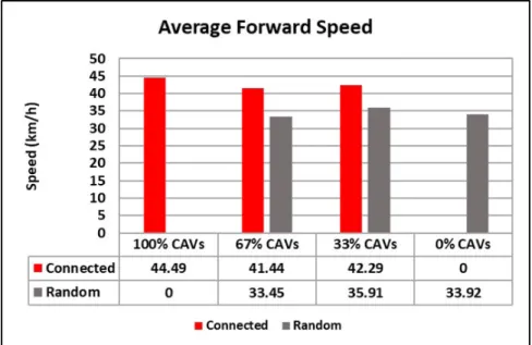
Figure 3: Average forward speed of connected and random vehicles
3.6
Observations
Clearly, the connected vehicles consistently maintained a higher speed (Figure 3) along the track than the randomly-changing vehicles in all situations. From observing the simulation runs it was obvious that the random vehicles made suboptimal lane-change decisions, often changing into slower lanes whereas the connected vehicles consistently bypassed those potential slowdowns. Although the maximum traffic density was limited by my simulation hardware, I believe that the speed improvement of the connected vehicles should carry over to some-what denser roads as well. If the density became much higher, I would change the default value ofQvto the pessimistic default to discourage speculative lane
changes when there are no-leaders nearby.
Driving comfort cost (Figure 4) was not as clear-cut. The random vehicles had a slightly lower average comfort cost, but the difference was significantly smaller than the difference in speed. In addition, this average cost is much more sensitive to a few specific parameter values than the difference in average speed: the random vehicles could have been made more likely to change lanes by increasingpland pr, or the connected vehicles could have been made more
“stingy” by adjusting the weights and thresholds of the reward functionsrCL
and rCR. Regardless, it seems that the slightly more lane changes that the
connected vehicles took were well worth it, judging by their much higher average speeds.
If we compare against the results in [2], our results are surprisingly favor-able. At low traffic densities like those in our simulation, Han et al. observed an increase of around 0-20% in traffic flow (a constant multiple of average veloc-ity) versus the baseline non-communicating vehicles. Our results were actually stronger, although this can likely be explained by two factors. First, our baseline agent changed lanes completely randomly, whereas theirs may have made more intelligent decisions. Second, our traffic density was lower than even their lowest experimental setting, which may have given the connected vehicles more time and space to maneuver through lanes. Unfortunately, for the reasons described above, we did not see a decrease in average comfort cost comparable to theirs (in fact, we saw the opposite). However, since the comfort cost function grows only with acceleration and number of lane changes, the comfort cost should not be confused for the “goodness” of the lane changing. The higher average com-fort cost of our connected vehicles was likely just due to the specific parameter values chosen.
3.7
Other Remarks
Several observations during earlier trial runs helped me identify limitations and make improvements to the algorithm. The idea to restrict Qv to only
con-sider vehicles in front (rather than all neighbors within distance ) came after watching vehicles in a prior version make poor decisions after other vehicles behind them changed speed. Similar to a human driver, it became clear that an autonomous driver should place much more importance on the environment
in front of them. Additionally, it took several iterations to find a satisfactory safety checking procedure usingHc,Hl, andHr. Unlike this work, [2]’s
simula-tion used MPC controllers and more shared informasimula-tion, which made the safety task easier in that work.
Even though the average vehicle speeds were fairly low, the PID controllers did not perform as well as I had hoped–there were infrequent vehicle collisions in some simulation runs that I believe most likely resulted from the controller not tracking the reference path well. This source of error could be improved by substituting in a more advanced controller like MPC, but that would introduce additional computational cost that would be difficult to test on my hardware. However, it would be necessary before testing on real vehicles in the future.
On the whole, the experiment clearly demonstrated the benefits of Algorithm 1 relative to the baseline and confirmed the potential for information-sharing to improve lane changing decisions. I believe that future work with more advanced methods will continue to produce increasingly stronger results.
4
Reflection
Algorithm 1 achieved my goal of showing measurable performance improvement over the baseline. It was able to do this with very little information sharing and had some notable advantages over the original algorithm in [2]. In addition, hardware limitations held the test environment back from achieving even better results (e.g. by replacing PID with MPC).
With that said, I acknowledge that this experiment was held in a very con-trolled environment (an open freeway with clean, dry roads and no obstacles). Real-world driving is much messier and vehicles must be able to handle a slew of different conditions. By making greater use of shared information or sensor inputs, there is plenty of room to continue improving lane-changing decisions. The results in Section 3 demonstrate that even without these “luxuries”, we can still find some resonable performance from limited information sharing.
More importantly, this project creates a solid platform for future research on CAV behavior planning. The software repository I produced will be reused for future algorithm testing by our lab. Further research and prototyping of different approaches will be accelerated by using my codebase. Hopefully, this will be even more valuable than the results in this report.
Working with an open-source project was not something I was accustomed to, so I gained lots of experience with new tools and workflows during this project. At times, debugging software without documentation forced me to become very resourceful. I also spent a significant amount of time reading essential background knowledge about control theory, vehicle dynamics, and mathematical optimization. These skills will help me dig deeper as I take on more complex projects in the future. This project served as a fantastic senior capstone to conclude my time in UConn Honors.
References
[1] Saeed Asadi Bagloee, Madjid Tavana, Mohsen Asadi, and Tracey Oliver. Au-tonomous vehicles: challenges, opportunities, and future implications for trans-portation policies. Journal of Modern Transportation, 24(4):284–303, 2016. [2] S. Han, J. Fu, and F. Miao. Exploiting beneficial information sharing among
autonomous vehicles. In 2019 IEEE 58th Conference on Decision and Control (CDC), pages 2226–2232, 2019.
[3] DSRC Committee et al. Dedicated short range communications (dsrc) message set dictionary. SAE Standard J, 2735:2015, 2009.
[4] P. Nilsson, O. Hussien, A. Balkan, Y. Chen, A. D. Ames, J. W. Grizzle, N. Ozay, H. Peng, and P. Tabuada. Correct-by-construction adaptive cruise control: Two approaches.IEEE Transactions on Control Systems Technology, 24(4):1294–1307, July 2016.
[5] J. Ploeg, D. P. Shukla, N. van de Wouw, and H. Nijmeijer. Controller synthesis for string stability of vehicle platoons. IEEE Transactions on Intelligent Trans-portation Systems, 15(2):854–865, April 2014.
[6] Brian Paden, Michal Cap, Sze Zheng Yong, Dmitry Yershov, and Emilio Frazzoli. A survey of motion planning and control techniques for self-driving urban vehicles.
IEEE Transactions on Intelligent Vehicles, 1(1):33–55, 2016.
[7] Yongsoon Yoon, Jongho Shin, H. Jin Kim, Yongwoon Park, and Shankar Sastry. Model-predictive active steering and obstacle avoidance for autonomous ground vehicles. Control Engineering Practice, 17(7):741–750, 2009.
[8] Y. Kanayama, Y. Kimura, F. Miyazaki, and T. Noguchi. A stable tracking control method for an autonomous mobile robot. InProceedings., IEEE International Conference on Robotics and Automation, pages 384–389 vol.1, 1990.
[9] Alexey Dosovitskiy, Germ´an Ros, Felipe Codevilla, Antonio L´opez, and Vladlen Koltun. CARLA: an open urban driving simulator.CoRR, abs/1711.03938, 2017. [10] M. Dupuis, E. Hekele, and A. Biehn. Opendrive format specification revision 1.5.