San Jose State University San Jose State University
SJSU ScholarWorks
SJSU ScholarWorks
Master's Projects Master's Theses and Graduate Research
Fall 12-16-2019
Assessing Wildfire Damage from High Resolution Satellite
Assessing Wildfire Damage from High Resolution Satellite
Imagery Using Classification Algorithms
Imagery Using Classification Algorithms
Ai-Linh AltenFollow this and additional works at: https://scholarworks.sjsu.edu/etd_projects
Assessing Wildfire Damage from High Resolution Satellite Imagery Using Classification Algorithms
A Project Report Presented to
The Faculty of the Department of Computer Science San Jos´e State University
In Partial Fulfillment
of the Requirements for the Degree Master of Science
by Ai-Linh Alten December 2019
© 2019 Ai-Linh Alten ALL RIGHTS RESERVED
The Designated Project Committee Approves the Project Titled
Assessing Wildfire Damage from High Resolution Satellite Imagery Using Classification Algorithms
by Ai-Linh Alten
APPROVED FOR THE DEPARTMENT OF COMPUTER SCIENCE
SAN JOS ´E STATE UNIVERSITY
December 2019
Dr. Ching-seh Wu, Ph.D. Department of Computer Science Dr. Teng Moh, Ph.D. Department of Computer Science Dr. Eric Waller, Ph.D. U.S. Geological Survey
ABSTRACT
Assessing Wildfire Damage from High Resolution Satellite Imagery Using Classification Algorithms
by Ai-Linh Alten
Wildfire damage assessments are important information for first responders, govern-ment agencies, and insurance companies to estimate the cost of damages and to help provide relief to those affected by a wildfire. With the help of Earth Observation satellite technology, determining the burn area extent of a fire can be done with traditional remote sensing methods like Normalized Burn Ratio. Using Very High Resolution satellites can help give even more accurate damage assessments but will come with some tradeoffs; these satellites can provide higher spatial and temporal resolution at the expense of better spectral resolution. As a wildfire burn area cannot be determined by traditional remote sensing methods with higher spatial resolution satellites, the use of machine learning can help predict the extent of the wildfire. This research project proposes an object-based classification method to train and compare several machine learning algorithms to detect the remaining burn scars after the event of a wildfire. Then, a building damage assessment approach is provided. The results of this research project shows that random forests can predict the burn scars with an accuracy of 86% using high resolution image data.
Keywords—Very High Resolution, wildfire burn severity, damage assessment, machine learning, Geographic Information Systems, remote sensing.
ACKNOWLEDGMENTS
I would like to thank my advisor, Professor Mike Wu, for helping me make this project a success, for being the best cheerleader in both my schooling and job applications, and for appreciating my love for the geospatial data sciences.
I would also like to thank my committee members, Professor Teng Moh and Dr. Eric Waller, for being the most wonderful teachers in my AI and remote sensing classes. With their guidance and amazing class curriculum, a lot of what I have learned has been put forth in this project.
I would like to thank Professor Shawn Newsam and my friends at the UC Merced Computer Vision Lab for their support during my undergraduate studies and for introducing me to GIS and digital image processing.
I also give credit to my mentor from DigitalGlobe, Mike Gleason, for helping me realize my careerpath in geospatial data science and for giving me the idea to pursue wildfires as my project topic.
Last, but not least, I would like to thank my parents for being so supportive throughout my undergraduate and graduate studies. I thank my father for helping me learn how to use AWS and Spark for this project. I also thank my loving mother for helping me get through every night by feeding me yogurt with frozen blueberries—full of the essential antioxidants to fuel the brain.
TABLE OF CONTENTS
1 Introduction. . . 1
2 Background and Related Work . . . 4
2.1 Burn Severity . . . 4
2.1.1 Feature Extraction . . . 5
2.1.1.1 Remote sensing features . . . 5
2.1.1.2 Image segmentation . . . 6
2.1.1.3 Image gradient orientation . . . 7
2.1.2 Classification Algorithms . . . 8 2.1.2.1 Preprocessing . . . 9 2.1.2.2 Feature selection . . . 9 2.1.2.3 SVM . . . 11 2.1.2.4 Random forests . . . 11 2.1.2.5 Other algorithms . . . 12
2.2 Damage Assessment Methods . . . 13
2.2.1 Map Visualization . . . 14
2.2.1.1 Semantic segmentation . . . 14
2.2.1.2 Color-coded building polygons. . . 15
2.2.1.3 Thematic maps . . . 16
3 Technical Approach . . . 18
3.1 Three Experiments: Binary, Multi-class Classification, and Spark . . . . 18
3.2 Python Modules. . . 20
3.3 Development Platform . . . 21
3.3.1 Local Desktop . . . 21
3.3.2 AWS EC2 for Scikit-Learn . . . 22
3.3.3 AWS EC2 for Spark . . . 22
4 Data Collection and Processing . . . 23
4.1 Areas of Interest . . . 23 4.2 Satellite Sources . . . 24 4.2.1 WorldView-3 . . . 24 4.2.2 Sentinel-2 . . . 25 4.3 Data Processing . . . 26 4.3.1 Preprocessing. . . 26 4.3.1.1 Atmospheric compensation . . . 26 4.3.1.2 Clip images . . . 28
4.3.1.3 Rescale and linear contrast stretch . . . 28
4.3.2 Data Transformation . . . 31
4.3.2.2 Vectorize image segments . . . 32
4.3.2.3 Feature extraction . . . 32
4.3.3 Final Dataset . . . 34
5 Experimental Design . . . 37
5.1 Experiment #1: Binary Classification . . . 37
5.1.1 Cross-Validation . . . 37
5.1.2 Evaluation . . . 38
5.1.3 Hyperparameter tuning . . . 39
5.2 Experiment #2: Multi-class Classification. . . 40
5.2.1 Cross-Validation . . . 41
5.2.2 Evaluation . . . 42
5.2.3 Hyperparameter tuning . . . 43
5.3 Experiment #3: Multi-class Classification with Spark . . . 44
5.3.1 Evaluation . . . 45
5.4 Map Visualizations . . . 46
5.4.1 Damage Assessment Map of Paradise, CA . . . 48
5.4.2 Burn Severity Map of Santa Rosa, CA . . . 49
6 Discussion of Results . . . 52
6.1 Comparing Classification Algorithms . . . 52
6.1.1 Random Forests and Decision Trees . . . 52
6.1.2 Multi-Layer Perceptron . . . 53
6.1.3 K-Nearest Neighbors . . . 53
6.1.4 Naive Bayes . . . 53
6.1.5 Models with One-vs-Rest and One-vs-One . . . 54
6.1.5.1 SVM . . . 54
6.1.5.2 Logistic regression and stochastic gradient descent . . . 54
6.2 Results and Comparisons with Existing Methods . . . 54
6.3 Thoughts on Spark . . . 55
7 Conclusion and Future Work . . . 57
List of References . . . 59
Appendix A: Confusion Matrices . . . 64
A.1 Experiment #1: Binary Classification Confusion Matrices . . . 64
A.2 Experiment #2: Multi-class Classification Confusion Matrices . . . 67
Appendix B: Exploratory Data Analysis. . . 72
B.1 Separability of the Classes . . . 73
LIST OF TABLES
Table 1. Image Gradient: Prewitt Operator . . . 8
Table 2. Selected Features . . . 10
Table 3. Classification Algorithms and Results . . . 13
Table 4. Satellite Sources Specifications . . . 27
Table 5. Cross-Validation Results for Binary Classification . . . 38
Table 6. Binary Classification Evaluation Scores . . . 39
Table 7. Cross-Validation Results for Multi-class Classification . . . 42
Table 8. Multi-class Classification Evaluation Scores . . . 43
Table 9. Spark Cross-Validation and Test Results . . . 46
LIST OF FIGURES
Fig. 1. Organization diagram of the literature review. . . 4
Fig. 2. Different levels of image segmentation. . . 7
Fig. 3. Map visualization examples for damage assessments. . . 15
Fig. 4. Methods for the wildfire damage assessment. . . 19
Fig. 5. The four steps taken in each experiment. Only the Spark experiment will go through first three steps. . . 20
Fig. 6. WorldView-3 image histograms of Paradise. . . 29
Fig. 7. Sentinel-2 image histograms of Paradise. . . 30
Fig. 8. SLIC Image segmentation example on Paradise pre-fire image. . . 31
Fig. 9. Preview of the intial GeoDataFrame. . . 32
Fig. 10. Example of regionprops and zonal statistics. . . 33
Fig. 11. Preview of the complete GeoDataFrame. . . 34
Fig. 12. Examples of land class. Photos from WorldView-3 of the Camp Fire. 35 Fig. 13. Table and bar chart that shows the number of segments per land and burn class. . . 36
Fig. 14. Random and grid search results for binary classification. . . 41
Fig. 15. The distribution of train and test sets used in multi-class classification. 41 Fig. 16. Random and grid search results for multi-class classification. . . 44
Fig. 17. An example of a single row in the LIBSVM file format. . . 45
Fig. 18. Pixel-wise classification flowchart. . . 47
Fig. 19. Building damage assessment map of Camp Fire. . . 48
Fig. 20. A closer look at a neighborhood within Paradise. . . 49
Fig. 21. A comparison of two image masks of Paradise. (Left) binary image mask with burn predictions. (Right) multi-class map. . . 50
Fig. 22. Post-fire image of Sonoma with binary mask. . . 51
Fig. 23. Confusion matrices with burn class . . . 64
Fig. 24. Confusion matrices with burn class (cont.) . . . 65
Fig. 25. Confusion matrices with burn class (cont. 2) . . . 66
Fig. 26. Confusion matrices with multi-class . . . 67
Fig. 27. Confusion matrices with multi-class (cont.) . . . 68
Fig. 28. Confusion matrices with multi-class (cont. 2) . . . 69
Fig. 29. Confusion matrices with burn class (cont. 3) . . . 70
Fig. 30. Confusion matrices with burn class (cont. 4) . . . 71
Fig. 31. Average Digital Number value of the binary burn class and multi land use class in each VNIR band obtained from the post-fire Paradise image. . . 72
Fig. 32. Class distributions of NDVI. . . 74
Fig. 33. Pair plot feature space of post-fire SIs. . . 76
1 INTRODUCTION
The news of wildfires spreading in the Western United States has caught the attention of many people nationally and internationally. According to the Congressional Research Service (CRS), wildfires have increased every year dramatically since the 1990s. The annual average of land burned in the 1990s was 3.3 million acres, in the 2000s it was 6.9 million acres, and in recent years it gets as high as 10 million acres [1]. The Western U.S. is especially susceptible to combustion due to hot temperatures and dry vegetation [2]. In 2017 and 2018, California experienced some of the most destructive fires in which many homes and lives were lost. Cal Fire [3] reported that the October 2017 Tubbs Fire and November 2018 Camp Fire destroyed 5,636 and 18,804 homes respectively. However, getting rapid information about the estimated wildfire damages in urban areas is not always easy. Firefighter Nation [4] discusses several wildfire detection surveillance technologies: ground-based visual systems, ground-based non-visual sensors, manned and unmanned aircrafts, and satellites. Each surveillance technology comes with unique challenges like the cost of direct human operability, wide-area coverage, massive data storage, and good temporal frequency.
Of these surveillance technologies, Very High Resolution (VHR) Earth Observation (EO) satellites are a good data source that can provide highly accurate damage assessments at spatial scales between 0.3 to 2 meters. EO satellites solve the problem of direct human operability and temporal frequency in order to provide faster decision making [5]. Commercial satellite companies are now moving their satellite images into the cloud in response to the “Big Data” issue of data storage and management [5]. VHR satellites capture multispectral images between the visible light range and near-infrared of the electromagnetic spectrum (VNIR). Although VHR satellites capture images at incredibly high resolutions, they cannot provide burn severity assessments via traditional remote sensing methods without the availability of short-wave infrared (SWIR). For the past
decade, a trend of machine learning classification algorithms has been able to provide wildfire burn severity assessments. These algorithms look for returns from the carbon stocks on land in the visible red and NIR range [6].
To make up for the lack of the SWIR in VHR imagery, this research project proposes an object-based classification method using supervised machine learning algorithms to determine the burn severity with only the VNIR bands. The high resolution satellite images are first broken up into segments via an image segmentation algorithm called Super Linear Iterative Clustering (SLIC) that groups pixels by color similarity and spatial proximity [7]. These segments are then used to extract the band values and the spectral indices from the satellite imagery as the features. Following the creation of the new dataset, three main experiments using several classification algorithms provided by Scikit-Learn and Apache Spark will be evaluated and compared. The first experiment will judge if binary classification will be sufficient to identify if the land has been burned. The second will determine if multi-class land use classification will be possible with just the VHR imagery. And lastly, if prior classification methods will be able to justify the need to use a distributed system like Spark for training and making predictions on large amounts of satellite data. Once the best classification algorithm is selected from the binary classification and multi-class classification experiments, the model will be used to prepare map visuals of the burn scar and land usage. This research project will also propose a workflow for creating the building damage assessment maps.
This report will be organized as follows. Chapter 2 will go over the current state-of-the-art burn severity methods using classification algorithms. This section will also review several literature that propose different map visualization methods for building damage assessments. Chapter 3 will then go over the technical approach for the project as well as the development environments used. The motivation behind the selection of the satellite image data collection will be discussed in Chapter 4. Image preprocessing
and data transformation methods will be presented in Chapter 4.3. Chapters 5.1–5.3 will go over the results from the three experiments using Scikit-Learn and Spark. The map visualization methods will be proposed in Chapter 5.4. Lastly, Chapter 6 will discuss the results from the three experiments and conclude in Chapter 7.
2 BACKGROUND AND RELATED WORK
This background study and review will survey the various classification algorithms that help create burn severity maps. It will also discuss methods to provide map visuals using Geographical Information Systems (GIS). Two questions will be answered in this review: What features and classification algorithms using a single satellite image data source will be suitable for providing wildfire burn severity? How should the damage assessment be conducted for a suitable visualization that accurately represents the information? The research papers reviewed will be split into two main parts: burn severity and damage assessments. A breakdown of the review is shown in Fig. 1.
Fig. 1: Organization diagram of the literature review.
2.1 Burn Severity
Burn severity describes the results after a fire has burned by reporting the loss of vegetation, amount of water content in the soil, and discoloration of the soil. Levels of burn severity—high, medium, and low—make up the burn area. Burn severity can also be represented by many subclasses between the soil and tree canopies usually with five strata per the Composite Burn Index (CBI) [6]. CBI is well understood by experts in
ecology. For the focus of this study, burn severity will be used to help provide the damage assessment.
Machine learning algorithms are statistical algorithms that try to approximate what the overall population is given a subsample. Machine learning makes predictions based on what it has learned about the population. As an example, the population is all wildfires in the U.S. that have occurred, and a subsample could be the Camp Fire that occurred in November of 2018 in Paradise, California. Classification algorithms are supervised learning models that predict discrete classes of objects. They learn off predictor variables that describe the population. In remote sensing, several classification algorithms are suggested by Holloway and Mengersen [8]: logistic or multinomial regression, support vector machines, classification and regression trees (CART), random forests (RF), K nearest neighbor (k-NN), pixel classification like spectral mixture analysis (SMA), and neural networks. In the following sections, feature extraction methods for useful predictor variables will be explored as well as a few studies that create burn area maps using classification algorithms.
2.1.1 Feature Extraction
In this section, papers discussing feature extraction for burn severity and damage assessments are covered. There are three main features that will be discussed for feature extraction. First, remote sensing features can potentially provide the spectral information necessary to determine the extent of the wildfire burn. The other two features involve image processing techniques. The feasibility of using image segmentation for object-based classification and image gradient orientation for determining the spatial characteristics of the burned vegetation will be explored.
2.1.1.1 Remote sensing features: There are many feature extraction methods for image classification using the spectral information of satellite data. Meng and Zhao [6] summarized many of these methods from other sources. They have found that many burn
severity methods use some of the following: spectral signatures, spectral indices (SIs), and endmembers by spectral unmixing. Meng and Zhao [6] suggests that changes in spectral signatures are seen by the reduced water content of the vegetation in the visible NIR and mid-infrared (MIR) range. For SIs, many vegetation spectral indices were used like Normalized Difference Vegetation Index (NDVI), Enhanced Vegetation Index (EVI), Soil Adjusted Vegetation Index (SAVI), Modified SAVI (MSAVI), and Integrated Forest Index (IFI).
SI=band1−band2
band1+band2 (1)
Newer bi-temporal SIs like Normalized Burn Ratio (NBR), differenced NBR (dNBR), and relative dNBR (RdNBR) were popularized for identifying the change in pre- versus post-fire imagery [6].
dSI=SIpre−SIpost (2)
Endmembers were used for a classification technique called Spectral Mixture Analysis (SMA) which describes the spectrum’s distribution and defines endmembers by class like soil and vegetation [6].
Equations 1 and 2 shows examples of the normalized difference ratio equations. SI takes the difference of two bands (band1 and band2) selected from the satellite image and then normalizes to a range of -1 to 1.dSI is the change between the pre-event and post-event image. For example,NDV I=NIRNIR+Red−Red anddNDV I=NDV Ipre−NDV Ipost.
2.1.1.2 Image segmentation: Mitri and Gitas [9] provided a feature extraction technique using image segmentation in order to classify burn severity. In their methodology, they segmented an IKONOS satellite image and classified the segmented objects via fuzzy logic. The image segmentation is done using a bottom-up region-merging algorithm in order to provide three levels of segmentations in the image [9, Fig. 2]. This segmentation and merging technique in remote sensing is known as Object-based Image Analysis
(OBIA). What image segmentation algorithm [9] used is not mentioned, but it can be assumed it is an algorithm that can only use visible color bands since IKONOS is only a 4-band sensor (red, green, blue, NIR). A more recent study by Wang et al. [10] describes a deep hierarchical representation and segmentation approach for high resolution satellite images. This paper uses a fast scanning image segmentation via deep learning to split and merge segmented regions [10]. This way, segmentation is robust for any spatial scale and can represent the different types of vegetation between canopy to surface. Region Adjacency Graph (RAG) is used to determine how the merging is done hierarchically by relating the border elements. This region merging of segments is done in a bottom-up fashion as well [10]. With image segmentation, this can be used to provide an object-based classification method rather than pixel-based. Segments can represent a variety of things like trees, buildings, water, etc.
Fig. 2: Different levels of image segmentation. Source: [9].
2.1.1.3 Image gradient orientation: Although the primary focus for extracting features will be for burn severity, it is also important to know the spatial characteristics that come with vegetation as well as damaged buildings within areas of dense vegetation. Ye et al. [11] proposes a method to detect damaged buildings from earthquakes using a feature
called Local Gradient Orientation Entropy (LGOE). They found that the probability of multiple gradient orientations is greater for a damaged building than for an intact building. This way, shadows of the building don’t need to be used as a feature since it is influenced by solar elevation, weather condition, and distance between the buildings [11]. LGOE is a Prewitt gradient operator Table 1 used locally within each building. Angles chosen are a step of 15 degrees between 0 and 180 degrees [11]. Oriented gradients could be a good predictor variable for both vegetation and buildings affected by a forest fire. Other known image gradient operators that can be used are Sobel, Robert, and Laplace. Histogram of Oriented Gradients (HOG) and Gabor filters can also be used as textures for a feature descriptor.
Table 1: Image Gradient: Prewitt Operator
Horizontal orientation Vertical orientation Mask −10 −10 −10 1 1 1 1 1 1 0 0 0 −1−1−1 Image Result 2.1.2 Classification Algorithms
For the past ten years, a trend of machine learning algorithms has been used for identifying burn areas in satellite images. Some algorithms used are principal component analysis (PCA), support vector machines (SVM), neural networks (NN), convolutional neural network (CNN), deep belief network (DBN), autoencoder, spectral angle mapper (SAM), random forests, and decision trees [6], [12]. In this review, six journal articles [13]– [18] providing wildfire burn severity are classified by the following algorithms: SVM,
artificial neural networks (ANN), SAM, Gaussian process regression (GPR), support vector regression (SVR), and RF. The following sections will also cover the steps in the data mining process from these articles.
2.1.2.1 Preprocessing: Off the sensor, images from satellites are affected by atmospheric conditions, sun angle, and cloud cover which need to be retouched in order to make the image real color. Geometric corrections are also required if the image is taken off-nadir. Off-nadir is the angle between how the satellite is positioned and surface of the Earth during the scanning process. Although many providers of satellite images like Google Earth Engine makes the correction for these images automatically, many others provide only raw images that need preprocessing. For atmospheric correction (aka. radiometric conversion), several studies [15], [16], [18] used dark object subtraction to reduce the absorption and scattering of light energy as it passes through the Earth’s atmosphere. Fixing illumination is done topographically, minimizing view-angle brightness, cloud masks, and water masks [15], [18]. Merging multiple images is done by data fusion and image mosaicking [15], [16]. Orthorectification also helps remove the effects of off-nadir by making the image more planimetrically correct [16]. In [17], data reduction of pixels is resolved by removing any unburned vegetation pixels that are more than 3,000 m from burned pixels. This helps with the spatial autocorrelation problem when neighboring pixels are unrelated.
2.1.2.2 Feature selection: Many features as described in Section 2.1.1 are used for the classification of burn severity. These predictor variables Table 2 are either represented as a pixel or an object for pixel-based [13], [14], [16], [17] and object-based classification [15], [18]. Although most methods used post-fire images for representing the reflectance and spectral indices, some research calls for the use of both pre-fire and post-fire images in order to use dSIs between two image dates [16], [17]. The last column in Table 2 shows which satellite sensor is used for the features. This determines what radiance values and
SIs will be used. It is preferable to use multispectral VHR satellites for the goal of this research, however [15], [17] show the use of hyperspectral satellites for burn severity classification. Meng et al. [16] use Multiple Endmember Spectral Analysis (MESMA) procedure to determine an endmember spectra library for burned and non-burned oak, pine, wetland, shrub, and grass. Hultquist et al. [15] describes the use of internal image texture (TXIT) and neighborhood texture (GEOTEX) within each image segment. Ramo et al. [17] uses Euclidean distance between pixels and wildfire burn hotspots for spatial correlation.
Table 2: Selected Features
Name Reflectance
value SIs dSIs Endmember
Image gradients EO sensor(s) G.P. Petropoulous et al. [13] X Landsat-5 TM G.P. Petropoulous et al. [14] X Landsat-5 TM C. Hultquist et al. [15] X X X MASTER R. Meng et al. [16] X X WorldView-2, LiDAR, Thermal LiHT
R. Ramo et al. [17] X X X MODIS
L. Collins et al. [18] X X
Landsat-5 TM, 7 ETM+, 8 OLI/TIR
Some research used dimension reduction techniques to reduce the number of predictor variables before training the classification algorithms. Hultquist et al. [15] suggests using minimum redundancy feature selection (mRMR) to rank the predictor variables in terms of ability to predict the correct class. They found that TXIT, GEOTEX, NBR, NDVI, and a few radiance values best correlated to CBI [15]. Meng et al. [16] chose the top eight SIs using separability analysis. Ramo et al. [17] merged the results of features selected
by the Boruta RF algorithm, logistic regression, and an Entropy-based filter to keep for training classification algorithms. Of the eight features selected by their method, the top features were NDWI, NBR, and hotspot distance [17]. Collins et al. [18] used Gini Impurity statistic and found that dNDWI and dNDVI had the greatest influence on the RF classifier. According to the feature selection methods, SIs, dSIs, and image textures will be valuable predictors for model construction.
2.1.2.3 SVM: Several kernel-based algorithms were suggested to perform multiclassification on burn severity classes. SVM for classification, SVR for regression, and GPR is used among many works providing burn area mapping as shown in Table 3 [13], [15], [18]. SVM is a supervised algorithm that linearly separates classes with a hyperplane by minimizing the margin between them. Petropoulos et al. [13] suggests using a pair-wise binary classification strategy to classify the following types of land cover: burn area, agricultural, scrubland, forested, and urban. With a train and test split of 180 and 60 pixels per class, they trained and tested the SVMs on several kernels: polynomial, radial basis function, and sigmoid [13]. In their test, they had 95.87% overall accuracy and 0.948 kappa coefficient. Their burn area class had 100% accuracy using SVM [13]. SVR handles non-linear problems by using a different kind of slack variable to perform regression [15]. GPR is like SVR but has a Bayesian context and infers functional relationships from the training data [15]. Hultquist et al. [15] compares both SVR and GPR on MASTER image plots labelled by CBI values. SVR and GPR had RMSE values of around 0.30 to 0.35. The use of SVMs shows promise in identifying burn area as well as other kinds of land cover classes. However, according to the results in [15], random forests were able to outperform both SVR and GPR.
2.1.2.4 Random forests: Random forests (RFs) is the most commonly used burn severity classification algorithm [15]–[18]. RFs are an ensemble of decision trees that can assign a class by voting for categorical data or averaging for continuous data [18].
Collins et al. [18] analyzed 16 fires in Victoria, Australia from pre- and post-fire Landsat imagery using the RF classifier in R and visualized with Google Earth Engine (GEE). From 16 fires, a sample 10,855 pixels were generated, and nine SIs were used as features — each pixel labelled as unburnt, crown unburnt, partial crown scorch, crown scorch, and crown consumption. Collins et al. [18] tested the model stability using 16-fold cross validation where one fire is left out in each iteration. With 95% confidence, they were able to determine the overall training accuracy as 91% and overall testing accuracy as 85% [18]. Their results show that SIs and dSIs are very promising variables to use in training data for the RF model. Hultquist et al. [15] and Ramo et al. [17] used similar techniques and were able to show that RF could outperform many other algorithms like multiple regression, SVM, SVR, and ANN. Meng et al. [16] preferred a hybrid approach including multiple datasets with the multispectral satellite data — including LiDAR and Thermal infrared to generate more SIs and endmembers that represent burned vegetation. Although their classification accuracy of 84% looks promising, the use of external data sources beyond a single satellite platform can be complicated and will require many preprocessing and co-registration steps to align the different data sources. Most of the work is done manually rather than automatically [18].
2.1.2.5 Other algorithms: Many other algorithms were also explored in burn severity classification. ANN, SAM, multiple regression, and C5.0 to name a few [14], [15], [17]. ANNs are a composed of simple processing units and are designed like neurons interconnected in a brain. Petropoulos et al. [14] uses a multi-layered feed-forward ANN with a logistic activation function to delineate burn area and classify other land cover types from Landsat imagery in ENVI software. This is compared to SAM which is a spectral classifier that can determine similarity in image spectra by calculating the angles between them. Small angles indicate high similarity and large angles indicate low similarity [14]. ANN had an accuracy of 90.29% overall and outperformed SAM which had 83.82% [14].
Table 3: Classification Algorithms and Results Name ML algorithms Cross-validation Accuracy G.P. Petropoulous et al. [13] SVM N/A 95.76% overall G.P. Petropoulous et al. [14] ANN; SAM N/A 95.29% overall; 83.82% overall C. Hultquist et al. [15] Multiple regression; RF; SVR; GPR Grid search, empirical Bayes 0.54 RMSE; 0.28 RMSE; 0.38 RMSE; 0.39 RMSE
R. Meng et al. [16] RF N/A 84% overall
R. Ramo et al. [17] RF; SVM; ANN; C5.0 N/A 0.42 CE, 0.43 OE; 0.17 CE, 0.81 OE; 0.05 CE, 0.75 OE L. Collins et al. [18] RF 16-fold 87% overall
According to Hultquist et al. [15], multiple regression is typically a commonly used algorithm for non-linear prediction on predictor variable like CBI. Compared to RF, SVR, and GPR, it had the worst performance [15]. An almost unheard-of algorithm in burn severity classification, C5.0, is used by Ramo et al. [17] as it can estimate the probability of burned area. C5.0 uses a gain ratio criterion to select important attributes during tree construction. It outperformed SVM and ANN and was able to have good performance similar to RF [17].
2.2 Damage Assessment Methods
Damage assessments report the losses after an accident or natural disaster. They estimate what can be restored, and how much time and cost it will take for recovery. This helps the government, first-responders, insurance companies, and others to help evacuate, shelter, and replace what is lost [19]. For the focus of this study, building and structure
damage assessments will be explored to report on the estimated number of damaged and destroyed buildings in residential areas.
2.2.1 Map Visualization
In the following sections, building damage assessment visualization methods via image-based and vector-based will be reviewed. Most current building damage assessment techniques are for earthquakes rather than wildfires. However, the methods described by [11], [20]–[24] will be applicable for wildfires as well.
2.2.1.1 Semantic segmentation: Georeferenced raster data can provide for a way to visualize results from semantic segmentation. A damage assessment study by Trekin et al. [20] uses VHR imagery from DigitalGlobe’s OpenData program that provides pre- and post-fire images in December 2017 of the Thomas Fire that occurred in Ventura, Santa Barbara, California. Trekin et al. [20] prepared training data from Open Street Map’s (OSM) building layer and Google Map’s imagery that is 3-band with just a visible range of red, green, and blue channels. From the OSM vector, they create a 1-band pixel mask which is a picture of white pixels (building) and black pixels (no buildings). A semantic segmentation approach for change detection with CNN is trained on Google pre- and post-fire aerial images and OSM building pixel mask to make predictions on whether the building pixels have changed after the wildfire [20]. For visualization they used a semantic segmentation image map that shows that the black pixels as non-damaged buildings, gray pixels as damaged buildings, and white as everything else [20]. Using raster can be a good way to represent the map visual of whether buildings are destroyed or not; but with poor classification performance, some pixels may be randomly guessed which causes buildings to be disproportionate and have no clear separability between each other. This can be seen in the result after testing the pre-trained CNN on DigitalGlobe’s Open Data images when some buildings are either misclassified, merged with another building next to it, or show irregular shape [20, Fig. 3(a)]. Building vectors may be better suited for showing
(a) semantic segmentation (b) color-coded building polygons
(c) dasymetric map
Fig. 3: Map visualization examples for damage assessments. Source: [11], [20], [21].
the results of what buildings have been harmed or destroyed without ever changing the shape of the original building polygon.
2.2.1.2 Color-coded building polygons: Using color-coding on building polygons is the most popular of the visualization methods for building damage assessment [11], [22]–
[24]. It is the most intuitive to implement and easy to interpret. This kind of visualization is a good example of using both remote sensing data and vector data of building polygon data. Ye et al. [11] uses a Quickbird image (4-band with 0.61m resolution) after an earthquake in Yushu, China in 2010 and a vector of 101 buildings to provide the visual. A quick classification is done with LGOE to classify and color the buildings as damaged (red) and undamaged (blue). Buildings incorrectly classified are labelled as commission error (yellow) and omission error (purple) [11, Fig. 3(b)].
Their method had 86% overall accuracy when correctly classifying the damage status. Similarly, Sofina and Ehlers [22], [23] uses a Quickbird image over the same area but uses a Canny edge detector and grey co-ocurrence matrix to select buildings that have high frequency. Both k-means and k-NN is then used to perform a binary classification to label building vectors as intact or destroyed, giving them 78% and 84% overall accuracy. Guida et al. [24] demonstrates the use of Synthetic Aperature Radar (SAR) with building vector data. They perform a Coherent Change Detection algorithm to get point locations of changes within the images. The points are then intersected with the building polygons in order to classify as destroyed, highly damaged, moderately damaged, or negligible to slight damage [24]. Use of color-coding is very simple and can be used with a satellite image of the event as a base overlay. Building polygons will work well with small scale maps, however, may not be able to be visualized on larger scale maps. It may be necessary to provide an aggregated visual of the buildings at larger map scales like pie chart maps or thematic maps.
2.2.1.3 Thematic maps: The use of thematic maps can represent the number of damaged buildings within a geographical area. Miura et al. [21, Fig. 3(c)] provides a dasymetric map visual to represent the number of buildings that were destroyed during an earthquake in Metro Manila, Philippines in the year 2001. From IKONOS imagery, they came up with a time-series based land cover classification using edge detection
and a hybrid simulation method to get the capacity spectrum. It is unclear how the damage ratio is determined from their methodology, but it is multiplied to the number of buildings in each pixel (about three buildings per pixel) in order to get a heatmap-like result [21, Fig. 3(c)]. They were able to determine that about 180,000 buildings were destroyed. This method avoids the need of requiring a complete building vector data in order to produce a map. Miura et al. [21] points out that GIS data of buildings are not always up to date and available in many regions, as Manila had only 280,000 buildings in their 1987 GIS data whereas in 1989 it is estimated to have 910,000 buildings. So, it is important to continue to update the geodatabase of buildings in order to use it for a damage assessment.
Semantic segmentation, building polygons, and thematic maps are all good visualiza-tion techniques that can be useful for wildfire damage assessments. Rasters with semantic segmentation can provide a map visual but may not be easy to provide as a layer for WebGIS as they will typically need to be converted to web map tiles. Building vector layers can be for web map services and desktop GIS programs since it represents discrete data and is aesthetically pleasing. Vector layers also keeps the shape of the building polygons without ever altering it. Building vectors are not always available in every country or region. Hence, thematic maps can be a good replacement if there is no building vector data. However, it can provide an estimate of the number of buildings that have been destroyed in a wildfire.
3 TECHNICAL APPROACH
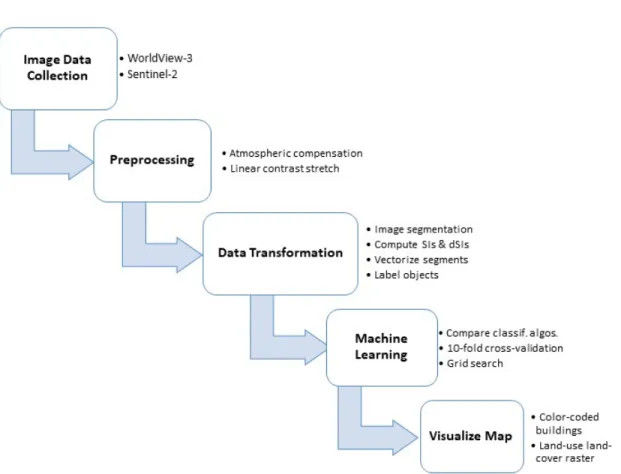
This chapter proposes the methods for assessing wildfire damage using high spatial resolution EO satellites. Fig. 4 gives an overview of the steps taken to make a wildfire damage assessment and will be discussed in the following chapters 4–5.4. First, Chapter 4 will discuss which satellite sensors and images were used for the experiments. Second, Chapter 4.3 will discuss the image preprossessing methods and methods to transform the data into objects to label for supervised learning. Next, several supervised machine learning algorithms will be compared in three separate burn severity classification experiments: binary classification, multi-class classification, and multi-class classification with Spark MLLib in chapters 5.1–5.3. Finally, providing a solution to visualize the map with GIS methods in Chapter 5.4.
3.1 Three Experiments: Binary, Multi-class Classification, and Spark
In this project, the three experiments for binary, class classification, and multi-class multi-classification with Spark are explored as possible ventures for determining burn severity with high resolution EO satellite imagery. The first experiment’s goal is to see if it is possible to determine separability between things that are burned by the fire and things that are not. The multi-class classification burn severity experiment is to understand the predictive ability of the models for various land usage types and its ability to detect the burned regions.
In the third experiment, the feasibility of using Spark MLLib for determining burn severity is also explored. Apache Spark is well known for its fast and efficient distributed data processing on Big Data. It is based off of the MapReduce distributed processing framework that can split data into chunks to distribute and to parallelize the computations across the cluster. Spark is made faster than MapReduce by caching data in memory and runs multi-threaded tasks in Java Virtual Machine (JVM) processes [25]. Spark is very suitable for handling Big Data at sizes larger than a petabyte. Spark MLLib
Fig. 4: Methods for the wildfire damage assessment.
makes use of the distributed data processing for training machine learning algorithms at scale [25]. Although the data used in this project is not large enough to be considered as Big Data, Spark should still be considered in any machine learning project involving copious amounts of EO data. This project will demonstrate a proof-of-concept using Spark for multi-class classification and determine if the algorithms and tools provided by MLLib will be sufficient for determining burn severity.
Fig. 5: The four steps taken in each experiment. Only the Spark experiment will go through first three steps.
In chapters 5.1–5.3, the steps taken to evaluate the binary classification and multi-class classification models will be the same for all three experiments as shown in Fig. 5. All models will be measured by their cross-validation performance and their test accuracy, precision, recall, and F1-scores. In the fourth step, the model that has the maximum precision score will be hyperparameter tuned. Only the third experiment with Spark will not be hyperparameter tuned.
3.2 Python Modules
Throughout the duration of this project, the Python programming language is used as it provides the most useful modules for geospatial data analysis. The following modules are used in this project:
• Scikit-Learn: a free software library providing an extensive set of tools for data mining and data analysis and is built on NumPy, SciPy, matplotlib, and joblib. This project uses many of its provided supervised learning algorithms such as random forests, SVM, k-NN, and multi-layer perceptron (MLP). Scikit-Learn also provides tools for k-fold cross-validation and hyper-parameter tuning via exhaustive grid search. Scikit-Learn does not provide many strategies for scaling for Big Data as most of the models will learn from data that fits on the main memory and only can do multi-core parallelism using the CPU [26].
• Scikit-image:a free collection of image processing algorithms. This project uses the SLIC segmentation algorithm, regionprops, and morphology libraries [27].
• Pyspark:the Python library for Spark. This utilizes Spark’s functionality of running independent processes on a cluster of nodes. Pyspark MLLib also provides a variety of classification algorithms and grid search for parameter tuning [28].
• Pandas and Geopandas:an open-source library with DataFrame objects for data manipulation with integrated indexing. The geospatial version, Geopandas, allows for storing Shapely geometry objects, such as Polygons, Points, and LineStrings [29]. Geopandas can read and write any vector files like GeoJSON and ESRI Shapefiles. • Geospatial modules
– Shapely: used to create Polygons.
– Pyproj and Fiona: used for projecting Shapely geometries into a new spatial reference.
– Rasterio: used for reading in satellite images and store as NumPy array objects. This supports any raster data extensions like GeoTIFF.
– GDAL: used for translating image data into Byte and perform a linear contrast stretch.
– Rasterstats: used for the zonal statistics function to overlay Shapely polygons onto a raster image and returns the specified statistic.
3.3 Development Platform 3.3.1 Local Desktop
During the first few stages of the project, this enviornment was used for data collection, data preprocessing and transformation, and for the first experiment on binary classification. This setup had the following specifications:
• Windows 10 x64-based • Intel Core i7 processor • 16 GB RAM
3.3.2 AWS EC2 for Scikit-Learn
For the machine learning stages of the project, AWS EC2 instances were used for cross-validating models, hyperparameter tuning, and for creating the predictions for map visuals. Joblib multi-core processing was utilized for maximum efficiency of the provided hardware in the EC2 instance. For cross-validation and hyperparameter tuning the following system is used:
• EC2 Type: c5.9xlarge
– 36 virtual CPUs
– 72 GB memory
– EBS-optimized storage
Then for making the predictions for the map visuals, the following EC2 instance was used: • EC2 Type: c5.24xlarge
– 96 virtual CPUs
– 192 GB memory
– EBS-optimized storage 3.3.3 AWS EC2 for Spark
Lastly, a Spark cluster with a master and slave node was created on AWS EC2 instances by an open-source tool called Flintrock. Data files used for Spark MLLib is stored in the Hadoop Distributed File System (HDFS). Each node had the following specifications:
• EC2 Type: m5ad2xlarge
– 8 virtual CPUs
– 32 GB memory
4 DATA COLLECTION AND PROCESSING
Many commercial EO satellite sensors provide VHR images at spatial resolutions 0.31m–2m [30]. When collecting the satellite image data, some criteria were kept in mind. According to Satellite Imaging Corporation [30], many high resolution EO satellites in orbit today sense the visible and near-infrared (VNIR) portion of the electromagnetic spectrum between wavelengths 450nm–950nm. Most commercial satellites offer one panchromatic band and four multispectral bands: blue, green, red, and near-infrared. Another motivation to use VHR commercial satellites is their ability to image the same area at a high temporal frequency between one to three days. In this section, the Areas of Interest (AOI) and satellite sources will be selected given the following criteria: images must be of recent fires with the highest number of destroyed structures, images must have four VNIR bands, and the satellite sensor have frequent revisit times.
4.1 Areas of Interest
In this project, two California wildfires were used as the AOIs. The Camp Fire in Butte County, the most destructive fire to date, burned about 149,000 acres of land and destroyed 18,804 buildings. This fire lasted between the dates November 8, 2018 to November 25, 2018 [3]. As this is quite a large area, most of the experiments were done over the city of Paradise. The selected satellite images over Paradise were used for the data creation and machine learning phases of the project.
The second AOI is the Tubbs fire of the October 2017 Northern California fires. This fire reached across Sonoma, Napa County, Lake, and Santa Rosa County, burned a total of 36,807 acres of land between October 8, 2017 to October 31, 2017. This fire destroyed a total of 5,643 structures [3]. The AOI selected is mostly centered around Coffey Park in the city of Santa Rosa and is used in an experiment in Chapter 5.4 to verify if the trained classification model has good predictability in an urban area.
4.2 Satellite Sources 4.2.1 WorldView-3
WorldView-3 is a commercial high resolution EO satellite that offers up to spatial resolutions of 31cm. DigitalGlobe (now Maxar Technologies), provides VHR satellite imagery through their Open Data Program for disaster response [31]. This archive includes pre-event and post-event imagery of the Camp Fire in 2018 and Tubbs Fire in 2017. Table 4 summarizes the specifications of the WorldView-3 satellite. Although WorldView-3 has an impressive number of spectral bands, the Open Data Program only provides data from their satellite sensors in the visible band range: red, green, and blue. All images provided by DigitalGlobe’s Open Data Program are also processed by orthorectification, atmospheric compensation, dynamic range adjustment, and pan-sharpening [32]. So by default, each image has already undergone an image histogram stretch and will be at 31cm spatial resolution. For this project the images for each AOI were selected:
• Paradise, CA
– Pre-fire image ∗ Date: 9/10/2018
∗ ID: 1040010042A1A800 ∗ Data type: Byte
∗ Coordinate System: EPSG 4326
– Post-fire image ∗ Date: 11/25/2018
∗ ID: 10400100455BCD00 ∗ Data type: Byte
∗ Coordinate System: EPSG 4326 • Santa Rosa, CA
∗ Date: 6/21/2017
∗ ID: 105001000A632800 ∗ Data type: Byte
∗ Coordinate System: EPSG 4326
– Post-fire image ∗ Date: 10/17/2017 ∗ ID: 1040010034141800 ∗ Data type: Byte
∗ Coordinate System: EPSG 4326 4.2.2 Sentinel-2
As the goal of this project is to be able to use high resolution EO satellite sensors in the VNIR spectrum, the need for a near-infrared band is critical in the experiments. As the DigitalGlobe Open Data Program does not offer a NIR band with their images, Sentinel-2 NIR images were collected from the Registery of Open Data on AWS [33]. Table 4 describes the specifications of Sentinel-2. Each Sentinel-2 NIR image has a spatial resolution of 10m and corrected by radiometric and geometric but has no atmospheric correction [34]. As Sentinel-2 has a revisit time of 5 days, the images chosen must fall within a week of when the WorldView-3 images were taken. The following images of each AOI were selected:
• Paradise, CA – Pre-fire image
∗ Date: 9/7/2018
∗ ID: S2B MSIL2A 20180907T184909 N0206 R113 T10TFK 20180907T224321
∗ Data type: 16-bit unsigned integer ∗ Coordinate System: EPSG 32610
– Post-fire image ∗ Date: 12/6/2018
∗ ID: S2B MSIL2A 20181206T185749 N0207 R113 T10TFK 20181206T203841
∗ Data type: 16-bit unsigned integer ∗ Coordinate System: EPSG 32610 • Santa Rosa, CA
– Pre-fire image ∗ Date: 6/19/17
∗ ID: S2A MSIL1C 20170619T184921 N0205 R113 T10SEH 20170619T185728
∗ Data type: 16-bit unsigned integer ∗ Coordinate System: EPSG 32610
– Post-fire image ∗ Date: 10/17/2017
∗ ID: S2A MSIL1C 20171017T185401 N0205 R113 T10SEH 20171017T185935
∗ Data type: 16-bit unsigned integer ∗ Coordinate System: EPSG 32610
4.3 Data Processing
This chapter proposes methods for preprocessing and data transformation. The purpose of these steps is to transform the satellite image data into Shapely Polygon objects that can be labelled for supervised learning.
4.3.1 Preprocessing
4.3.1.1 Atmospheric compensation: As satellites off-the-sensor are affected by atmospheric conditions, preprocessing the images is required to remove the haze-like
Table 4: Satellite Sources Specifications
Satellite Spectral res. Spatial res. Temporal
Freq. Other notes
WorldView-3 Panchromatic: 450–800nm 8 Multispectral Coastal: 397–454nm Blue: 445–517nm Green: 507–586nm Yellow: 580–629nm Red: 626–696nm Red Edge: 698–749nm NIR1: 765–899nm NIR2: 857–1039nm PAN: 0.31m MS: 1.85m daily Altitude: 617km,Orbit: sun-synchronous 10:30am descending node, Affiliation: Maxar Technologies Sentinel-2 13 Multispectral Coastal: 422–464nm Blue: 426–558nm Green: 524–596nm Red: 634–696nm Veg Red Edge: 689–719nm Veg Red Edge: 725–755nm Veg Red Edge: 760–800nm
NIR: 727–939nm Narrow NIR: 843.7–885.7nm Water vapour: 924–964nm SWIR-Cirrus: 1345–1405nm SWIR: 1519–1705nm SWIR: 2020-2380nm C: 60m B: 10m G: 10m R: 10m R.Edg.: 20m NIR: 10m N-NIR: 20m Water: 60m SWIRC: 60m SWIR: 20m 5 days Altitude: 786km,Orbit: sun-synchronous 10:30am descending node, Affiliation: European Space Agency
appearance of the images. As mentioned in the previously, the WorldView-3 images have already been preprocessed but the Sentinel-2 images will need to be touched up. In Section 2 at page 9, many preprocessing methods were previously defined in the literature review. For atmospheric compensation on Sentinel-2 images, the European Space Agency
(ESA) provides a program called Sen2Cor that can be executed on the Sentinel-2 product in the SAFE format. All Sentinel-2 images for this project were corrected using Sen2Cor.
4.3.1.2 Clip images: The WorldView-3 and Sentinel-2 images do not have the same spatial extent, so the overlapping regions between the images were used as the new spatial extent. In the GIS software, ArcGIS Pro, all images were clipped using the Geoprocessing Clip operation. For each of the images collected over Paradise, its new spatial extent are the minimum coordinates (-121.693595°, 39.6547937°) to the maximum coordinates (-121.4990501°, 39.8639716°) in the EPSG:4326 WGS 84 coordinate system. The same clip operation is also done for the Santa Rosa images where its new spatial extent is (-122.783466°, 38.408008°) to (-122.694943°, 38.496289°) in EPSG:4326. The Sentinel-2 images were also projected from EPSG:32610 to EPSG:4326 at this step.
4.3.1.3 Rescale and linear contrast stretch: Using GDAL’s translate utility, the Sentinel-2 images were converted to the Byte data type and were linearly stretched to the minimum value (zero) and a hand-selected maximum value between the pre-event and post-event image. This step is required for the Sentinel-2 images since the WorldView-3 images were already preprocessed by dynamic range adjustment and will need a similar pixel distribution. Fig. 6 and Fig. 7 demonstrates the pixel distribution of all bands from the WorldView-3 and Sentinel-2 Paradise images.
(a) Pre-fire and Post-fire images
(b) Image histograms of red, green, and blue bands. Fig. 6: WorldView-3 image histograms of Paradise.
(a) Pre-fire and Post-fire images
(b) Image histograms of the NIR band.
4.3.2 Data Transformation
For extracting features of the satellite images, only the images of Paradise are used in sampling. The next subsections describe the methods of extracting features by image segmentation and computing spectral indices.
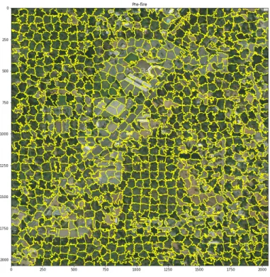
4.3.2.1 Converting pixels to objects via image segmentation: While taking advantage of WorldView-3’s high spatial resolution, image processing segmentation algorithms can be utilized to divide up an image into small areas. For converting the image into segments, the SLIC algorithm provided by scikit-image is used to cluster pixels by k-means on the 5-D Lab color space [7]. This segmentation step is only done on the Paradise pre-fire image.
Fig. 8: SLIC Image segmentation example on Paradise pre-fire image.
Prior to performing SLIC segmentation, the WorldView-3 image is split into 36 image chunks. Then, a select eight of the image chunks is segmented by SLIC with parameters n segmentsset to 5000 andcompactnessset to 10. Thecompactnessparameter controls the
color-similarity and proximity between segments andn segmentsinitializes the number of centers for k-means [7]. This results in a total of 14,086 segments that range in areas of approximately 750–2,300 square meters in size for each. Fig. 8 shows an example of SLIC segmentation breaking up a pre-fire image.
4.3.2.2 Vectorize image segments: Using rasterio and Shapely, each image segment is vectorized into a Polygon geometry and stored into a GeoDataFrame. This allows for quick indexing on the segment index when adding new features for the dataset. A preview of this GeoDataFrame is provided in Fig. 9.
Fig. 9: Preview of the intial GeoDataFrame.
4.3.2.3 Feature extraction: Digital numbers (DNs), spectral indices (SIs), and dSIs were extracted from the segments as features for the dataset. These features were selected as many burn severity classification algorithms have commonly used them to train their models as mentioned in Table 2. The steps for extracting features for the dataset is as follows.
1) Extract WorldView-3 band digital numbers:
For each segment, the mean digital numbers (DNs) are extracted by using Scikit-Image’sregionprops method and is stored into the GeoDataFrame. This is done for both the pre-fire and post-fire images of Paradise. A DN is the value of a pixel ranging from 0 to 255. DNs represent the reflected energy emitted from the ground [35]. 2) Extract Sentinel-2 band DNs with zonal statistics:
Because Sentinel-2 does not have the same spatial resolution as WorldView-3, the pixel sizes will differ in size and another method to extract the mean pixel value of a segment will be required. The zonal stats method in the rasterstats library is used to extract the mean value of the Sentinel-2 pre-fire and post-fire pixels within each segment. These values are also stored into the GeoDataFrame. Fig. 10 shows the overlapping vector of the segment on the Sentinel-2 image. Pixels highlighted in gray are selected and the mean pixel value is used as the new DN.
Fig. 10: Example of regionprops and zonal statistics.
3) Compute SIs:
Lastly, SIs and dSIs of the pre-fire and post-fire image segments are calculated by the Equations 1 and 2. A total of twelve SIs were created between all combinations of the image bands. This makes six SIs for the pre-fire image bands and six SIs for the post-fire image bands. Then six dSIs between the pre-fire and post-fire SIs were computed and stored into the GeoDataFrame as in Fig. 11.
Fig. 11: Preview of the complete GeoDataFrame.
4.3.3 Final Dataset
After completing the preprocessing and feature extraction steps, the GeoDataFrame is then downloaded as an ESRI Shapefile for manual labelling using ArcGIS Pro. This final dataset has a total of 14,086 samples and 26 features with two target classes:
• 8 bands:red, green, blue, near-infrared mean pixels. There are two VNIR bands for each pre-fire and post-fire segment. Their DNs are in the range [0, 255].
• 12 SIs: all combinations of spectral indices from the VNIR bands. For example, Green−Blue Green+Blue, Red−Green Red+Green, Red−Blue Red+Blue, NIR−Red
NIR+Red, etc. There are two for each pre-fire and post-fire segment. These SIs are based off of Equation 1 whereband1 has a higher wavelength than band2. These SIs range between [-1, 1].
• 6 dSIs:all changes between the SIs from their respective pre-fire and post-fire images as specified in Equation 2. dSIs range between [-2, 2].
• 1 burn class:this is the first target class where 1 represent a burned sample and 0 represents a non-burned sample.
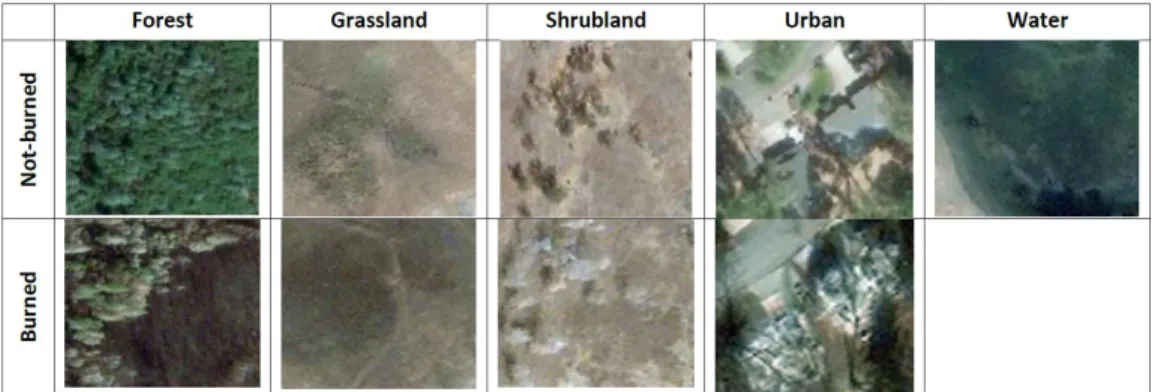
Fig. 12: Examples of land class. Photos from WorldView-3 of the Camp Fire.
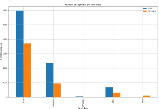
• 1 land class: this is the second target class with the following land-use classes. These classes are inspired by the concept of remote sensing’s land-use land-cover classification and California’s biomes [36]. Examples of each class are shown in Fig. 12. – Forest – Grassland – Shrubland – Urban – Water
(a) Number of samples in each class.
(b) Bar chart of number of segments per land class.
5 EXPERIMENTAL DESIGN 5.1 Experiment #1: Binary Classification
For the first experiment, a binary classification using the burn class label is performed on a variety of classification algorithms provided by the Scikit-Learn library. First, nine supervised learning algorithms will be compared in a stratified 10-fold cross-validation and using the results of each test after training. Then, the best model will be hypertuned by a 5-fold grid search. The dataset in this experiment is split into a train and test set of 67% and 33% respectively. The samples were stratified to ensure balance of the target class in both the train and test sets:
• Xtrain = 9,437 segments x 26 features • Xtest = 4,649 segments x 26 features
• ytrain= 6,056 burnt segments + 3,381 not-burnt segments • ytest = 2,983 burnt segments + 1,666 not-burnt segments
5.1.1 Cross-Validation
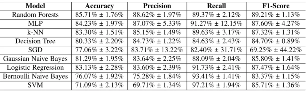
Nine base classifiers provided by the Scikit-Learn library are selected for cross-validation. These include random forests, logistic regression, Gaussian Naive Bayes, Bernoulli Naive Bayes, stochastic gradient descent (SGD), k-nearest neighbors (k-NN), decision trees, support vector machines (SVMs), and multi-layer perceptron (MLP) neural network. Then a stratified 10-fold cross-validation is performed on each model using the training dataset. Of these base models, only SVM’s n iter parameter is set to 10,000 iterations since training the SVM model had problems with convergence without limiting the iterations. Scikit-Learn’s SVM base model uses the radial basis function (RBF) kernel. The accuracy, precision, recall, and F1-score from the 10-fold cross-validation is provided with their 95% confidence intervals in Table 5 and is sorted by the descending precision score.
The top four algorithms with the highest precision are random forests, MLP, k-NN, and decision trees. These four models show good stability with low confidence intervals. Random forests has the best performance overall in accuracy, precision, and F1-score. SVM with the RBF kernel had the worst performance in accuracy and precision. SGD has volatile confidence intervals across all evaluation metrics and would not be considered reliable.
Table 5: Cross-Validation Results for Binary Classification
Model Accuracy Precision Recall F1-Score
Random Forests 85.71% ± 1.76% 88.62% ± 1.97% 89.37% ± 2.12% 89.21% ± 1.13% MLP 84.23% ± 1.97% 87.07% ± 5.33% 91.27% ± 12.15% 87.60% ± 4.27% k-NN 83.30% ± 1.51% 85.15% ± 1.49% 89.63% ± 3.17% 87.32% ± 1.31% Decision Tree 80.33% ± 2.20% 84.73% ± 1.22% 84.63% ± 2.43% 84.70% ± 0.89% SGD 77.06% ± 3.22% 83.71% ± 13.22% 82.40% ± 31.71% 69.25% ± 44.22% Gaussian Naive Bayes 81.29% ± 1.95% 83.64% ± 2.25% 88.09% ± 2.04% 85.80% ± 1.41%
Logistic Regression 83.13% ± 2.28% 83.60% ± 2.39% 91.73% ± 2.41% 87.47% ± 1.64% Bernoulli Naive Bayes 76.07% ± 1.92% 75.28% ± 1.84% 93.41% ± 1.41% 83.37% ± 1.15% SVM 71.09% ± 2.13% 69.71% ± 1.34% 97.21% ± 1.94% 85.71% ± 1.36%
5.1.2 Evaluation
After cross-validation, the remaining test dataset resulted in the evaluation scores shown in Table 6 on page 39. Although not reported previously in the cross-validation, the evaluation scores are also provided for SVMs trained with the linear and polynomial kernel. Each of the model’s confusion matrices are shown in Fig. 23, 24, and 25 in Appendix A.1. All of the classifiers had correctly predicted 83%–97% of the burnt segments. However, only random forests, MLP, k-NN, and the decision tree models had accurately predicted 73%–78% of the non-burned segments. Of these models, random forests has the best accuracy and precision scores of 85.65% and 88.32% respectively. Only second to random forests, MLP also has high accuracy and precision scores of 84.94% and 88.24% respectively. SVM with the RBF kernel has the worst in performance with an accuracy of 71.67%. However, SVM improves to 82.79% with the linear kernel and 85.31% with the polynomial kernel.
Table 6: Binary Classification Evaluation Scores
Model Accuracy Precision Recall F1-Score
Random Forests 85.65% 88.32% 89.47% 88.89%
MLP 84.94% 88.24% 88.30% 88.27%
k-NN 83.54% 85.05% 90.21% 87.55%
Decision Tree 80.38% 85.16% 84.08% 84.62%
SGD 77.26% 81.43% 83.64% 82.52%
Gaussian Naive Bayes 80.43% 82.24% 88.64% 85.32% Logistic Regression 83.20% 83.12% 92.62% 87.62% Bernoulli Naive Bayes 75.26% 74.67% 92.99% 82.83% SVM with RBF 71.67% 70.22% 96.98% 81.46% SVM with linear 82.79% 82.23% 93.36% 87.44% SVM with polynomial 85.31% 85.94% 92.19% 88.95%
5.1.3 Hyperparameter tuning
As it is determined from the evaluation that the random forest model has the best predictability on the binary burn class, the random forest base model parameters from Scikit-Learn are hypertuned. The steps described in this section are inspired by Koehrsen’s [37] hyperparameter tuning methods by using the best parameter ranges from the random search and then applying them to the exhaustive grid search. Using the same train and test dataset, a stratified 5-fold cross-validation splitting strategy is used for both random and grid search. First, a random selection of 25 parameters are chosen for the random grid search with the following parameter grid:
Listing 1: Random search parameter grid
1 {‘n_estimators’: [10, 114, 219, 324, 428, 533, 638, 743, 847, 952, 1057, 1162, 1266, 1371, 1476, 1581, 1685, 1790, 1895, 2000],
2 ‘max_features’: [‘auto’, ‘sqrt’, ‘log2’],
3 ‘max_depth’: [10, 19, 28, 37, 46, 55, 64, 73, 82, 91, 100, None],
4 ‘min_samples_split’: [2, 5, 10, 15, 100], 5 ‘min_samples_leaf’: [1, 2, 5, 10],
Then, a new parameter grid is hand-selected by the best parameter sets from the random search with precision scores of more than 80%. The exhaustive grid search is performed on 480 possible combinations of parameters from the following grid in Listing 2:
Listing 2: Grid search parameter grid 1 {‘n_estimators’: [200, 650, 1100, 1550, 2000], 2 ‘max_features’: [‘auto’, ‘sqrt’],
3 ‘max_depth’: [55, 70, 80, 90], 4 ‘min_samples_split’: [5, 10], 5 ‘min_samples_leaf’: [1, 2, 5], 6 ‘bootstrap’: [True, False]}
After the grid search, the random forest model with the highest precision score is selected with the best parameters as follows in Listing 3:
Listing 3: Best parameters from grid search {‘bootstrap’: False, ‘max_depth’: 55,
‘max_features’: ‘sqrt’, ‘min_samples_leaf’: 2, ‘min_samples_split’: 5, ‘n_estimators’: 200}
The best random forest model had an accuracy of 87.4% (+/- 1.2%), a precision score of 88.6% 1.0%), a recall score of 92.3% 1.0%), and a F1 score of 90.4% (+/-0.9%). Fig. 14 shows the improvements of the evaluation scores from the base models to the models selected by the random and exhaustive grid search. The selected random forests model from the grid search improved in accuracy by +1.75% from the base model.
5.2 Experiment #2: Multi-class Classification
In the second experiment, multi-class classification using both the burn class and land class is performed on Scikit-Learn classification algorithms like in Chapter 5.1. The target values are label encoded from the combination of both the burn class and land class starting from 0–8. The dataset is then split 67% for training and 33% for the test and is stratified. The training set contains 9,437 segments with 26 features and the test set has 4,649 segments with 26 features. Fig. 15 shows the number of samples that are in each train and test set.
Fig. 14: Random and grid search results for binary classification.
5.2.1 Cross-Validation
Similarly to Chapter 5.1, this experiment uses the same nine base classifiers from Scikit-Learn. Table 7 shows the results from multi-class classification on each model using a stratified 10-fold cross-validation. The evaluation metrics used in this experiment are overall accuracy, weighted precision, weighted recall, and weighted F1-score.
Like the binary classification results in Chapter 5.1, random forests remains the top algorithm with an accuracy of 77.14% and a weighted precision of 76.45%. MLP and k-NN also remain in the top three. SGD, SVM with the RBF kernel, and Bernoulli Naive Bayes has the worst performance across all metrics.
Table 7: Cross-Validation Results for Multi-class Classification
Model Accuracy Precision Recall F1-Score
Random Forests 77.14% ± 2.72% 76.45% ± 3.74% 77.35% ± 3.18% 76.47% ± 3.11% MLP 74.97% ± 3.58% 74.67% ± 3.47% 74.12% ± 3.07% 72.73% ± 3.44% k-NN 72.96% ± 2.90% 72.30% ± 2.98% 72.96% ± 2.90% 72.41% ± 2.91% Gaussian Naive Bayes 64.28% ± 2.00% 70.69% ± 1.51% 64.28% ± 2.00% 65.92% ± 1.68% Decision Tree 69.52% ± 3.23% 69.45% ± 2.68% 69.55% ± 3.21% 69.62% ± 2.65% Logistic Regression 71.51% ± 2.42% 67.55% ± 2.92% 71.51% ± 2.42% 68.81% ± 2.36% SGD 53.88% ± 22.54% 65.58% ± 15.00% 60.65% ± 9.54% 50.15% ± 22.64% SVM 56.42% ± 1.39% 65.14% ± 3.40% 56.42% ± 1.39% 50.73% ± 1.87% Bernoulli Naive Bayes 61.15% ± 2.82% 57.03% ± 4.37% 61.15% ± 2.82% 56.49% ± 2.54%
5.2.2 Evaluation
In Table 8 on page 43, overall accuracy, weighted precision, weighted recall, and weighted F1-score are reported for testing the models. The corresponding confusion matrices in Appendix A.2 are normalized to show the predictions made for the nine classes. It can be observed that random forests, MLP, k-NN, and decision trees were able to have some good predictions on the forest, grassland, and water classes. From the results given in Table 8 on page 43, random forests has the highest overall accuracy and weighted precision scores of 78.25% and 77.56% respectively. All of the SVM models had the worst performance with overall accuracies between 25.17%–57.28%. Random forests accurately predicted 81.7% of the non-burned forest segments and 85.8% burned segments as shown in Fig. 26(a) on page 67. 83.9% of the water segments were accurate. For the grassland land class, random forests had classified 76.4% of the burnt segments correctly, however, not burnt had only 56.1% correct. Lastly, for the urban land class random forests had predicted 51.1% as burned and 29.3% as not burned.
Table 8: Multi-class Classification Evaluation Scores Model Overall Accuracy Weighted Precision Weighted Recall Weighted F1-Score Random Forests 78.25% 77.56% 77.82% 77.17% MLP 77.44% 74.01% 74.45% 73.47% k-NN 73.39% 72.66% 73.39% 72.85% Decision Tree 70.51% 70.42% 70.51% 70.45% SGD 70.25% 67.28% 70.25% 67.47%
Gaussian Naive Bayes 64.68% 72.07% 64.68% 66.64% Logistic Regression 73.33% 69.25% 73.31% 70.72% Bernoulli Naive Bayes 63.17% 57.44% 63.17% 58.38%
SVM with RBF 57.28% 65.27% 57.28% 52.10%
SVM with linear 38.72% 44.63% 38.72% 38.43%
SVM with poly 25.17% 41.70% 25.17% 28.05%
5.2.3 Hyperparameter tuning
Since random forests proved to have the best performance, similarly to Chapter 5.1, the random forests base model from Scikit-Learn are hypertuned using random search and grid search. Listing 1 on page 39 provides the random grid parameters in which 25 sets of parameters will be randomly selected. Then, the top hand-picked parameters with weighted precision scores above 80% from the random search produces the following parameter grid in Listing 4:
Listing 4: Grid search parameter grid 1 {‘n_estimators’: [325, 518, 712, 906, 1100], 2 ‘max_features’: [‘auto’, ‘log2’],
3 ‘max_depth’: [55, 65, 80, None], 4 ‘min_samples_split’: [2, 10], 5 ‘min_samples_leaf’: [1],
6 ‘bootstrap’: [True, False]}
Listing 5: Best parameters from grid search {‘bootstrap’: False, ‘max_depth’: 80,
‘max_features’: ‘auto’, ‘min_samples_leaf’: 1, ‘min_samples_split’: 2, ‘n_estimators’: 906}
The best model selected after the exhaustive grid search had an overall accuracy of 79.5% 1.0%), weighted precision of 79% 1.2%), weighted recall of 79.5% (+/-1.0%), and a weighted F1-score of 79% (+/- 1.0%). In Fig. 16, it can be seen that the overall accuracy of the random forest model improved by +1.25% from the base model after the grid search.
5.3 Experiment #3: Multi-class Classification with Spark
For the last experiment, the validity of using Spark MLLib for burn severity classifica-tion is explored. Because Spark datasets like Resilient Distributed Datasets (RDDs) are of a different data structure than NumPy and pandas, some preprocessing is required in order to transform the current dataset into a format that is suitable for Spark. For MLLib, it requires the use of a file format called LIBSVM that represents a labelled sparse feature vector:
label index1:value1: index2:value2 index3:value3...