présentée devant
L’Université de Rennes 1 Spécialité : informatique
par
Thomas Genet
Reachability analysis of rewriting for
software verification
soutenue le 30 novembre 2009 devant le jury composé de :
M. Olivier Ridoux Président MM Ahmed Bouajjani Rapporteurs
John Gallagher Michael Rusinowitch
MM Hubert Comon-Lundh Examinateurs Thomas Jensen
Je remercie Ahmed Bouajjani, John Gallagher et Michael Rusinowitch de s’être penchés sur ce travail et d’avoir accepté d’en être les rapporteurs. Dans la mesure où ce travail tente de combiner certaines caractéristiques du model-checking régulier et de l’analyse statique par interprétation abstraite dans un outil de preuve basé sur la réécriture, il était naturel que je vous demande d’en être les rapporteurs. Cependant, je vous remercie d’avoir accepté ensemblede vous acquitter de cette tâche. Vos retours respectifs me seront précieux. Je remercie, en plus, John d’avoir fait l’effort de venir depuis Roskilde même s’il a, au change, gagné quelques degrés et quelques heures de soleil!
Je remercie Hubert Comon-Lundh de participer au jury. C’est, pour moi, un peu un retour aux sources car, si je me souviens bien, j’ai présenté les premiers balbutiements de ces travaux pendant un séminaire que tu organisais. Tu m’avais d’ailleurs gentiment indiqué de précieuses références, notamment celles des travaux de Florent Jacquemard, que j’avais complètement manquées. Merci, donc, d’apporter à ce jury ton expertise dans le domaine des automates d’arbres et des systèmes de réécriture ainsi que dans le domaine de la vérification des protocoles cryptographiques qui est un des nombreux violons d’Ingres que tu partages avec Michael.
Je suis très heureux qu’Olivier Ridoux soit dans ce jury. Tout d’abord parce que, Olivier, je suis fan de ton esprit curieux et inventif (et je ne suis pas le seul). Une sec-onde raison est que je pense que la soutenance sera l’occasion pour toi de me poser des questions qui risquent de me tarabuster pendant quelques temps. Enfin, j’espérais pou-voir m’enorgueillir d’apou-voir le seul président de jury en chemise hawaïenne. Cependant, il semble que tes mandats de directeur de l’IFSIC et bientôt de l’ESIR aient eu raison de ta garde-robe, à mon grand désespoir (à nouveau, je ne suis pas le seul).
Un grand merci à Thomas Jensen d’avoir constamment (mais délicatement!) oeuvré pour que je rédige ce document et soutienne cette habilitation. Merci aussi, Thomas, de m’avoir fait profiter de ta vision de l’interprétation abstraite afin de guider mes tentatives de rapprochement avec les approximations régulières en réécriture. D’autre part, je profite de l’occasion pour te remercier de ton accueil chaleureux dans l’équipe Lande (maintenant Celtique). Pendant toutes ces années, notamment en co-encadrant des doctorants, j’ai tenté de saisir la Jensen’s touch: rigueur et fermeté, le tout enrobé d’une grande dose d’humanité. J’espère pouvoir, à mon tour, utiliser et transmettre cet enseignement. Merci également d’avoirinsistépour participer au jury, ça fait toujours plaisir.
Je remercie tous mes collègues de l’IRISA et de l’IFSIC qui contribuent à faire de ces deux instituts des endroits où il fait bon vivre, travailler et enseigner. Il n’est pas possible de remercier nominativement tout le monde. Je pense, en particulier, à mes nombreux collègues de l’IFSIC. Merci à tous pour votre bonne humeur, cela aide à se lever le matin.
A l’IRISA, je peux difficilement ne pas remercier Lydie Mabil qui sait anticiper, quand il en est encore temps, ou résoudre, quand il est trop tard, tous nos problèmes, gros et petits. Le tout dans la bonne humeur. Chapeau. Merci aussi à tous mes collègues des équipes Celtique, Lis et Vertecs pour les discussions impromptues, les séminaires au vert et les, irremplaçables, pauses du midi.
Je remercie, particulièrement, mes anciens voisins de bureau: Michael Périn, Frédéric Besson, David Pichardie, Olivier Heen et maintenant David Cachera pour leur patience. Pas toujours facile de partager un bureau avec un batteur compulsif, désolé.
Je remercie Vlad Rusu pour sa curiosité, sa ténacité et son talent. J’espère que notre collaboration, initiée à l’occasion d’un des articles couvert par ce document, se poursuivra. Je remercie Olivier Heen de s’être intéressé à ces travaux même si ceux-ci ne sont pas toujours très “sécu”. Merci aussi pour cette passionnante collaboration autour de la valori-sation des outils de vérification de protocoles cryptographiques pour Thomson R&D. Je me dois, aussi, de remercier Francis Klay avec qui j’ai fait mes premières armes sur ce sujet à France Telecom avant d’être recruté à l’IRISA.
Je remercie mes trois doctorants: Valérie Viet Triem Tong, Luka Le Roux et Benoît Boyer d’avoir essuyé les plâtres. J’espère qu’ils n’auront pas trop de séquelles après dé-moulage. Merci aussi à Guillaume Feuillade dont j’ai eu la chance d’encadrer le stage de DEA. J’espère, simplement, qu’on arrivera un jour à finir ce fichu papier sur la complé-tude. Merci à tous les membres de l’ANR RAVAJ d’avoir cru et contribué à ce projet. La façon dont cela s’est passé donne presque envie de re-signer! Dans cette équipe, un merci tout particulier à Yohan Boichut pour sa participation efficace et motivante à la plupart des sujets abordés dans ce document. Et, ça ne va sans doute pas s’arrêter là. Merci également à Axel Legay pour nos discussions préliminaires, avec Benoît Boyer, sur la vérification de propriétés temporelles sur les automates d’arbres. De toutes façons, je sais très bien que s’il n’est pas remercié il va faire la gueule.
Cette longue liste seraient incomplète si elle n’incluait pas Isabelle Puaut qui a genti-ment accepté de faire six mois supplégenti-mentaires en tant que responsable du master 1 afin de me permettre d’achever, dans de bonnes conditions, ma période de délégation et ce docu-ment. Isabelle, je sais que tu étais vraiment prête à tout pour trouver un remplaçant, mais sache que j’apprécie ton geste!
Enfin, je souhaite remercier ma famille pour son soutien indéfectible, même s’ils ne savent pas vraiment ce que je fais et que je pourrais tout aussi bien construire des bag-noles à La Janais. Je remercie de tout coeur Valérie qui m’a soutenu pendant toutes ces années bien qu’elle sache, elle, effectivement à quoi je passe mes journées. Merci aussi à Maxime, Sarah et Lou pour leur énergie communicative et, en même temps, pour leur compréhension, leur patience et leur calme quand papa travaille à la maison.
1 Preliminaries 9
2 State of the art 13
2.1 Term rewriting systems preserving the regularity . . . 13
2.1.1 Known classes of the literature . . . 13
2.1.2 The FPO and GFPO criteria and algorithm . . . 16
2.1.3 The L-IOSLT algorithm . . . 19
2.2 Approximations of reachable terms . . . 19
2.2.1 Equational abstraction . . . 19
2.2.2 Inferring equational abstractions on tree automata . . . 21
2.3 Other analysis with tree abstract domains . . . 21
2.3.1 Analysis of tree transducers . . . 21
2.3.2 Analysis of imperative, functional and logic programs using regu-lar languages . . . 24
3 Theoretical contributions 31 3.1 The standard Tree Automata Completion algorithm . . . 31
3.1.1 The standard critical pair solving . . . 32
3.1.2 Normalization rules . . . 37
3.1.3 The exact case . . . 37
3.1.4 Extension to the conditional case . . . 45
3.2 Equational Tree Automata Completion . . . 49
3.2.1 Simplification of Tree Automata by Equations . . . 49
3.2.2 R/E-coherent Tree Automata . . . 53
3.2.3 One step of equational completion . . . 58
3.2.4 The full Completion Algorithm . . . 63
3.3 Comparison with other work . . . 68
3.3.1 Recognizing regular classes with standard completion . . . 68
3.3.2 Recognizing regular classes with equational completion . . . 72
3.3.3 Equational abstraction . . . 74
3.3.4 Regular and abstract regular tree model-checking . . . 76
3.3.5 Static Analysis . . . 77 3
4 Practical contributions 83
4.1 TheTimbuklibrary . . . 83
4.1.1 History . . . 83
4.1.2 Timbuktree automata completion and reachability analysis tool . . 85
4.1.3 Taml . . . 93
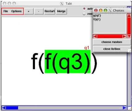
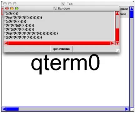
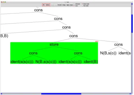
4.1.4 Tabi . . . 96
4.1.5 Known users . . . 98
4.2 Tree automata matching optimization . . . 99
4.2.1 Basic matching algorithm . . . 99
4.2.2 An optimized algorithm for epsilon-free automata . . . 101
4.2.3 Dealing with epsilon transitions and matching . . . 104
4.3 Implementation and use of matching inTimbuk . . . 106
4.3.1 Tabling and propagation of new substitutions . . . 106
4.3.2 Simplification of tree automata with equations . . . 108
4.4 Tree automata completion extensions . . . 108
4.4.1 Discussion about non left-linear term rewriting systems . . . 108
4.4.2 Restricted conditional term rewriting systems . . . 112
4.5 Tree automata completion checker . . . 114
4.6 Comparison with other tools . . . 115
4.6.1 On regular classes . . . 116
4.6.2 Other tree automata completion tools . . . 118
4.6.3 Completion as an alternative for breadth-first search . . . 120
4.6.4 Equational abstraction with Maude . . . 122
5 Applications 127 5.1 Cryptographic protocol verification . . . 127
5.1.1 The problem . . . 127
5.1.2 Encoding into TRS and verification by tree automata completion . . 129
5.1.3 The SmartRight case study . . . 131
5.1.4 Comparison with other tools . . . 136
5.2 Prototyping of static analyzers . . . 136
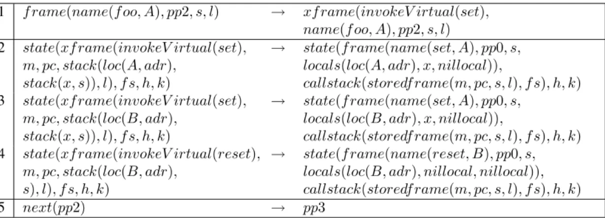
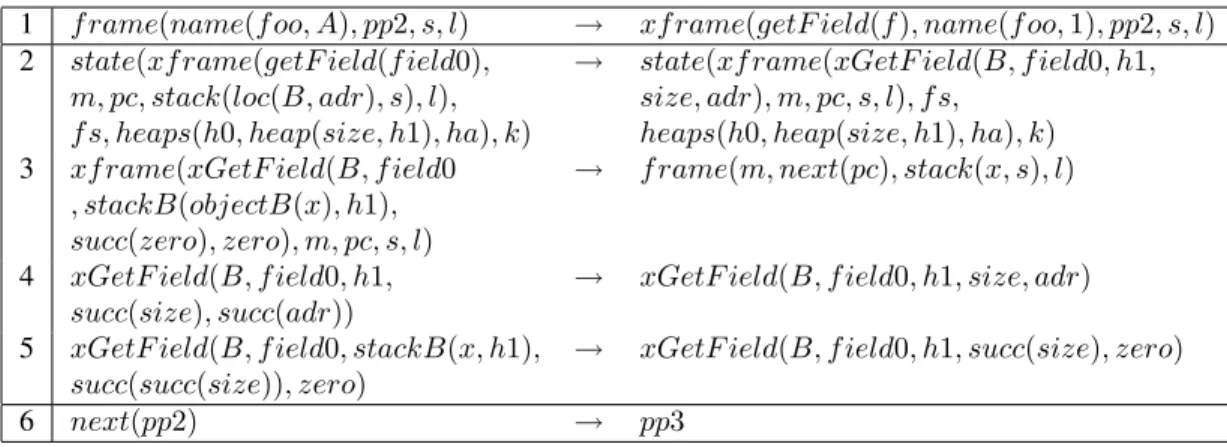
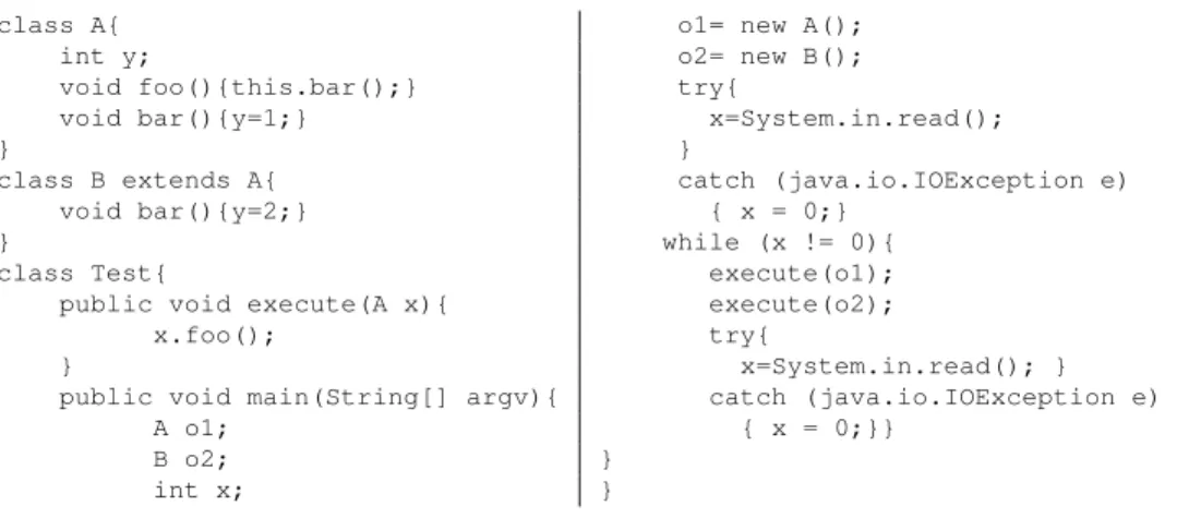
5.2.1 Translation of Java Bytecode Semantics into TRS . . . 138
5.2.2 Analysis in the single threaded case . . . 144
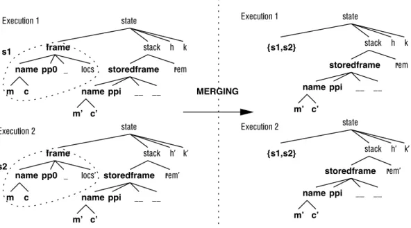
5.2.3 Analysis of multi-threaded programs . . . 147
5.2.4 Copster . . . 149
5.3 Proof of strong non termination . . . 150
6 Conclusion 153
This work is concerned with software verification techniques, i.e. how to prove proper-ties on softwares. The techniques we focus on do not require to execute the program. These techniques are commonly qualified asstatic in opposition todynamic techniques like testing that require to run the program. Static techniques prove properties on a model of the program built either from its code or from its specification.Model-checkingproves a temporal property on a program specification that is a specific model of a program. This technique is based on the exploration of the graph of reachable program states which needs to be finite or, at least, have a finite description. Static analysisbuilds an abstraction of the program from its source code and then proves properties on this model. These models, obtained usingabstract interpretation, permit to prove properties on infinite sets of reach-able program states. However, if the abstraction is too coarse, static analysis is not abble to prove the expected property. Besides to these techniques, the complete specification and verification can be performed using aproof assistant. In that case, the logic embedded in the proof assistant is usually expressive enough to specify the program and prove the expected property. However, the proof is generally done by hand with few automatic steps. In the domain of static analysis and model-checking, verification techniques have to be fully automatic. Hence, a verification technique needing additional information, provided by a human, to succeed is not considered as reasonable. On the opposite, in the domain of user-assisted proof, a verification technique that fails to prove a property and that cannot be guided so as to finish one particular proof is frustrating. Our objective is to propose a verification technique in between. On the one side, the technique we propose is based on abstractions so as to handle infinite models. On the other side, when abstractions are too coarse and proof fails, our technique permits to guide the verification by hand using approximation refinement.
A verification framework based on rewriting
For the verification technique to be as general purpose as possible, the formalism needs to be simple and expressive enough for modeling heterogeneous software systems. This is the reason why we use Term Rewriting Systems (TRS for short) to model programs. TRS are used for automated deduction for more than 40 years. More recently, they have been used for program modeling. TRS are particularly well suited for this purpose and they can model in a simple and readable way a large variety of computational systems. For instance, TRS can model deduction systems, functions, parallel processes or transition systems for
which rewriting respectively models: deduction, evaluation, progression or transitions. In addition, rewriting makes it also possible to model any combination of them, for instance: two processes executing functional programs or, as shown in Section 5.2.1, several threads executing Java programs. Finally, another interest of the rewriting framework is that it can be used to model programs either at high level of abstraction, e.g. a specification, or at low level, e.g. machine code. Cryptographic protocols are an example of a high level specification modeled in an abstract way using TRS. Messages are represented using terms and dynamics of the protocol using TRS. Rewriting models the reaction of each agent when receiving a specific message, i.e. rewrite rules are of the form “on reception of this message, I send this message”. Though it is simple, this model is enough to perform very deep and efficient verifications (Armando et al., 2005; Genet and Klay, 2000) and to come up with tricky attacks on classical cryptographic protocols of the literature (Chevalier and Vigneron, 2002) and even on industrial protocols under development (Heen et al., 2008). By opposition to those high level models, we also use rewriting to model the execution of Java at the lowest level, i.e. at the bytecode level (Boichut et al., 2007). In this case, terms encode the Java Virtual Machine (JVM) state and rewriting represents the execution of each bytecode instruction of the program.
The core verification technique: proving (un)-reachability
on rewriting
In the field of rewriting, the reachability problem is well-known: given a term rewriting systemRand two ground termssandt,tis said to beR-reachable from theinitialterms (denoted bys→R∗t) ifscan be rewritten intotwith a finite number ofRrewriting steps.
On the opposition,tisR-unreachable froms(denoted bys6→R∗ t) if there exists no way
to rewritesintot.
Reachability and unreachability proofs can be used as general purpose verification tech-niques for the systems modeled using rewriting. For deduction systems, functions, parallel processes, transition systems, proving unreachability will respectively show that a property cannot be deduced, a function call cannot be evaluated into a forbidden value, that a critical configuration (like a deadlock) will never happen, or that a state is unreachable from the initial configuration. On the two above examples: cryptographic protocols and Java byte-code, an unreachability proof can ensure that a security protocol does not leak a secret or that the execution of a given Java program never puts the JVM in a forbidden state.
All the contributions presented in this document are related to software verification using (un)reachability proofs on term rewriting systems. When the TRSRis terminating and the set of initial termssis finite, the problem is decidable. Indeed, to decide ifs→R∗t
it is enough to rewritesbyR, in all possible ways, and check if it can be rewritten into t. Since Ris terminating, the rewriting tree is finite and so is its exploration. This is close to a naive model-checking algorithm using exploration of the model. The situation is different whenRis not terminating or when the set of initial term is not finite. For instance, TRSs used for the verification of security protocols are not terminating (See Section 5.1). One of the reasons for that is that the TRS encodes an unbounded number of successive
protocol sessions. For Java program verification, though the TRS encoding the execution of a program may terminate, it is uneasy to show it because it is huge. Besides to this, the objective is generally to prove the safety of the program for any set of entries, i.e. an unbounded number of initial termss.
In those two situations, a finite exploration of the rewriting tree is impossible. However, under some syntactic restrictions onR(detailed in Section 2.1.1), for a given set of initial termsL, theset of reachable termsR∗(L) ={t |s∈ L ∧ s→R∗ t}can be computed.
SinceRmay not be terminating andLmay not be finite,R∗(L)is not necessarily finite.
Infinite sets of terms are usually finitely represented using tree automata. Thus, given a tree automaton recognizing the setLand for some classes of TRSR, the setR∗(L)is
recognized by a tree automatonBand the reachability problem becomes decidable. Indeed, deciding ifBrecognizestis easy and it is equivalent to deciding ift∈ R∗(L).
Nevertheless, as we will see in Section 2.1.1, syntactical classes for which there ex-ists an automaton recognizing exactly R∗(L) are very restrictive and few TRSs mod-eling real programs fall into those classes. For general TRS, it is possible to build an over-approximationApproxofR∗(L)and thus give a criterion for unreachability only:
s6→R∗tifs∈ Landt6∈App.
Contributions
This document surveys our main contributions to the proof of (un)reachability on term rewriting systems as well as two applications. Our first contribution concerns the preci-sion of the tree automata completion algorithm proposed in (Genet, 1998) whose role is to build an automatonApproover-approximatingR∗(L). We show that, underexact
nor-malizing strategy, this algorithm computes exactly the set of reachable terms for many interesting TRS classes. This is the case for most of the linear TRS classes for which the set of reachable terms is known to be regular: Ground TRS (Dauchet and Tison, 1990; Brainerd, 1969), Linear and Semi-Monadic (Coquidé et al., 1991), Linear and (inversely) Growing (Jacquemard, 1996), Linear Generalized Semi-Monadic (Gyenizse and Vágvöl-gyi, 1998), Linear Path Overlapping (Takai et al., 2000), Linear Generalized Finite-Path Overlapping (Takai, 2004), Constructor Based (Réty, 1999). As a corollary, our results provide simpler proofs of regularity for those classes. Furthermore, since the tree automata completion algorithm was initially designed to build over-approximations, thesame al-gorithm can do both. Thus, tree automata completion computes reachable terms exactly when the TRS belongs to one of the above classes and permits to over-approximate them otherwise.
The second contribution is to have proposed and integrated in the completion proce-dure two languages for defining approximations: normalization rules and approximation equations. Normalization rules are an ad-hoc language that mimics the structure of the completed tree automaton. As a result, this language lets the user fully adapt the approxi-mation to its verification objective. However, since it is a low-level language, the precision of the approximations defined using normalization rules is difficult to estimate. This is the reason why we propose another language, approximation equations, whose semantics is formal and is based on equivalence classes. Using this language makes it possible to prove
a second precision result which is that any automaton produced by completion with a set of approximation equations recognizes no more than terms reachable by rewriting modulo the set of equations.
While the above results tend to refine the precision of completion and the precision of approximations, we also worked on extending its scope. A third contribution is to have extended the tree automata completion to the case of conditional term rewriting systems. Using conditions significantly improves the expressiveness of the language used to model the systems to verify and can lead to shorter specifications.
The fourth contribution is the implementation of all the above results in a tool. This tool,Timbuk, permits to compute exactly the automaton recognizing the set of reachable terms when possible and to build an over-approximation using normalization rules or equa-tions, otherwise. This part is particularly concerned with the optimization of several of the algorithms used in tree automata completion.
The last contribution, is to have applied reachability analysis usingTimbukon realistic verification problems, namely verification of cryptographic protocol and static analysis of Java bytecode programs. For cryptographic protocols, our work was one of the first to over-approximate the execution of a protocol in an unbounded Dolev-Yao model, i.e. unbounded number of protocol sessions, unbounded number of agents and unbounded number of sym-bolic intruder actions. This approach was then refined so as to deal with an industrial copy-protection protocol designed by Thomson R&D. For Java bytecode verification, our objective was to show that tree automata completion is an interesting way of fast prototyp-ing and fine tunprototyp-ing static analysis to a particular property to prove. Finally, since all the above analysis rely on a similar model, i.e. a completed tree automaton, they can all be certified using acommonfixpoint checker. In particular, this checker is independent of the program to verify, the property to prove and the precision of the approximation.
Outline of the document
Chapter 1 gives some definitions and notations necessary to read the document. Then, in Chapter 2, we present a survey of known classes of TRS for which the set of reachable termsR∗(L)is known to be computable exactly whenLis recognized by a tree
automa-ton. In the same chapter, we also survey works closely related to over-approximation of reachable terms. In Chapter 3, we propose our algorithm calledtree automata comple-tionas well as the two languages we use to define approximations: normalization rules and equations. In this chapter, we show that completion without any approximation, com-putes exactlyR∗(L)for left-linear TRSs falling into the decidable classes of Section 2.1.1.
Given a set of approximation equationsE, we show a precision result saying that com-pletion computes no more thanR/E-reachable terms, i.e. terms that can be reached by rewriting initial terms withRmoduloE. At the end of the chapter, we draw some compar-ison with other techniques for exact and approximated computations ofR∗(L)presented
in Chapter 2. Chapter 4, presentsTimbukas well as some other tools designed to experi-ment with tree automata and tree automata completion. Finally, Chapter 5 details our two main case studies of reachability analysis on TRS using tree automata completion, namely cryptographic protocol verification and Java bytecode verification.
Preliminaries
Comprehensive surveys can be found in (Dershowitz and Jouannaud, 1990; Baader and Nipkow, 1998) for term rewriting systems, and in (Comon et al., 2008; Gilleron and Tison, 1995) for tree automata and tree language theory.
Definition 1 (Terms,T(F)andT(F,X)) LetF be a finite set of symbols, each associ-ated with an arity, and letX be a countable set of variables. T(F,X)denotes the set of terms, andT(F)denotes the set of ground terms (terms without variables). Definition 2 (Term variables,Var(t)) The set of variables of a termtis denoted byVar(t).
Definition 3 (Substitution) A substitution is a functionσ fromX intoT(F,X), which can be extended uniquely to an endomorphism ofT(F,X). Definition 4 (Term position) A positionpfor a termtis a word overN. The empty
se-quencedenotes the top-most position. The setPos(t)of positions of a termtis inductively defined by:
• Pos(t) ={}ift∈ X
• Pos(f(t1, . . . , tn)) ={} ∪ {i.p|1≤i≤nandp∈ Pos(ti)}.
Definition 5 (Subterm at positionp,t|p) Ifp∈ Pos(t), thent|pdenotes the subterm oft
at positionp.
Definition 6 (Term replacement,t[s]p) t[s]pdenotes the term obtained by replacement of
the subtermt|pat positionpby the terms.
Definition 7 (Multiple term replacement,t[pi←ti|1≤i≤m]) Let t be a term and
p1, . . . , pm be positions of t such that pi and pj are disjoint if i 6= j. The
replace-ment in t of subterms of t at positions p1, . . . , pm with terms t1, . . . , tm is denoted by
t[pi←ti|1≤i≤m]
Definition 8 (Ground context,C[ ]) A ground contextC[ ]is a term ofT(F ∪ {2}) con-taining exactly one occurrence of the symbol2. Ift ∈ T(F)thenC[t]denotes the term
obtained by the replacement of2bytinC[ ].
Definition 9 (Rewrite rule) A rewriting rule is a pair of terms(l, r)∈ T(F,X)×T(F,X), denoted byl→r, wherel6∈ X, andVar(l)⊇ Var(r). Definition 10 (Term Rewriting System, TRS) A term rewriting systemRis a set of rewrite
rules.
Definition 11 (Equation) An equation is a pair of terms(s, t) ∈ T(F,X)× T(F,X),
denoted bys=t.
Definition 12 (Linear terms) A term t is linear if each variable ofVar(t)occurs only
once int.
Definition 13 (Linear, Left-linear, Right-linear rewrite rule and TRS) A rewrite rulel→ risleft-linear(resp. right-linear) ifl(resp. r) is linear. A TRS is left-linear (resp. right-linear), if all its rewrite rules are left-linear (resp. right-linear). A rewrite rule (or a TRS)
islinearif it is left and right-linear.
Definition 14 (Linear equation and linear set of equations) An equations=tis linear ifsandtare linear. A set of equations is linear if all its equations are linear. Definition 15 (Rewrite relation,→R) Let Rbe a TRS andl → r a rewrite rule ofR.
Lets, t ∈ T(F). The termscan be rewritten intot, denoted bys→R t, if there exists a
positionp∈ Pos(s)and a substitutionσsuch thats|p=lσandt=s[rσ]p, i.e.
s=s[lσ]p→Rs[rσ]p=t
The reflexive transitive closure of→Ris denoted by→∗R.
Definition 16 (Termination ofR,→R) A term rewriting systemR, or the associated rewrite
relation→R, is said to be terminating if there is no infinite rewrite chains→Rs1→R. . .
Definition 17 (Normal form, irreducible term,IRR(R)) A terms ∈ T(F,X)is said to be in normal form or irreducible w.r.t. a TRSRif there exists no termt∈ T(F,X)such thats→Rt. The set of terms irreducible w.r.t.Ris denoted byIRR(R).
Definition 18 (Rewriting up to a normal form,→R!) A terms∈ T(F,X)can be
rewrit-ten into a normal formt ∈ T(F,X)if s →R∗ tand t ∈ IRR(R). This is denoted by
Definition 19 (Confluence ofR,→R) A term rewriting systemR, or the associated rewrite
relation→R, is said to be confluent if for all termss, t, u∈ T(F,X)such that
s R ∗ ∗ R ? ? ? ? ? ? ? ? t u
then there exists a termv∈ T(F,X)such that t R ∗ > > > > > > > > u ∗ R v Definition 20 (E-equivalence or equality moduloE) The E-equivalencerelation is de-fined as follows.
• First, for two ground termst, t0∈ T(F)and an equationl=r, we say thatt=t0if there exists a substitutionτ:X 7→ T(F)such thatlτ =tandrτ =t0;
• Then, we define the equivalence relation=E⊆ T(F)× T(F)as the smallest
con-gruence containing the relation{(t, t0)∈ T(F)× T(F)|t=t0}.
Definition 21 (E-equivalence class or quotient of a set of terms by a set of equationsE) Thequotient of the setL ⊆ T(F)by a set of equationsE, denoted byL/E, is the set of sets of terms defined as follows.
• Fort∈ T(F),[t]Edenotes the=E-equivalence class oft;
• Then,L/E={[t]E|t∈ L}.
Definition 22 (←→E) For any set of equationsE,←→E ={l→r, r→l|l=r∈E}. Definition 23 (R-descendants,R∗(L)) The set ofR-descendants of a term setL ⊆ T(F)
isR∗(L) = {t ∈ T(F)| ∃s ∈ Ls.t.s →∗
R t}. We extend this notation to terms in the
following way:R∗(s) =R∗({s}).
Definition 24 (R-normal forms,R!(L)) The set of R-normal forms of a term setL ⊆ T(F)isR!(L) =R∗(L)∩IRR(R).
Definition 25 (Equational rewriting, rewriting modulo a set of equations) Given a TRS R, a set of equationsEand two termss, t∈ T(F),s→R/Et⇐⇒ ∃s0, t0∈ T(F)s.t.s=E
The relation→∗
R/Eis the reflexive transitive closure of→R/E.
Definition 26 (R/E-descendants) The set of R/E-descendants of a language of terms L ⊆ T(F)isR∗
E(L) ={t∈ T(F)| ∃s∈ Ls.t.s→∗R/E t}.
The verification technique we propose in this paper is based on the computation of R∗(L). Note thatR∗(L)is possibly infinite:Rmay not terminate and/orLmay be infinite. The set R∗(L) is generally not computable (Gilleron and Tison, 1995). However, it is
possible to over-approximate it (Feuillade et al., 2004; Takai, 2004) using tree automata, i.e. a finite representation of infinite (regular) sets of terms. We next define tree automata.
Let Q be a finite set of symbols, with arity0, called states such that Q ∩ F = ∅. T(F ∪ Q)is called the set ofconfigurations.
Definition 27 (Transition, normalized transitions and epsilon transitions) Atransition is a rewrite rulec → q, where cis a configuration i.e. c ∈ T(F ∪ Q)andq ∈ Q. A normalized transitionis a transitionc → qwherec = f(q1, . . . , qn),f ∈ F ann-ary
symbol, andq1, . . . , qn∈ Q. Anepsilon transitionc→qis such thatc∈ Q.
Definition 28 (Bottom-up non-deterministic finite tree automaton (NFTA)) A bottom-up non-deterministic finite tree automaton (tree automaton for short) is a quadrbottom-upleA=
hF,Q,Qf,∆i, whereQf ⊆ Qand∆is a set of normalized transitions and epsilon
tran-sitions.
The rewriting relation on T(F ∪ Q) induced by the transitions ofA (the set ∆) is denoted by→∆. When∆is clear from the context,→∆will also be denoted by→A.
Definition 29 (Recognized language) The tree language recognized by A in a state q is L(A, q) = {t ∈ T(F) | t →∗
A q}. The language recognized by A is L(A) = S
q∈QfL(A, q). A tree language is regular if and only if it can be recognized by a tree
automaton.
Example 30 (Tree automaton and recognized language) Let F = {f, g, a} and A =
hF,Q,Qf,∆i, whereQ={q0, q1, q2, q3, q4},Qf={q0}, and∆ ={f(q1)→q0, g(q1, q1)→
q1, a→q1}. The languages recognized byq1andq0are the following:L(A, q1)is the set of terms built on{g, a}, i.e.L(A, q1) =T({g, a}), andL(A, q0) =L(A) ={f(x)|x∈ L(A, q1)}.
We also define epsilon and epsilon-free derivations which are necessary both for com-pletion and simplification of tree automaton by equation application.
Definition 31 (epsilon and epsilon-free derivations) We denote by→ rewritings performed by epsilon transitions. Conversely we denote bys →6A t (resp. s →6∆ t) the fact that s→At(resp.s→∆t) and no epsilon transition has been used for rewriting.
State of the art
In this chapter, we review some of the papers where regular languages are used to compute or over-approximate the semantics of a TRS, tree transducer or more generally of a pro-gram. The first section is devoted to the computation of the image of a regular language by a TRS. We first review the known classes of TRS for which the image of a regular lan-guage is regular. These classes are also known asclasses of TRS preserving the regularity. Then, we also review some papers dealing with regular over-approximations of the image. In Section 2.3, we present some other papers not dealing with TRS but which are also us-ing regular languages to model the semantics of tree transducers, functional programs and imperative programs.
2.1
Term rewriting systems preserving the regularity
2.1.1
Known classes of the literature
The basic reachability problem we are going to consider is the following: given a term rewriting systemRand two termss, t ∈ T(F), can we decide whethers →?
R tor not?
In this part, we focus on the existing solutions designed for particular cases. The simplest case is whenRis terminating. Here is a simple but inefficient procedure: to decide whether s→R?tor not it is enough to see ift∈ R∗(s)sinceR∗(s)is finite and computable.
WhenRis not terminating, deciding reachability needs some additional formal tools. For instance, tree automata can be used to finitely represent the infinite setR∗(s) and
then check ift ∈ R∗(s). Many works are devoted to the construction ofR∗(S)for a
regular languageS and a term rewriting systemR. The setR∗(S)is clearly not always
regular, choose for instanceS = {f(a, b)}andR= {f(x, y) → f(s(x), s(y)). In this case,R∗(S) ={f(sn(a), sn(b))| n∈
N}. In fact, it was shown in (Gilleron and Tison,
1995) that deciding whetherR∗(S)was regular is not possible in general, even ifRis a
confluent and terminating linear TRS. Thus, most of the results define classes of TRSR so thatR∗(S)is regular. First, we present the classes which can be defined with simple
syntactic restrictions onR:
G: Ris a ground TRS (Dauchet and Tison, 1990; Brainerd, 1969).
RL-M: Ris a right-linear and monadic TRS (Salomaa, 1988), i.e. right-hand sides of the rules ofRare either variables or terms of the formf(x1, . . . , xn)wheref ∈ Fand
x1, . . . , xnare variables.
L-SM: Ris a linear and semi-monadic TRS (Coquidé et al., 1991), i.e. rules are linear and their right-hand sides are of the formf(t1, . . . , tn)wheref ∈ Fand∀i= 1, . . . , n,
tiis either a variable or a ground term.
L-G−1: In (Jacquemard, 1996), Jacquemard defines the classL-Gof linear “growing” TRS, where “growing” means that every left-hand side is either a variable, or a term f(t1, . . . , tn)wheref ∈ F,Ar(f) =n, and for alli = 1, . . . , nthe termtiis a
variable, a ground term, or a term whose variables do not occur in the right-hand side. Jacquemard also shows that if Ris growing then (R−1)∗(S) was regular.
Those classes are essentially used for needness analysis of redex in rewriting, see for instance (Durand and Middeldorp, 1997). In order to compare this class with all the others onR∗(S), we can define theL-G−1class using the restrictions in the other direction. TheL-G−1 class corresponds to linear TRS where theright-hand side is either a variable, or a termf(t1, . . . , tn)wheref ∈ F,Ar(f) = n, and for all
i= 1, . . . , nthe termtiis a variable, a ground term, or a term whose variables do not
occur in theleft-hand side. Thus, note that in this class the usual variable restriction on rewrite rules, i.e.Var(l)⊇ Var(r)does not hold.
RL-G−1: similar toL-G−1except that left-linearity is not required. This result was proved by Nagaya and Toyama in (Nagaya and Toyama, 1999).
L-IOSLT: Ris a linear I/O separated layered transducing TRS (Seki et al., 2002). Those TRS are defined on sets of symbolsFi,Fo andP such that∀p∈P0 :Ar(g) = 1
andFi,FoandPare disjoint. Symbols ofFiare input symbols and those ofFoare
output symbols. In the TRS, all the rewrite rules are of the form: • fi(p1(x1), . . . , pn(xn))→p(to), or
• p0
1(x1)→p0(t0o)
wherefi ∈ Fi,p1, . . . , pn, p, p01, p0 ∈P,x1, . . . , xn are disjoint variables,to, t0o ∈
T(Fo,X) such thatVar(to) ⊆ {x1, . . . , xn} and Var(t0o) ⊆ {x1}. This class
corresponds to linear tree transducers as explained in section 2.3.1.
Recently, new and more general classes were found. The classes ofL-GSMlinear general-ized semi-monadic TRS (Gyenizse and Vágvölgyi, 1998),RL-FPOright-linear and finite-path overlapping TRS,L-FPOlinear finite-path overlapping TRS (Takai et al., 2000) and L-GFPOlinear generalized finite-path overlapping TRS (Takai, 2004). The regularity cri-teria used in classesL-GSM,RL-FPO,L-FPOandL-GFPOare more sophisticated and cannot be expressed as a simple syntactic restriction like above classes. They are based on a careful inspection of the syntactic structure of rewrite rules so that recursive application of rewrite rules are guaranteed to preserve regularity. We give some details on theRL-FPO andRL-GFPOcriteria in Section 2.1.2. Thanks to some results of (Takai et al., 2000) and
in (Takai, 2004), the expressiveness of all the above mentioned classes can be ordered in the following way.
Proposition 32 (Expressiveness of TRS classes) G RL-M L-SM L-G−1 y y rrrrrr rrrr RL-G−1 L-GSM L-FPO x x qqqqqq qqqq RL-FPO L-GFPO
and L-IOSLT is incomparable with others.
P. Réty (Réty, 1999) proposed another way of considering the problem and defined a class where restrictions are weaker on the TRS and stronger on the regular language S. Since this class imposes restrictions on the languageS it is thus incomparable with previous ones. We call this classconstructor based. The alphabetFis separated into a set ofdefined symbolsD={f | ∃l→r∈ Rs.t.Root(l) =f}and constructor symbols C = F \ D. The restriction on S is the following: S is the set of ground constructor instances of a linear termt, i.e.S={tσ}wheret∈ T(F,X)is linear andσ:X 7→ T(C). The restrictions onRare the following: for each rulel→r
1. ris linear, and
2. for each positionp∈ PosF(r)such thatr|p = f(t1, . . . , tn)andf ∈ Dwe have
that for alli= 1. . . n,tiis a variable or a ground term, and
3. there is no nested function symbols inr
Finally, some works also consider the construction of sets of reachable terms under classical evaluation strategies of rewriting or modulo theory. Réty and Vuotto have shown in (Réty and Vuotto, 2002) thatR∗(S)is still regular, with the same restriction as (Réty,
1999) onRandS, when rules ofRare applied under some specific strategies: innermost, outermost, . . . In (Bouajjani and Touili, 2005), Bouajjani and Touili show that the set of reachable terms for subclasses of Process Rewrite Systems (Mayr, 1998) can be computed exactly. Process Rewrite Systems can be seen as a particular case of TRS modulo the associativity, commutativity and neutrality of some symbols.
2.1.2
The FPO and GFPO criteria and algorithm
As seen above, RL-FPOandL-GPFOare some of the most general classes of TRSR such thatR∗(S)is regular ifS is. We now detail the FPO and GFPO criteria which are
based on the notion ofsticking-out. Roughly a termssticks out of a termtif they have in common a positionpsuch that (1) all symbols encountered on the path fromtopare the same insandt, and (2)t|pis a variable ands|pis either a variable or a non ground term.
This is formally defined as follows (Takai et al., 2000).
Definition 33 A termssticks-outof a termtat positionpwithp∈ PosX(t)\ {}if
• ∀o:o≺p∧o∈ Pos(s) =⇒ s(o) =t(o), and • p∈ Pos(s)ands|p 6∈ T(F).
Additionally, a termsproperly sticks-outof a termtat positionpits|pis not a variable.
Example 34 Assume that F = {f, g, a, b} andX = {x, y, z, u}. The termf(x, g(b))
sticks out of termf(y, a)at position1.andf(f(a, x), y)properly sticks-out off(z, g(u))
at position1..
Definition 35 (Sticking-out graph) Thesticking-out graphof a TRSRis a directed graph G = (V, E)whereV = R, the vertices are the rules ofR, and the setE is defined as follows. Letv1andv2be, possibly identical, vertices which corresponds to rewrite rules l1 →r1andl2→r2respectively. For i=1,2, replace each variable inVar(ri)\ Var(li)
by a fresh constant symbol.
1. Ifr2properly sticks-out of a subterm ofl1, thenE contains an edge fromv2 tov1 with weight one.
2. If a subterm ofr2properly sticks-out ofl1, thenE contains an edge fromv2 tov1 with weight one.
3. If a subterm ofl1sticks-out ofr2, thenEcontains an edge fromv2tov1with weight zero.
4. Ifl1sticks-out of a subterm ofr2, thenEcontains an edge fromv2tov1with weight zero.
Example 36 LetF ={f, g, a, b},X ={x, y}andR={p1=f(x, a)→f(h(y), x), p2=
g(y)→f(g(y), b)where fori= 1,2li(resp.ri) denotes the left (resp. right)-hand side of
pi. Sinceyoccurs inr1but not inl1it is replaced by theconstant. Sincer2=f(g(y), b)
properly sticks out off(x, a)at position1., inEwe have an edge betweenp2andp1of weight1. Then, sincel2 = g(y)sticks-out ofr2 = f(g(y), b)at position1., inE we have an cyclic edge of weight0on p2. Note that there is no cyclic edge onp1 because r1=f(h(), x)does not sticks-out ofl1 =f(x, a)at position1.becauser1|1.=h()
p1 p2
0 1
Definition 37 A TRS is Finite Path Overlapping (FPO) if its sticking-out graph has no
cycle of weight1or more.
Theorem 38 (RL-FPO TRS preserve regularity (Takai et al., 2000)) IfSis a regular lan-guageSandRis a right-linear FPO (RL-FPO) TRS thenR∗(S)is regular.
When dealing with linear TRS, the criterion can be improved as shown in (Takai, 2004). It is based on the notion ofGeneralized sticking-out graphwe now define.
Definition 39 (Generalized sticking-out graph) Thegeneralized sticking-out graphof a TRSRis a directed graphG = (V, E). The setV of vertices is defined byV = {(l → r, x)|l→r∈ Randx∈ Var(l)∪ Var(r)}. The setEof edges is defined as follows. Let l1→r1andl2→r2be two rules ofR, possibly identical.
1. Ifr2properly sticks-out at positionpofl1|p0 withp0∈ Pos(l1), then fory=l1|p.p0 and for all variablesx∈ Var(r2|p),Econtains edges from(l2 →r2, x)to(l1 →
r1, y)with weight one.
2. Ifl1|p0 withp0 ∈ Pos(l1)sticks-out ofr2at positionp, then forx=r2|pand for all variablesy∈ Var(l1|p.p0),Econtains edges from(l2→r2, x)to(l1→r1, y)with weight zero.
3. Ifr2|p0 withp0 ∈ Pos(r2)properly sticks-out ofl1at positionp, then fory =l1|p and for all variables x ∈ Var(r2|p.p0), E contains edges from(l2 → r2, x) to
(l1→r1, y)with weight one.
4. Ifl1sticks-out ofr2|p0 at positionp, then forx=r2|p.p0 and for all variablesy ∈ Var(l1|p),Econtains edges from(l2→r2, x)to(l1→r1, y)with weight zero.
Example 40 Let R = {h(f(x, h(g(y)))) → f(g(k(y)), h(x))},l = h(f(x, h(g(y))))
andr =f(g(k(y)), h(x)). Withp0 = 1., we have thatl|1. =f(x, h(g(y)))(properly)
sticks-out ofr=f(g(k(y)), h(x))at positionp= 2.1.. We are in the second case of the previous definition. We thus get that there are edges betweenr|p =xand all variables of
l|p0.pwhich is the set{y}. Hence we have an edge between(l →r, x)and(l →r, y)of weight0. Symmetrically, still withp0 = 1.,r =f(g(k(y)), h(x))properly sticks-out of
l|p0 =f(x, h(g(y)))at positionp= 1.. This corresponds to the first case of the previous definition. Hence, there are edges between all variables ofVar(r|p) ={y}andx=l|p0.p. Thus, there is an edge between(l→r, y)and(l→r, x)of weight1. Here is the complete generalized sticking-out graph:
(l→r, x) (l→r, y)
0 1
Definition 41 A TRS is Generalized Finite Path Overlapping (GFPO) if its generalized sticking-out graph has no cycle of weight1or more. Theorem 42 (L-GFPO TRS preserve regularity (Takai, 2004)) IfSis a regular language SandRis a linear GFPO (L-GFPO) TRS thenR∗(S)is regular.
Theorem 43 (Expressiveness of GFPO (Takai, 2004)) L-GFPO⊃L-FPO
We now present the algorithm used to construct the automaton recognizing R∗(S)
whenRis inL−GF P O. The algorithms proposed in (Takai et al., 2000) and (Takai, 2004) are very similar. In fact, on linear TRS they are exactly the same. We chose to detail the one forL−GF P Obecause it is simpler and shows the main common idea of both algorithms which is the notion ofpacked state(named structured state in (Takai, 2004)). Definition 44 (Packed state (Takai et al., 2000) and Packed automaton) For a set of sym-bolsFand a set of statesQ, the set of packed states, denoted byPF,Q, is defined by:
• ifq∈ Qthen{q} ∈ PF,Q, and
• ifF ∈ F,Ar(f) =nandp1, . . . , pn∈ PF,Qthen{f(p1, . . . , pn)} ∈ PF,Q, and
• ifp1, p2∈ PF,Qthenp1∪p2∈ PF,Q.
IfAis a tree automaton, thepacked automatonpack(A)is the tree automaton where, for all stateq∈ A, all occurrences ofqinQ, Qf,∆are replaced by{q}.
For readability, a packed state{p1, . . . , pn}is written ashp1, . . . , pni.
Example 45 LetF ={f, g}andQ ={q1, q2}. Here are some possible packed states of PF,Q:hq1i,hq1, q2i,hf(g(hq2i),hq1, q2i)i.
Then, the tree automata construction can be defined as follows using the procedure addtransandmodify.
Procedureaddtrans(t)This procedure takes a termtofT(F ∪ Q)as input and adds new packed states toQand new transitions to∆.
• ifhti ∈ Qthen do nothing;
• iftis a constant then add statehtitoQand transitiont→ htito∆;
• ift=f(t1, . . . , tn)then add transitionf(ht1i, . . . ,htni)→ htiand executeaddtrans(ti)
for all1≤i≤n.
Example 46 Assume thatQ={hqi}and∆ ={a→ hqi}. If we calladdtrans(f(hqi, f(a, b))), Qbecomes{hqi,hai,hbi,hf(hai,hbi)i,hf(hqi,hf(hai,hbi))i}and∆ = {a → hqi, a → hai, b→ hbi, f(hai,hbi)→ hf(hai,hbi)i, f(hqi,hf(hai,hbi))→ hf(hqi,hf(hai,hbi))i}.
Proceduremodify(A,R)
Input: tree automatonA=hF,Q,Qf,∆iand a linear TRSR.
Output: a tree automatonA0defined as follows.
For any rulel→r∈ R, any substitutionσ:X 7→ Qand any packed stateqsuch that lσ→A∗qandrσ6→A∗qthenA0is obtained fromAby adding the transitionhrσi →qto
Aand runningaddtrans(rσ).
Theorem 47 (Fixpoint ofmodify(Takai, 2004)) If there is a fixpoint automatonA∗ for
the equationX=modify(X,R)∪ AthenR∗(L(A)) =L(A ∗).
Note that this is very close to the tree automata completion algorithm defined in Sec-tions 3.1 and Section 3.2.
2.1.3
The L-IOSLT algorithm
For theL-IOSLTclass, we can define the algorithm using similar techniques, though it is not exactly the case in (Seki et al., 2002). We use again the packed states defined in the previous section and we define the followingmodifySLTprocedure.
ProceduremodifySLT(A,R)
Input: tree automatonA=hF,Q,Qf,∆iand a linearL-IOSLTTRSR.
Output: a tree automatonA0defined as follows.
For all substitutionσ : X 7→ Q, for all rewrite rulel →r ∈ R and all packed state q∈ Qsuch thatlσ→A∗qandrσ6→A∗q:
• ifl =f(p1(x1), . . . , pn(x1))→p(xi) = rwith(1≤ i≤n)thenA0 is obtained
fromAby addingp(xiσ)→qtoA;
• l=p01(x)→p0(x) =rthenA0is obtained fromAby addingp0(xσ)→qtoA;
• ifl = f(p1(x1), . . . , pn(x1)) → p(g(t1, . . . , tn)) = rthen A0 is obtained from
Aby adding the transitions g(ht1σi, . . .htnσi) → [q, p]and p([q, p]) → qto A
where[q, p]is a state made of the pairqandp., Then, we runaddtrans(t1σ), . . . , addtrans(tnσ);
• l=p01(x)→p0(g(t1, . . . , tn)) =rthenA0is obtained fromAby adding the
transi-tionsg(ht1σi, . . .htnσi)→[q, p0]andp0([q, p0])→qtoAand runningaddtrans(t1σ),
. . . ,addtrans(tnσ)
Theorem 48 (Fixpoint ofmodifySLT(Seki et al., 2002)) If R is aL-IOSLT TRS then there is a fixpoint automatonA∗for the equationX =modifySLT(X,R)∪AandR∗(L(A)) =
L(A∗).
2.2
Approximations of reachable terms
2.2.1
Equational abstraction
The papers (Meseguer et al., 2003, 2008) are not, strictly speaking, about computing a regular language approximating the semantics of a TRSR. However, the approximations
defined using, so-called, equational abstraction have much in common. In their framework, TRS are used to represent a transition relation between states encoded by terms. Properties are defined in Linear Temporal Logic (LTL) and verified using a model-checker that is implemented, using the rewriting logic, in Maude (Clavel et al., 2001). When the system has an infinite set of states, they propose to use a setEof equations to define equivalence classes of states. If this setEis well chosen, then the set of equivalence classes is finite and the corresponding approximation preserves the properties to prove. They show that it can help in proving safety properties, i.e. something bad will not happen. Their work go even further and show that, even with an over-approximation, it is possible to prove liveness properties, i.e. something good will finitely happen.
The framework Meseguer et al. defined is very generic and powerful. Conjointly to TRS, it also uses equations to state the axioms of the model. For simplicity, we chose here to focus on a restricted part of their framework where the system isonlydefined using a TRSR(with no axioms). Moreover, we only consider simple safety properties encoded bys 6→R∗ t wheres andt are terms encoding, respectively, an initial state and a bad
state. This is simpler than their framework, but the core problem is still there: sinceRmay rewrite infinitelys, how prove thats 6→R∗ t? They propose to define a set of equations
E, show thats6→∗
R/E tand use the fact that→R⊆→R/Eto prove thats6→R∗ t. Under
certain conditions, even ifRinfinitely rewritess,s6→∗
R/E tmay be finitely proven. This
is the case if the setR∗
E(s)contains only a finite set ofE-equivalence classes and no one
containst.
However, provings6→∗
R/Etusing only rewriting and a tool like Maude is not easy.
In-deed, for rewriting withR/Ethe equational part ofEis generally encoded using rewriting. More precisely,Eis oriented into another TRSR0terminating and ground confluent. IfR0
enjoys those two properties, equality moduloEbecomes decidable. For two ground terms sandt,s =E t iff there exists a termusuch thats →!R0 uandt →!R0 u. Let→R(R0) be the relation→R(R0)=→∗
R0 ◦ →R ◦ →∗R0. SinceR0 has been obtained by orienting equations ofE, ifs→∗
R(R0) tthens→∗R/E t. However the implication does not always hold in the opposite direction.
Example 49 ((Viry, 2002)) LetR={f(x+y)→g(x) +g(y)}andE ={x+ 0 =x}. Equations ofEcan be oriented intoR0 ={x+ 0→x}which is terminating and ground
confluent. We can prove thatf(0 + 0) + 0→∗
R/E g(0) +g(0)becausef(0 + 0) + 0→R
g(0) +g(0) + 0→R0 g(0) +g(0). However,f(x)cannot be rewritten by→R(R0)though f(x)→R/E g(x) +g(0)sincef(x) =Ef(x+ 0)→Rg(x) +g(0).
Having→R(R0)⊆→R/E and not →R(R0)⊇→R/E is a problem for verifying safety properties using equational abstractions. Indeed, the only provable facts with a rewriting tool like Maude are of the forms6→∗
R(R0)tthat do not always entails6→∗R/E t. For this inclusion to be true in the opposite direction, the coherence (Viry, 2002) property has to be proven onRandR0. Roughly,RandR0are coherent if for all termsthat can be rewritten
intot1byR, on one side, and intot2byR0, on the other side, thent1can be rewritten by
s R // R0 t1 R0 ∗ t2 R∗ //u
This property cannot be shown in general but there exists a syntactic condition onRand R0, called local coherence, that implies coherence. This criterion is based on a standard
critical pair technique between the rules ofRand those R0. In (Meseguer et al., 2003,
2008), several examples show that finding a set of approximation equationsEthat can be oriented into a TRSR0 enjoying termination, ground confluence and coherence withR
is not an easy task. However, when it exists, it permits to prove both safety and liveness properties using only rewriting, and thus, in a very efficient way.
2.2.2
Inferring equational abstractions on tree automata
Additionally to theL-GFPOclass (see Section 2.1.1), (Takai, 2004) proposes over-approximate the set of reachable terms when it is not regular. It is defined as an extension of itsmodify procedure. The extension proposed is based on abstract interpretation (Cousot and Cousot, 1977) and consists to add a widening operation tomodify. The widening automatically infers approximation from the Generalized sticking-out graph (Section 2.1.2). The inferred widening can be seen as the application of an equation of the formC[C[x]] =C[x]where C[ ]can be any context. The algorithm automatically construct the widening. However, the form of the equation is fixed and cannot, thus, guarantee the existence of a fixpoint for modifyfor any left-linear TRS.
In particular, equations of the formC1[C2[x]] = C2[C1[x]] orC[x] = xcannot be found automatically nor manually added. When executing several steps ofmodify, if a widening position is found, i.e. there exists at least one repetition of a contextC[ ], then the widening adds an epsilon transition encoding the repetition ofC[ ]. This transition directly widens the language of the formC[C[. . .]] byC∗[. . .]. More precisely, assume that the tree automatonAis such thata→A∗ q1,C[q1]→A∗ q2and thatC[q2]→A∗ q3. We thus haveC[C[q2]] →A∗ q2. The widening detects the regularity and simply add the epsilon
transitionq3→q2. We thus obtain the looping derivationC[q2]→A∗q3→q2recognizing
any language of the formC[. . . C[a]. . .]intoq2.
2.3
Other analysis with tree abstract domains
2.3.1
Analysis of tree transducers
Tree transducers can be viewed as particular cases of TRS where rewriting is applied either bottom-up or top-down. Here, we consider linear bottom-up tree transducer (Gécseg and Steinby, 1984; Comon et al., 2008) that are defined as follows.
Definition 50 (Linear Tree Transducer) Let Fi be a set of input symbols, Fo a set of
∀q∈ Q:Ar(q) = 1. Alinear tree transducerT is a tuplehQ,Fi,Fo,Qf,∆iwhere∆is
a set of rewrite rules of the form: • f(q1(x1), . . . , qn(xn))→q(u), or
• q0(x1)→q00(u0)
wheref ∈ Fi,q1, . . . , qn, q, q0, q00∈ Q,x1, . . . , xnare disjoint variables,u, u0 ∈ T(Fo,X)
such thatVar(u)⊆ {x1, . . . , xn}andVar(u0)⊆ {x1}. A transducerT recognizes a regular relationRT ={(t, t0)∈ T(Fi)× T(Fo)|t→∗∆ q(t0)whereq ∈ Qf}. We can define the image of a language by a transducer as follows:
givenS ⊆ T(Fi),RT(S) ={t∈ T(Fo)|s∈ Sand(s, t)∈RT}.
Theorem 51 (Recognizability of image (Gécseg and Steinby, 1984; Comon et al., 2008)) Given a recognizable languageS and a linear tree transducerT, the setRT(S)is
recog-nizable.
In (Seki et al., 2002), Seki et al. proposed the classL-TLof linear layered transduc-ing TRS which encompasses tree transducers. However, for aL-TLTRSRregularity of R∗(S)is only ensured for the L-IOSLTclass defined in Section 2.1.1 and corresponds
exactly to linear tree transducers. In the definition of L-IOSLT TRS,Fi andFoare
sup-posed to be disjoint. This is not necessary in tree transducers because rewriting is nec-essarily performed bottom-up. For instance, if a tree transducer has a rule of the form f(q(x))→q(f(x))and thus rewritesf(q(a))intoq(f(a))no rewriting can be performed on the subtermf(a). This is not the case in generalL-TLTRS and this leads to non regular sets of reachable terms like it is shown in Example 5 of (Seki et al., 2002). However, with the restrictionFi∩ Fowe cannot have the rewriting rulef(q(x)) →q(f(x))becausef
cannot occur both in the left and right-hand side of the rule. This is a simple encoding of the bottom-up strategy used in tree transducers in the symbols used in rewriting.
Several works are consideringRegular Tree Model-Checkingof protocols defined using linear tree transducers. In this setting, the model-checking essentially consists in building the tree automaton representing any number of application of the tree transducer. This problem has been investigated for instance in (Bouajjani and Touili, 2002) and efficient implementations have been proposed in (Abdulla et al., 2005). The construction proposed in (Bouajjani and Touili, 2002) is not limited to tree transducers. They use a widening technique to compute exactly the set of terms reachable by repeated applications of a tree transducer on a regular set of terms. More precisely, ifRn
T is the combination ofRT n
times andAis a tree automaton, the objective is to compute another tree automatonA0
such thatL(A0) =R∗
T(L(A)) =
S
n≥0R
n
T(L(A)), i.e. the reflexive transitive closure of
RT onL(A). The proposed widening is based on the detection of regularities an the
hyper-graph encoding of the tree automaton. The first result is that this widening is exact. The second result is that it terminates for a specific class of TRS called Well-Oriented Systems WOS. This is due to the fact that the application of TRS of this class can be simulated by the application of a finite number of linear tree transducers. Using repeated applications of Theorem 51, it is thus possible to prove that this class preserve regularity. TheWOSclass can be defined as follows.
Definition 52 (Well-Oriented Systems (Bouajjani and Touili, 2002)) LetS=S0∪. . .∪ Sn be disjoint finite sets of symbols. An-phase well-oriented system overS is a set of
rewriting rules of the form:
b(a(x1, x2), c1(x3, x4)) → a(b0(x1, x2), c1(x3, x4)) a(b(x1, x2), c1(x3, x4)) → b0(a(x1, x2), c1(x3, x4)) a(b(x1, x2), c2(x3, x4)) → b0(a(x1, x2), a(x3, x4)) b(x1, x2) → d(x1, x2) b(a(x1, x2), c1(x3, x4)) → d(a(x1, x2), c1(x3, x4)) a(b(x1, x2), c1(x3, x4)) → a(d(x1, x2), c1(x3, x4)) b(a(x1, x2), c2(x3, x4)) → a(d(x1, x2), d(x3, x4))
as well as the symmetrical forms of these rules obtained by commuting the children, wherea, b0, c1∈Si+1,b, c2∈Si, andd∈Si+2, such that0≤i≤n−2.
TheWOSclass is incomparable withRL-FPO,L-GFPOandL-IOSLTclasses. This can be shown as follows:
WOS6⊆RL-FPO: let us construct the sticking-out graph of the first form of rules of WOS. Let l1 (resp. r1) be the left (resp. right) hand side of the rule. Sincer1 properly sticks-out of the subterma(x1, x2)ofl1, we have a cyclic edge of weight1 on this rule. Hence it is notRL-FPO.
RL-FPO6⊆WOS: non left linear TRS cannot be handled byWOS.
WOS6⊆L-GFPO: as above the generalized sticking-out graph of the first form of rules ofWOShas a cyclic edge of weight1. Letl1(resp.r1) be the left (resp. right) hand side of the rule. Sincer1properly sticks-out of the subterma(x1, x2)ofl1, we have a cyclic edge of weight1on the node labeled by(l1→r1, x1).
L-GFPO6⊆WOS: collapsing rules, i.e. rules of the formf(x1, . . . , xn) → xi are not
covered byWOS.
WOS6⊆L-IOSLT: let us have a look at the form of the two first rules of theWOSclass. In the left-hand sides,aappears at positionin the first rule and at position1.in the second one. This is impossible in theL-IOSLT(and even inL-LT) class where sets of symbols occurring at positionandi.in left-hand sides have to be disjoint. L-IOSLT6⊆WOS: inL-IOSLT, we can have rules of the formq(x) → q0(x)for all
symbolsq, q0 ∈ Q. InWOS, the only rules of that form areb(x
1, x2)→d(x1, x2) whereb ∈Si,d∈Si+2andSi∩Si+2 =∅. As a result,L-IOSLTcovers a sets of rules of the form{q(x)→q0(x), q0(x)→q(x)}that are not covered byWOS. When the exact value ofR∗T(S)cannot be finitely computed, the algorithm and widen-ing of (Bouajjani and Touili, 2002) does not terminate. This is why Bouajjani et al. pro-posed in (Bouajjani et al., 2006a) theAbstract Regular Tree Model-Checkingwhere over-approximations ofR∗T(S) are computed, so as to prove some unreachability properties. The paper defines two main abstraction functions which can be seen as equivalence rela-tions on states of the constructed tree automaton. One of the required property is that those
equivalence relations are of finite index, i.e. there is only a finite number of equivalence classes. This property forces the constructed tree automaton to have a finite number of states and thus a finite number of transitions. Hence, the construction of the iterated appli-cation of the tree transducer on the tree automaton is forced to terminate. Here are the two proposed equivalence relations:
• two states are equivalent if their recognized languages are equal for terms of height lesser or equal to a givenn;
• given a set of tree automata P = {P1, . . . , PN}, two states q1 andq2 of A are
equivalent if{Pi ∈P | L(Pi)∩ L(A, q1)6=∅}and{Pi∈P | L(Pi)∩ L(A, q2)6= ∅}are equal.
The authors also mention the fact that this last relation has good properties for abstrac-tion refinement. Assume that the approximaabstrac-tion relaabstrac-tion is too coarse because one of the automata ofP, sayPi, recognizes botht1andt2. Roughly, to refine the approximation, it
is enough to add two new tree automataPN+1andPN+2recognizing respectivelyt1and t2so that the new approximation will distinguish them. For instance, ift1is a valid reach-able term andt2is due to the over-approximation, this is a natural way to excludet2of the approximation. One of the results of (Bouajjani et al., 2006a) is a theorem guaranteeing that any spurious counter-example can be removed using this technique.
2.3.2
Analysis of imperative, functional and logic programs using
reg-ular languages
As mentioned in (Cousot and Cousot, 1995), the idea of using regular tree grammar for program analysis is due to (Jones and Muchnick, 1979; Jones, 1987; Jones and Andersen, 2007) following (Reynolds, 1969). Then it has been reformulated by (Heintze and Jaffar, 1990) asset based analysis. Note that, set based analysis does not produce regular lan-guages but set constraints. However, the mechanism and the obtained result is very similar to grammars obtained by (Jones, 1987), as it is mentioned in (Heintze, 1993).
We choose here to give a uniform description of the analysis techniques proposed in those papers. Though not all papers actually use them, our equivalent description uses set constraints. The program semantics is encoded into a generic setS of set constraints of the formx ⊇ f(x1, . . . , xn),x ⊇ y ∪z,x ⊇ y∩z, etc. defined on a set of variable
X ={x, y, z, x1, . . .}. Then, this set of constraints is solved by an algorithm producing a tree grammar over-approximating the solution ofS. Again, in all those the papers, the pre-sentation of the solution looks different but its semantics is equivalent. For an imperative program (Cousot and Cousot, 1995), variables ofXrepresent the variables of the program and a set constraint is associated to each program point. For logic programs (Heintze and Jaffar, 1990), eachoccurrenceof a variable of the program and each predicate symbol is as-sociated to a variable ofXand the clauses of the program are translated into set constraints. In particular, if a variable appears several times in the right-hand side of a clause, i.e. it is non linear, each occurrence is associated to a different variable ofX. Finally, for functional programs (Jones and Andersen, 2007), a variable ofX is associated to each parameter in function headers and the function definitions are translated into set constraints.
Though the construction of set constraints differs with programming paradigms, their resolution phases are very similar. The only difference is that constraints produced by functional and imperative programs do not contain any constraint of the formx⊇y∩z making the resolution far more easy. This is even mentioned by Heintze in (Heintze, 1993) as the main cause for performance problems of logic program analysis. He even advise to eliminate or limit as much as possible the use of intersection constraints for the modeling of logic programs. In the following, we do not consider intersection constraints.
The approximation used for the resolution of the constraints is similar in all the men-tioned papers. The intuition is the following: every set of tuples of the form{(a, b),(c, d)} is approximated by the set{(a, b),(a, d),(c, b),(c, d)}. In other words, the approximation forgets the relations between elements of a tuple in a set. This approximation is called “in-dependent attributes” in (Jones and Andersen, 2007). (Cousot and Cousot, 1995) propose some refinement of this approximation, based on a threshold for targeting the approxima-tion, but the general idea remains the same. Since the results of the resolution techniques are similar, we detail only one of them. We chose the analysis of (Jones, 1987; Jones and Andersen, 2007) because it translates functional programs into TRS and, thus, makes comparison with our techniques on TRS more accurate.
Example 53 Here is an example of a program, in ML-style, which is needing lazy evalua-tion to terminate. It is borrowed from (Jones and Andersen, 2007).
l e t r e c f i r s t l 1 l 2 = match l 1 , l 2 w i t h [ ] , _ −> [ ] | 1 : : m , x : : x s −> x : : ( f i r s t m x s ) l e t r e c s e q u e n c e y= y : : ( s e q u e n c e ( 1 : : y ) ) l e t g n= f i r s t n ( s e q u e n c e [ ] )
This program can be encoded into the following TRSRwhere ’one’ encodes ’1’, ’cons’ encodes ’::’ and ’nil’ encodes the empty list ’[]’.
f irst(nil, Xs)→nil
f irst(cons(one, M), cons(X, Xs))→cons(X, f irst(M, Xs))
sequence(Y)→cons(Y, sequence(cons(one, Y)))
g(N)→f irst(N, sequence(nil))
Note that, the obtained TRS is left-linear by construction because functional definitions are.
The algorithm described in (Jones, 1987; Jones and Andersen, 2007) propose to compute a tree grammar over-approximating the collecting semantics of the functiongfor a given set of inputs. It can be seen also as an over-approximation of the image of a set of inputs by a functiong. Informally, the grammar associates a non-terminalX to each variableX of the program and, for each function call, several non-terminalsRi to represent its set
of intermediate results. More precisely, if the functionf is defined usingkrewrite rules thenknon-terminals are associated to f. Note that, when there is no intersection, any
set constraints can be translated into a tree grammar rule and vice versa. For instance, a production of the form R0 →
G f(a) | R1 | R0 corresponds to the set constraintR0 ⊇
f(a, R2)∪R1∪R0with set of variables{R0, R1, R2}. A first step for the analysis of the program consists in building the grammar of the initial calls for which we want to analyze the program. On the previous TRS, a grammarGdescribing some interesting inputs can be:
R0 →
G g(Ω)
Ω →
G nil|cons(Atom,Ω)
Atom →
G zero|one| . . .
Then, the algorithm tries to match left-hand sides of rules ofRwith (subterms of) the right-hand sides of the productions ofG. For instance, the definition ofg(N)can be matched on g(Ω)with solution{N7→Ω}. In that case several productions and non-terminal are added to the grammar. First, since there is only one rewrite rule definingg, only one non-terminal, sayR1, is associated to any call ofg. In our case,R1 represents the set of intermediate results of the computation ofg(N)withN = Ω. Then, one non-terminal per parameter in the definition ofgis added, i.e. here only oneN. Finally the following productions relating the non-terminal to their values are added.
R0 →
G R1
R1 →
G f irst(N, sequence(nil))
N →
G Ω
The first production encodes the fact that every result ofR1 is also a result for R0, the second one unfolds the definition ofgand the last explicits the found match betweenN andΩ. Then, the algorithm continues onGcompleted with those productions. The next term to be replaced issequence(nil). Like forg, thesequencefunction is defined using1
rewrite rule. LetR4be the non-terminal associated to the calls of thesequencefunction. The left-hand side of the rule ofRdefining thesequencefunction i.e. sequence(Y)can be matched on the subtermsequence(nil)of the above productions leading to a solution {Y 7→nil}.
R1 →
G f irst(N, R4)
R4 →
G cons(Y, sequence(cons(one, Y)))
Y →
G nil
as before, the first production explicits the link that exists between intermediate results for R4 andR1. Then, matching betweensequence(Y)andsequence(cons(one, Y))gives the solution{Y 7→ cons(one, Y)}. Then, since thesequencefunction is associated to the unique non-terminal R4, the termsequence(cons(one, Y))is also replaced by R4. Note that this naturally leads to looping rules for non-terminalR4andY in the generated productions:
R4 →
G cons(Y, R4)
Y →
G cons(one, Y)