Bodo Rosenhahn1, Thomas Brox2, Daniel Cremers2, and Hans-Peter Seidel1 1Max Planck Center Saarbr¨ucken, Germany
[email protected] 2CVPR Group, University of Bonn, Germany
Abstract. Tracking 3D objects from 2D image data often leads to jittery tracking
results. In general, unsmooth motion is a sign of tracking errors, which, in the worst case, can cause the tracker to loose the tracked object. A straightforward remedy is to demand temporal consistency and to smooth the result. This is often done in form of a post-processing. In this paper, we present an approach for online smoothing in the scope of 3D human motion tracking. To this end, we extend an energy functional by a term that penalizes deviations from smoothness. It is shown experimentally that such online smoothing on pose parameters and joint angles leads to improved results and can even succeed in cases, where tracking without temporal consistency assumptions fails completely.
1
Introduction
Tracking 3D objects from 2D images is a well known task in computer vision with various approaches such as edge based techniques [8], particle filters [7], or region-based methods [14,1], just to name a few. Due to ambiguities in the image data, many tracking algorithms produce jittery results. On the other hand, smoothing assumptions of the observed motion can be made due to the inertness of the masses of involved objects. This means, that it is physically unlikely that an object continuously moved by a robot arm or human hand is rapidly changing the direction or even jittering, unless there are physiological diseases. Many tracking procedures do not take this property into account. Hence, the outcome tends to wobble around the true center of the tracked object. To receive a more appealing outcome, the results are often smoothed in a second post-processing step. However, jittery results often indicate errors or ambiguities during tracking. Thus, introducing temporal consistency already during the estimation, can help to eliminate errors at the root of the problem.
In case of human motion capturing and animation, several approaches exist in the literature to smooth motions of joints during synthesis. Bruderlin et al. [3] use a multi target motion interpolation with dynamic time warping in a signal based approach or Sul et al. [16] and Ude et al. [17] propose an extended Kalman filter. While these works have only addressed the smoothing of joint angles, the smoothing of 3D rigid body motions has been addressed in other works: Chaudhry et al. [6] smooth Euler angles and translation vectors. Shoemake [15] proposes quaternions for rotation animation (and interpolation) combined with translation vectors. Park et al. [12] use a rational
This work has been supported by the Max-Planck Center for Visual Computing and
Communication.
F.A. Hamprecht, C. Schn¨orr, and B. J¨ahne (Eds.): DAGM 2007, LNCS 4713, pp. 163–172, 2007. c
interpolating scheme for rotations by representing the group with Cayley parameters and using Euclidean methods in this parameter space. Belta et al. [4] propose a Lie-group and Lie-algebra representation in terms of an exponential mapping and twists to interpolate rigid body motions.
All these works concentrate on the synthesis, smoothing, and interpolation of given motion patterns, whereas in this work we smooth estimated motions online during a tracking procedure: we use a previously developed markerless motion capture system, which performs image segmentation and pose tracking of articulated 3D free-form sur-face models. In complex scenes (e.g. outdoor environments), we frequently observed the effect of motion jitter as a precursor to tracking failure. Therefore, in this work, we supplement a penalizer to the existing error functional in order to reduce large jit-ter effects. Whereas the penalizer jit-term for joint angles (as scalar functions) is pretty straightforward, the challenging aspect is to formalize penalizers for rigid body mo-tions. To achieve this, we use exponentials of twists to represent rigid body motions (RBMs) and a logarithm to determine from a given RBM the generating twist, simi-lar to the motion representation in [11,12]. The gradient of the penalizer leads to linear equations, which can easily be integrated in the numerical optimization scheme as addi-tional constraints. In several experiments in the field of markerless motion capture, we demonstrate the improvements obtained with the integrated smoothness assumptions. As we cannot give a complete overview on the vast variety of existing motion capture systems, we refer to the surveys [9,10].
2
Foundations
In this section, we introduce mathematical foundations needed for the motion penalizer, in particular the twist representation of a rigid body motion and the conversion from the twist to the group action as well as vice-versa. Both conversions are needed later in Section 4 for the smoothing of rigid body motions.
2.1 Rigid Body Motion and Its Exponential Form
Instead of using concatenated Euler angles and translation vectors, we use the twist representation of rigid body motions, which reads in exponential form [11]:
M=exp(θξˆ) =exp ˆ ω v 03×1 0 (1)
whereθξˆis the matrix representation of a twistξ ∈se(3) ={(v,ωˆ)|v∈R3,ωˆ∈so(3)}, with so(3) ={A∈R3×3|A=−AT}. The Lie algebra so(3)is the tangential space of all 3D rotations. Its elements are (scaled) rotation axes, which can either be represented as a 3D vector or a skew symmetric matrix:
θω=θ ⎛ ⎝ωω12 ω3 ⎞ ⎠,withω2=1 θωˆ=θ ⎛ ⎝ ω03 −0ω3−ωω21 −ω2 ω1 0 ⎞ ⎠. (2)
A twistξ contains six parameters and can be scaled toθξ for a unit vectorω. The pa-rameterθ∈Rcorresponds to the motion velocity (i.e., the rotation velocity and pitch).
For varyingθ, the motion can be identified as screw motion around an axis in space. The six twist components can either be represented as a 6D vector or as a 4×4 matrix:
θξ=θ(ω1,ω2,ω3,v1,v2,v3)T,ω2=1, θξˆ=θ ⎛ ⎜ ⎜ ⎝ 0 −ω3 ω2 v1 ω3 0 −ω1v2 −ω2 ω1 0 v3 0 0 0 0 ⎞ ⎟ ⎟ ⎠. (3)
se(3) to SE(3). To reconstruct a group action M∈SE(3)from a given twist, the ex-ponential function M=exp(θξˆ) =∑∞k=0(θk!ξˆ)k must be computed. This can be done efficiently via exp(θξˆ) = exp(θωˆ) (I−exp(θωˆ))(ω×v) +ωωTvθ 0 1 (4) and by applying the Rodriguez formula
exp(θωˆ) =I+ωˆsin(θ) +ω2(1−cos(θ)). (5) This means, the computation can be achieved by simple matrix operations and sine and cosine evaluations of real numbers. This property was exploited in [2] to compute the pose and kinematic chain configuration in an orthographic camera setup.
SE(3) to se(3). In [11], a constructive way is given to compute the twist which generates a given rigid body motion. Let R∈SO(3)be a rotation matrix and t∈R3a translation vector for the rigid body motion
M= R t 0 1 . (6)
For the case R=I, the twist is given by
θξ=θ(0,0,0, t
t), θ=t. (7)
In all other cases, the motion velocityθand the rotation axisωare given by
θ=cos−1 trace(R)−1 2 , ω= 1 2 sin(θ) ⎛ ⎝rr3213−−rr2331 r21−r12 ⎞ ⎠. To obtain v, the matrix
A= (I−exp(θωˆ))ωˆ+ωωTθ (8)
obtained from the Rodriguez formula (see Equation (4)) needs to be inverted and mul-tiplied with the translation vector t,
v=A−1t. (9)
This follows from the fact that the two matrices which comprise A have mutually orthogonal null spaces whenθ=0. Hence, Av=0⇔v=0. We call the transformation from SE(3)to se(3)the logarithm, log(M).
2.2 Kinematic Chains
Our models of articulated objects, e.g. humans, are represented in terms of free-form surfaces with embedded kinematic chains. A kinematic chain is modeled as the con-secutive evaluation of exponential functions, and twistsξiare used to model (known)
joint locations [11]. The transformation of a mesh point of the surface model is given as the consecutive application of the local rigid body motions involved in the motion of a certain limb:
Xi=exp(θξˆ)(exp(θ1ξˆ1). . .exp(θnξˆn))Xi. (10)
For abbreviation, we note a pose configuration by the(6+n)-D vectorχ= (ξ,θ1, . . . , θn) = (ξ,Θ)consisting of the 6 degrees of freedom for the rigid body motionξ and the nD vectorΘ comprising the joint angles. In the MoCap-setup, the vectorχis unknown and has to be determined from the image data.
2.3 Pose Estimation from Point Correspondences
Assuming an extracted image contour and the silhouette of the projected surface mesh, closest point correspondences between both contours can be used to define a set of corresponding 3D rays and 3D points. Then a 3D point-line based pose estimation al-gorithm for kinematic chains is applied to minimize the spatial distance between both contours: for point based pose estimation each line is modeled as a 3D Pl¨ucker line
Li= (ni,mi), with a unit direction ni and moment mi[11]. For pose estimation the
re-constructed Pl¨ucker lines are combined with the screw representation for rigid motions. Incidence of the transformed 3D point Xiwith the 3D ray Li= (ni,mi)can be expressed
as
(exp(θξˆ)Xi)3×1×ni−mi=0. (11)
Since exp(θξˆ)Xiis a 4D vector, the homogeneous component (which is 1) is neglected to evaluate the cross product with ni. This nonlinear equation system can be linearized in
the unknown twist parameters by using the first two elements of the sum representation of the exponential function:
exp(θξˆ) = ∞
∑
i=0 (θξˆ)i i ≈(I+θ ˆ ξ). (12)This approximation is used in (11) and leads to the linear equation system
((I+θξˆ)Xi)3×1×ni−mi=0. (13)
Gathering a sufficient amount of point correspondences and appending the single equa-tion systems, leads to an overdetermined linear system of equaequa-tions in the unknown pose parametersθξˆ. The least squares solution is used for reconstruction of the rigid body motion using Equation (4) and (5). Then the model points are transformed and a new linear system is built and solved until convergence. The final pose is given as the consecutive evaluation of all rigid body motions during iteration.
Since joints are expressed as special screws with no pitch of the form θjξˆj with
known ˆξj (the location of the rotation axes is part of the model) and unknown joint
angleθj. The constraint equation of an ith point on a jth joint has the form
(exp(θξˆ)exp(θ1ξˆ1). . .exp(θjξˆj)Xi)3×1×ni−mi=0 (14)
which is linearized in the same way as the rigid body motion itself. It leads to three linear equations with the six unknown twist parameters and j unknown joint angles.
3
Markerless Motion Capture
The motion capturing model we use in this work can be described by an energy func-tional, which is sought to be minimized [13]. It comprises a level set based segmenta-tion, similar to the Chan-Vese model [5], and a shape term that states the pose estimation task: E(Φ,p1,p2,χ) =− Ω H(Φ)log p1+ (1−H(Φ))log p2+ν|∇H(Φ)|dx segmentation +λ Ω(Φ−Φ0(χ)) 2dx shape error (15)
The functionΦ ∈Ω →Rserves as an implicit contour representation. It splits the image domainΩ into two regionsΩ1andΩ2withΦ(x)>0 if x∈Ω1andΦ(x)<0 if
x∈Ω2. Those two regions are accessible via the step function H(s), i.e., H(Φ(x)) =1 if x∈Ω1and H(Φ(x)) =0 otherwise. Probability densities p1 and p2measure the fit of an intensity value I(x)to the corresponding region. They are modeled by local Gaussian distributions [14]. The length term weighted byν>0 ensures the smoothness of the extracted contour.
By means of the contourΦ, the contour extraction and pose estimation problems are coupled. In particular, the projected surface modelΦ0acts as a shape prior to support the segmentation [14]. The influence of the shape prior on the segmentation is steered by the parameterλ=0.05.
Due to the nonlinearity of the optimization problem, an iterative minimization scheme is chosen: first the pose parametersχ are kept constant, while the functional is mini-mized with respect to the partitioning. Then the contour is kept constant, while the pose parameters are determined to fit the surface mesh to the silhouettes (Section 2.3).
4
Penalizing Motion Jitter
To avoid motion jitter, the idea is to extend the energy functional in (15) by an additional error term that penalizes deviations of the estimated pose from a smooth prediction generated from the poses of previous frames.
Such a predictionχ= (ξ,Θ)(as global pose) can be computed by means of the joint angle derivatives,
and the twist that represents the predicted position, ˆ
ξ =log
exp(ξˆt)exp(ξˆt−1)−1exp(ξˆt)
, (17)
see Section 2.1. The deviation of the estimateχ= (ξ,Θ)from the prediction can now be measured by ESmooth=|log exp(ξˆ)exp(ξˆ)−1 |2+|Θ−Θ|2. (18) Notice that the deviation of the rigid body motion is modeled by the minimal geodesics between the current and predicted pose.
This error value is motivated from the exponential form of rigid body motions: since we linearize the pose, see (13), we have to do exactly the same here. The derivative of the joint angles is simply given byΘ−Θ. To compute the motion derivative we can apply the logarithm from Section 2.1 to get a linearized geodesic [11]. This follows from the fact that the spatial velocity corresponding to a rigid motion generated by a screw action is precisely the velocity generated by the screw itself. To see this, we first set
exp(ξˆ):=exp(ξˆ)exp(ξˆ)−1, (19) withξ=log(exp(ξˆ)exp(ξˆ)−1). Let g(0)∈R3be a point transformed to
g(θ) =exp(ξˆθ)g(0). (20)
The spatial velocity of the point is given by [11] ˆ V=g˙(θ)g−1(θ). (21) Since, d dt(exp( ˆ ξθ)) =ξˆθexp(ξˆθ), (22) we have ˆ V =g˙(θ)g−1(θ) (23) =ξˆθ˙exp(ξˆθ)g(0)g−1(θ) (24) =ξˆθ˙g(θ)g−1(θ) =ξˆθ˙. (25) After setting ˙θ =1 (θ =t), the linearized penalizer term acts as additional linear
equation to the pose constraints which further regularize the equations, ∂ESmooth
∂ χ = (log(exp(ξˆ)exp(ξˆ)−1),Θ−Θ)=0. (26) Equation (26) yields an additional constraint for each parameter that draws the so-lution towards the prediction. Note that we do not perform an offline smoothing in a second processing step. Instead, the motion jitter is penalized online in the estimation procedure, which does not only improve the smoothness of the result, but also stabilizes the tracking.
5
Experiments
The experiments are subdivided into indoor and outdoor experiments. The indoor experiments allow for a controlled environment. The outdoor experiments demonstrate the applicability of our method to quite a tough task: markerless motion capture of highly dynamic sporting activities with non-controlled background, changing lighting conditions and full body models.
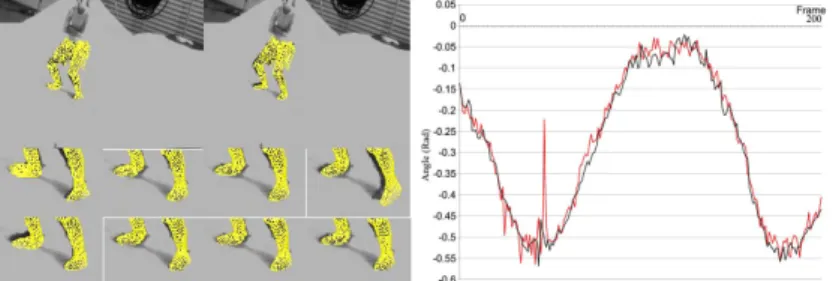
Fig. 1. Left: Example frames of a knee bending sequence. Right: Quantization of outcome: Red:
without penalizer, blue: with penalizer. The Penalizer function is suited to penalize rapid move-ment changes during tracking, not the smaller ones.
5.1 Indoor Experiments
For indoor experiments we use a parameterized mesh model of legs, represented as free-form surface patches.
Figure 1 shows in the left several consecutive example frames of a knee-bending scene in the lab environment. The smaller images in the first row show 4 example feet positions without a smoothness assumption and the last row shows feet positions with such an assumption. The motion jitter in these four consecutive frames is suppressed. The effect is quantified in the right of Figure 1. Here we have overlaid knee angles. The red values indicate the result of the system without the jitter penalizer and the blue one is the outcome with the incorporated penalizer. As can be seen, the penalizer decreases rapid motion changes, but maintains the smaller ones. The red peak around frame 50 is due to a corrupted frame, similar to the one in Figure 3
5.2 Outdoor Experiments
In our outdoor experiments we use two full body models of a male and female person with 26 degrees of freedom. Different sequences were captured in a four-camera setup (60 fps) with Basler gray-scale cameras. Here we report on a running trial and a coupled cartwheel flick-flack sequence, due to their high dynamics and complexity.
Figure 2 summarizes results of the running trial: all images have been disturbed by 15% uncorrelated noise and random rectangles of random color and size. Tracking is successful in both cases, with the smoothness assumption and without it. However,
Fig. 2. Running trial of a male person. Top: The images have been disturbed with uncorrelated
noise of 15% and random rectangles of random color and size. Bottom: Comparison of (some) joint angles: Red: Without jitter penalizer, black: with jitter penalizer. The curves reveal, that with the jitter penalizer the motion is much smoother.
Fig. 3. Tracking in an outdoor environment: corrupted frames can cause larger errors, which are
avoided by adding the penalizer function
the diagram reveals that the curves with a smoothness constraint are much smoother. A comparison with a hand-labeled marker-based tracking system revealed an average error of 5.8 degrees between our result and the marker-based result. More importantly,
Fig. 4. Red: Tracking fails, Blue: Tracking is successful
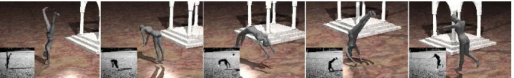
Fig. 5. Example frames of the (successful tracked) Cartwheel-Flick-Flack sequence in a virtual
environment. The small images show one of the four used cameras.
the variance between our method and the marker-based method has been reduced from 12 degrees to 5 degrees by using the jitter penalizer.
Another impact of our approach is shown in Figure 3: when grabbing images of a combined cartwheel and flick-flack, some frames were stored completely wrong, re-sulting in leg crossings and self intersections. Due to the smoothness term, the rapid leg movement is reduced and self-intersection avoided. Because of such noise effects, the tracking fails in the latter part of the sequence, see Figure 4, whereas it is successful with the integrated smoothness constraint. This shows that the smoothness assumption can make the difference between a successful tracking and an unsuccessful one. Figure 5 shows key frames of the successfully tracked sequence.
6
Summary
In this work, we have presented an extension of a previously developed markerless motion capture system by integration of a smoothness constraint, which suppresses 3D motion jitter during tracking. In various experiments we have shown that the outcome is smoother and more realistic. There is no need for a second processing step to post-smooth the data. We have further shown that the additional penalizer can be decisive for successful tracking. It also acts as a regularizer that prevents singular systems of equations. In natural scenes, such as human motion tracking or 3D rigid object tracking, the results are generally improved, since an assumption of smooth motion is reasonably due to the involved inertness of masses.
References
1. Bray, M., Kohli, P., Torr, P.: Posecut: Simultaneous segmentation and 3d pose estimation of humand using dynamic graph-cuts. In: Leonardis, A., Bischof, H., Pinz, A. (eds.) ECCV 2006. LNCS, vol. 3952, pp. 642–655. Springer, Heidelberg (2006)
2. Bregler, C., Malik, J., Pullen, K.: Twist based acquisition and tracking of animal and human kinematics. International Journal of Computer Vision 56(3), 179–194 (2004)
3. Bruderlin, A., Williams, L.: Motion signal processing. In: SIGGRAPH ’95: Proceedings of the 22nd annual conference on Computer graphics and interactive techniques, New York, NY, USA, pp. 97–104. ACM Press, New York (1995)
4. Belta, C., Kumar, V.: On the computation of rigid body motion. Electronic Journal of Com-putational Kinematics 1(1) (2002)
5. Chan, T., Vese, L.: Active contours without edges. IEEE Transactions on Image Process-ing 10(2), 266–277 (2001)
6. Chaudhry, F.S., Handscomb, D.C.: Smooth motion of a rigid body in 2d and 3d. In: IV ’97: Proceedings of the IEEE Conference on Information Visualisation, Washington, DC, USA, p. 205. IEEE Computer Society Press, Los Alamitos (1997)
7. Deutscher, J., Reid, I.: Articulated body motion capture by stochastic search. Int. J. of Com-puter Vision 61(2), 185–205 (2005)
8. Drummond, T.W., Cipolla, R.: Real-time tracking of complex structures for visual servoing. In: Triggs, B., Zisserman, A., Szeliski, R. (eds.) Vision Algorithms: Theory and Practice. LNCS, vol. 1883, pp. 69–84. Springer, Heidelberg (2000)
9. Moeslund, T.B., Hilton, A., Kr¨uger, V.: A survey of advances in vision-based human motion capture and analysis. Computer Vision and Image Understanding 104(2), 90–126 (2006) 10. Moeslund, T.B., Granum, E.: A survey of computer vision based human motion capture.
Computer Vision and Image Understanding 81(3), 231–268 (2001)
11. Murray, R.M., Li, Z., Sastry, S.S.: Mathematical Introduction to Robotic Manipulation. CRC Press, Baton Rouge (1994)
12. Park, F., Ravani, B.: Bezier curves on riemannian manifolds and lie groups with kinematics applications. Journal of Mechanical Design 117(1), 36–40 (1995)
13. Rosenhahn, B., Brox, T., Kersting, U., Smith, A., Gurney, J., Klette, R.: A system for marker-less motion capture. K¨unstliche Intelligenz (1), 45–51 (2006)
14. Rosenhahn, B., Brox, T., Weickert, J.: Three-dimensional shape knowledge for joint image segmentation and pose tracking. International Journal of Computer Vision 73(3), 243–262 (2007)
15. Shoemake, K.: Animating rotation with quaternion curves. In: SIGGRAPH ’85: Proceedings of the 12th annual conference on Computer graphics and interactive techniques, New York, NY, USA, pp. 245–254. ACM Press, New York (1985)
16. Sul, C., Jung, S., Wohn, K.: Synthesis of human motion using kalman filter. In: Magnenat-Thalmann, N., Magnenat-Thalmann, D. (eds.) CAPTECH 1998. LNCS (LNAI), vol. 1537, pp. 100–112. Springer, Heidelberg (1998)
17. Ude, A., Atkeson, C.G.: Online tracking and mimicking of human movements by a humanoid robot. Journal of Advanced Robotics 17(2), 165–178 (2003)