Bayesian Analysis for Generalized Rayleigh Distribution

(1)

Bayesian Analysis for Generalized Rayleigh Distribution

Saima Naqash*, S.P.Ahmad* and Aquil Ahmed**

*_{Department of Statistics, University of Kashmir, Srinagar, J&K, India} **_{Department of Statistics & O.R., Aligarh Muslim University, Aligarh, UP, India}

Abstract

The generalized Rayleigh distribution (GRD) is considered to be a very useful life distribution. In this paper, we obtain Bayesian estimation of the shape parameter of the two-parameter Generalized Rayleigh distribution using single and double priors. A simulation study is conducted in R software to compare the different priors.

Key Words: Bayes estimation, double prior, hyper parameter, posterior distribution, posterior predictive distribution.

1. Introduction

The Rayleigh distribution is one of the most popular distributions in analyzing skewed data. The Rayleigh distribution was originally proposed in the fields of acoustics and optics by Lord Rayleigh (1880), and it became widely known since then in oceanography, and in communication theory for describing instantaneous peak power of received radio signals. It has found use in engineering and physics for modeling wave propagation, radiation, synthetic aperture radar images, and other related phenomena. The two-parameter generalized Rayleigh distribution is a particular member of the generalized Weibull distribution, originally proposed by Mudholkar and Srivastava (1993). It presents a fexible family in the varieties of shapes and is suitable for modeling data with different types of hazard rate function. The two-parameter Burr-Type X distribution, also called generalized Rayleigh distribution, has been studied by various authors, see Surles and Padjett (1998), Jaheen (1995, 1996), Sartawi and Abu-Salih (1991), Ahmad et al. (1997), Raqab (2006), Aslam (2008). Recently Surles and Padjett (2001, 2005) introduced a two parameter Burr type X distributions that can be used quite effectively in modeling strength data and also modeling general lifetime data. Kundu and Raqab (2005) considered different estimators by comparing the maximum likelihood estimators, the modified moment estimators and estimates based on percentiles using simulation techniques. Reshi et. al. (2013) obtained Bayes estimators of size biased Generalized Rayleigh distribution under extension of Jeffery’s prior.

The generalized Rayleigh distribution (GRD) has the pdf of the form



| ,



2 1 ; 0; 0, 0 1 2 2 2                                        _e _x e x x f x x (1)

where



is the shape parameter and



is the scale parameter of this distribution.

For 1,



|



2 ;

0 ,

0

2 2





     



x

e

x

f

x

(2)





                           



       2 ₂ 1 , | 1 0 1 x e e dy y x F x

2. Maximum Likelihood Estimation

Let X₁,X₂...X_n be independently and identically distributed random variables from GRD (α, σ) defined in (1), then the likelihood equation of α is given by





_

                                  



 n i x x n i i n i n i i e e x x L 1 1 1 2 2 1 2 1 2 , |       

(2)







          _                        n i n i x n i i i i e x x n n n L 1 1 1 2 2 1 ln 1 ln ln 2 ln 2 ln ln     

The maximum likelihood estimate of

α is



                                           n i x n i x i i e T T n e n 1 1 1 2 2 , where ln 1 1 ln ˆ    (3)

3. Bayesian Estimation Using Different Priors

In this section, we present different single priors, viz., exponential prior, gamma prior, chi-square prior and a non-informative (extension of Jeffrey’s prior) and double priors like exponential-gamma prior, gamma-chi-square prior, and chi-gamma-chi-square-exponential prior.

The likelihood equation of



, keeping



constant, is given by





_

                                  



 n i x x n i i n i n i i e e x x L 1 1 1 2 2 1 2 1 2 , |         

_



                                 _        n i x T n i i n i i n i e T e x x 1 1 1 2 1 2 1 ln , ln exp     (4)

3.1 Bayesian estimation using Gamma prior:

Assume that



has a Gamma prior with hyper parameters (a1, b1) > 0 defined by

   

1 ; 0;



a₁, ₁



0 1 1 1 1 1     _e  _b b a g a b b     (5)

(3)





 



  

 1 |x L |x g  1 1 1 2 1 1 1 ln exp                       



n T a b i i n i i n e e x x







 





  1 1 2 1 1 | exp ln 1 1                        



n T a b n i i n i i T e x x K x









 ₍₆₎

where K is obtained by the relation:



|



1 0 1 









x d







b n



T x x a T K n i i n i i n b                        



1 1 2 1 1 ln exp 1 

Using value of K in (6) the posterior distribution of



is given by



 

_



_

  1 1 1 1 1 1 1 |          T a b n n b e n b a T x     ₍₇₎

which is a gamma distribution with parameters 1



Ta1



,1



b1n



, where



                    n i x_i e T 1 2 1 ln  , i.e.,



1, 1



~ |    x G .

The Bayes estimate of



|

x

is given by





1 1 1 1 |







    a T n b x E

3.2 Bayesian estimation using Chi-square prior:

Assume that

α

has a Chi-square prior with hyper parameter c10 defined by

 

; 0, 0 2 2 1 1 1 2 2 1 2 1 1           e  c c g c c    

(8)

The posterior distribution of



is defined by





1 2 2 1 1 2 2 1 2 2 1 |                  _          n c T n b e n c T x     (9)

(4)

which is a gamma distribution with parameters       _          T c n 2 , 2 1 ₁ 2 2





, where



                    n i x_i e T 1 2 1 ln  , i.e.,



2, 2



~ |    x G .

The Bayes estimate of |xis given by





2 2 1 2 1 2 |        T n c x E

3.3 Bayesian estimation using Exponential prior:

Assume that



has an exponentialprior with hyper parameter d10 defined by

 

1 ; 0; 1 0 1 1    e d d g d  

(10)



is given by





_

_

T d n n e n c T x                      1 1 1 1 3 1 1 | (11)

which is a gamma distribution with parameters 1 , ₃



1



1 3           n d T





, where



                    n i x_i e T 1 2 1 ln  , i.e.,



3, 3



~ |    x G .

The Bayes estimate of



|

x

is given by





3 3 1 1 1 |        d T n x E

3.4 Bayesian estimation using extension of Jeffreys’ prior:

Assume that



has an extension of Jeffreys’prior defined by

 

_

 

_I

 

_ _m__R g   m ; 0; where

 





2 2 2 | ln     E L x n I             

Thus, the extension of Jeffreys prior is given by:

 

1 , 0 2  



m g (12)

(5)



is given by





_

n m

_

T n m e m n T x 2 1 2 4 1 2 |             ₍₁₃₎

which is a gamma distribution with parameters 4T,4



n2m1



, where



                    n i xi e T 1 2 1 ln  , i.e.,



4, 4



~ |    x G .





4 4 1 2 |        T m n x E Remark: For 2 1 

m (Jeffreys’ prior), the Bayes estimate becomes T

n

which implies that the Bayes estimate under Jeffreys’ prior is same as the MLE.

3.5 Bayesian estimation using Gamma-Chi-square prior:

Assume that



has a Gamma prior with hyper parameters (a2, b2)>0 defined by

   

1 ; 0;



a₂, ₂



0 2 2 1 2 2 2     e  b b a g a b b     ₍₁₄₎

Again assume that



has a Chi-square prior with hyper parameter

c

₂



0

defined by

 

; 0, 0 2 2 1 2 1 2 2 2 2 2 2 2           e  c c g c c    

(15)

So that the double is given by

   

 ₂ 1 11 g g g  2 2 2 1 11 2 2 2            b c a e g



 (16)

Therefore, the posterior distribution of



becomes





2 2 2 1 2 2 1 2 2 5 2 2 2 2 2 1 2 2 1 |          _ _           _ _ _        _ _  b n c a T n b c e n b c a T x     (17)

(6)

which is a gamma distribution with parameters       _ _ _        _ _  1 2 , 2 1 2 2 5 2 5 b n c a T





, where



                    n i x_i e T 1 2 1 ln  , i.e., |x~G



₅,₅



. The Bayes estimate of



|

x

is given by





5 5 2 2 2 2 1 1 2 |           a T n b c x E

3.6 Bayesian estimation using Chi-square-Exponential prior distribution:

Assume that α has a Chi-square prior with hyper parameter c30 defined by

 

; 0, 0 2 2 1 3 1 2 2 3 2 3 3 3           e  c c g c c    

Again assume that



 

1 ; 0; 2 0 2 4  2    d e d g  d  

   

 ₄ 3 22 g g g  1 2 2 1 1 22 3 2          c d e g



 (18) Therefore, the posterior distribution of



becomes





1 2 2 1 1 3 2 2 6 3 2 3 2 2 1 1 |        _ _         _           n c d T n c e n c d T x    

(19)

which is a gamma distribution with parameters 

     _        _ _  c n d T 2 , 2 1 1 3 6 2 6





, where



                    n i x_i e T 1 2 1 ln  , i.e., |x~G



₆,₆



. The Bayes estimate of



|

x

is given by

(7)





6 6 2 3 2 1 1 2 |         d T n c x E

3.7 Bayesian estimation using Exponential-Gamma prior:

Again assume that



 

1 ; 0; ₃ 0 3 5  3    d e d g  d  

Assume that



has a Gamma prior with hyper parameters (a3, b3)>0 defined by

 

_{ }

1 ; 0,



a₃, ₃



0 3 3 6 3 3 3     e  b b a g a b b    

   

 ₆ 5 33 g g g  1 1 33 3 3 3  _         a d b e g   (20)

Therefore, the posterior distribution of



becomes





_

_

2 1 1 3 3 3 7 3 3 3 1 |         _ _              T a b n n b e n b d a T x    

(21)

which is a gamma distribution with parameters



b n



d a T _           ₇ ₃ 3 3 7 , 1

_



, where



                    n i x_i e T 1 2 1 ln  , i.e., |x~G



₇,₇



.





7 7 3 3 3 1 |         d a T n b x E

4. Posterior Variances Under Different Assumed Priors:

The variances of the posterior distribution under all of assumed informative priors are calculated by assuming different set of values for hyper parameters, different sample size and different value of parameter which is given by



|



, 1,...7 2   i x V i i







(22)

(8)

5. Posterior predictive distribution under various priors

After we have observed a sample X₁,X₂...X_n from the population, the relevant predictive distribution for a new observation is called a posterior predictive distribution, because it conditions on an observed dataset. In the case of a GRD with different prior distributions, we obtain the posterior predictive distribution as follows:

5.1 Posterior predictive distribution under Gamma prior:

The posterior predictive distribution foryx_n_₁given x



x1,x2...x_n



under the gamma prior is defined by

 



_





 



0 1 1 | |







|





y x f y x d



_{ }

                               0 1 1 1 1 2 1 1 1 2 2 1 2 _ _       __ _   d e e e y y y





 



         0 1 1 1 1 2 1 1 1 1 2

_









_y _e s _e  s  _e   _d _{, where} 1 2 1 ln                      y e s

 







         0 2 1 1 1 1 1 1 2

_







    d e e e y s s s

 

1 1 1 2 1 1 1 1 2           _     s e y s , where 1 2 1 ln                      y e s

where ₁and₁ is defined in (7).

5.2 Posterior predictive distribution under Chi-square prior:



x1,x2...x_n



under the chi-square prior is defined by

 



_





 



0 2 2 | |







|





y x f y x d

 

1 2 2 2 2 2 1 1 2           _     s e y s , where 1 2 1 ln                      y e s

where 2and2 is defined in (9).

5.3 Posterior predictive distribution under Exponential prior:



x1,x2...x_n



under the exponential prior is defined by

 



_



 



0 3 3 | |







|





y x f y x d

 

1 3 3 2 3 1 1 1 2           _     s e y s , where 1 2 1 ln                      y e s

(9)

5.4 Posterior predictive distribution under extension of Jeffreys’ prior:



x1,x2...x_n



under the extensionofJeffreys’prior is

defined by

 



_





 



0 4 4 | |







|





y x f y x d

 

1 4 4 2 4 4 1 1 2           _     s e y s , where 1 2 1 ln                      y e s

where

4and4

is defined in (13).

5.5 Posterior predictive distribution under Gamma-Chi-square prior:



x1,x2...x_n



under the gamma-chi-square prior is

defined by

 



_





 



0 5 5 | |







|





y x f y x d

 

1 5 5 2 5 5 1 1 2           _     s e y s , where 1 2 1 ln                      y e s

5.6 Posterior predictive distribution under Chi-square-Exponential prior:



x1,x2...x_n



under the chi-square-exponential prior is

defined by

 



_





 



0 6 6 | |







|





y x f y x d

 

1 6 6 2 6 6 1 1 2           _     s e y s , where 1 2 1 ln                      y e s

5.7 Posterior predictive distribution under Exponential-Gamma prior:



x1,x2...x_n



under the exponential-gamma prior is

defined by

 



_





 



0 7 7 | |







|





y x f y x d

 

1 7 7 2 7 7 1 1 2           _     s e y s , where 1 2 1 ln                      y e s

(10)

6. Simulation:

In our simulation study, we chose different samples of size of 25, 50 and 100 to represent small, medium and large data set. The shape parameter is estimated for generalized Rayleigh distribution by using Bayesian method of estimation under various types of priors. The simulation study was conducted using R-software to examine and compare the performance of the estimates for different sample sizes by using various types of priors. The results are presented in tables from table 1 to 3 given below:

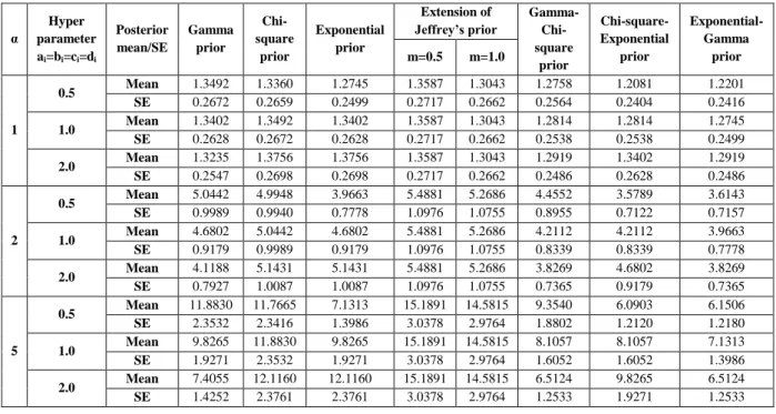
Table 1: Posterior Mean and SE for the posterior distribution using different priors with n=25.

α Hyper parameter ai=bi=ci=di Posterior mean/SE Gamma prior Chi-square prior Exponential prior Extension of Jeffrey’s prior Gamma- Chi-square prior Chi-square- Exponential prior Exponential-Gamma prior m=0.5 m=1.0 1 0.5 Mean 1.3492 1.3360 1.2745 1.3587 1.3043 1.2758 1.2081 1.2201 SE 0.2672 0.2659 0.2499 0.2717 0.2662 0.2564 0.2404 0.2416 1.0 Mean 1.3402 1.3492 1.3402 1.3587 1.3043 1.2814 1.2814 1.2745 SE 0.2628 0.2672 0.2628 0.2717 0.2662 0.2538 0.2538 0.2499 2.0 Mean 1.3235 1.3756 1.3756 1.3587 1.3043 1.2919 1.3402 1.2919 SE 0.2547 0.2698 0.2698 0.2717 0.2662 0.2486 0.2628 0.2486 2 0.5 Mean 5.0442 4.9948 3.9663 5.4881 5.2686 4.4552 3.5789 3.6143 SE 0.9989 0.9940 0.7778 1.0976 1.0755 0.8955 0.7122 0.7157 1.0 Mean 4.6802 5.0442 4.6802 5.4881 5.2686 4.2112 4.2112 3.9663 SE 0.9179 0.9989 0.9179 1.0976 1.0755 0.8339 0.8339 0.7778 2.0 Mean 4.1188 5.1431 5.1431 5.4881 5.2686 3.8269 4.6802 3.8269 SE 0.7927 1.0087 1.0087 1.0976 1.0755 0.7365 0.9179 0.7365 5 0.5 Mean 11.8830 11.7665 7.1313 15.1891 14.5815 9.3540 6.0903 6.1506 SE 2.3532 2.3416 1.3986 3.0378 2.9764 1.8802 1.2120 1.2180 1.0 Mean 9.8265 11.8830 9.8265 15.1891 14.5815 8.1057 8.1057 7.1313 SE 1.9271 2.3532 1.9271 3.0378 2.9764 1.6052 1.6052 1.3986 2.0 Mean 7.4055 12.1160 12.1160 15.1891 14.5815 6.5124 9.8265 6.5124 SE 1.4252 2.3761 2.3761 3.0378 2.9764 1.2533 1.9271 1.2533

(11)

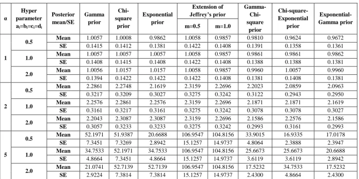
Table 2: Posterior Mean and SE for the posterior distribution using different priors with n=50. α Hyper parameter ai=bi=ci=di Posterior mean/SE Gamma prior Chi-square prior Exponential prior Extension of Jeffrey’s prior Gamma- Chi-square prior Chi-square- Exponential prior Exponential-Gamma prior m=0.5 m=1.0 1 0.5 Mean 1.0057 1.0008 0.9862 1.0058 0.9857 0.9810 0.9624 0.9672 SE 0.1415 0.1412 0.1381 0.1422 0.1408 0.1391 0.1358 0.1361 1.0 Mean 1.0057 1.0057 1.0057 1.0058 0.9857 0.9861 0.9861 0.9862 SE 0.1408 0.1415 0.1408 0.1422 0.1408 0.1388 0.1388 0.1381 2.0 Mean 1.0056 1.0157 1.0157 1.0058 0.9857 0.9960 1.0057 0.9960 SE 0.1394 0.1422 0.1422 0.1422 0.1408 0.1381 0.1408 0.1381 2 0.5 Mean 2.2861 2.2748 2.1619 2.3159 2.2696 2.2023 2.0859 2.0963 SE 0.3217 0.3209 0.3027 0.3275 0.3242 0.3122 0.2943 0.2950 1.0 Mean 2.2576 2.2861 2.2576 2.3159 2.2696 2.1871 2.1871 2.1619 SE 0.3161 0.3217 0.3161 0.3275 0.3242 0.3078 0.3078 0.3027 2.0 Mean 2.2043 2.3087 2.3087 2.3159 2.2696 2.1586 2.2576 2.1586 SE 0.3057 0.3233 0.3233 0.3275 0.3242 0.2993 0.3161 0.2993 5 0.5 Mean 52.1971 51.9387 20.6688 106.9547 104.8156 33.9015 16.9335 17.0178 SE 7.3451 7.3269 2.8942 15.1257 14.9737 4.8064 2.3888 2.3947 1.0 Mean 34.7533 52.1971 34.7533 106.9547 104.8156 25.6673 25.6673 20.6688 SE 4.8664 7.3451 4.8664 15.1257 14.9737 3.6119 3.6119 2.8942 2.0 Mean 21.0741 52.7139 52.7139 106.9547 104.8156 17.5232 34.7533 17.5232 SE 2.9224 7.3814 7.3814 15.1257 14.9737 2.4300 4.8664 2.4300

Table 3: Posterior Mean and SE for the posterior distribution using different priors with n=100.

α Hyper parameters ai=bi=ci=di Posterior mean/SE Gamma prior Chi-square prior Exponential prior Extension of Jeffrey’s prior Gamma- Chi-square prior Chi-square- Exponential prior Exponential-Gamma prior m=0.5 m=1.0 1 0.5 Mean 1.0436 1.0410 1.0327 1.0438 1.0334 1.0304 1.0198 1.0223 SE 0.1041 0.1040 0.1028 0.1044 0.1039 0.1032 0.1019 0.1020 1.0 Mean 1.0433 1.0436 1.0433 1.0438 1.0334 1.0328 1.0328 1.0327 SE 0.1038 0.1041 0.1038 0.1044 0.1039 0.1030 0.1030 0.1028 2.0 Mean 1.0429 1.0488 1.0488 1.0438 1.0334 1.0376 1.0433 1.0376 SE 0.1033 0.1044 0.1044 0.1044 0.1039 0.1027 0.1038 0.1027 2 0.5 Mean 2.7388 2.7320 2.6443 2.7628 2.7352 2.6818 2.5908 2.5972 SE 0.2732 0.2729 0.2631 0.2763 0.2749 0.2685 0.2588 0.2591 1.0 Mean 2.7154 2.7388 2.7154 2.7628 2.7352 2.6661 2.6661 2.6443 SE 0.2702 0.2732 0.2702 0.2763 0.2749 0.2660 0.2660 0.2631 2.0 Mean 2.6705 2.7524 2.7524 2.7628 2.7352 2.6360 2.7154 2.6360 SE 0.2644 0.2739 0.2739 0.2763 0.2749 0.2610 0.2702 0.2610 5 0.5 Mean 9.8139 9.7895 8.6027 10.2664 10.1637 9.2873 8.1900 8.2104 SE 0.9790 0.9777 0.8560 1.0266 1.0215 0.9299 0.8180 0.8190 1.0 Mean 9.4036 9.8140 9.4036 10.2664 10.1637 8.9409 8.9409 8.6027 SE 0.9357 0.9790 0.9357 1.0266 1.0215 0.8919 0.8919 0.8560 2.0 Mean 8.6879 9.8628 9.8628 10.2664 10.1637 8.3330 9.4036 8.3330 SE 0.8602 0.9814 0.9814 1.0266 1.0215 0.8251 0.9357 0.8251

The posterior mean, posterior standard error under all the assumed priors is calculated by assuming the different values of hyper parameters. From table 1 to 3, it is clear that the posterior standard error under the double prior Exponential-Gamma distribution are less as compared to other assumed priors, which shows that this prior is efficient as compared to other priors.

It is also observed that the posterior standard error under the double prior Exponential-Gamma distribution and Chi-square-Exponential distribution are almost same in all the sample sizes when the value of hyper parameter is

(12)

Conclusion

In this paper, the problem of Bayesian estimation for the generalized Rayleigh distribution, under different priors is considered. From the results, we observe that in most cases, Bayesian Estimator under the double prior Gamma - Exponential distribution has the less posterior standard error values. It is also observed that the standard error decreases as the sample size increases from 25 to 100.

References:

1. Ahmad, K.E., Fakhry, M.E. and Jaheen, Z.F. (1997). Empirical Bayes estimation of P(Y < X) and characterization of Burr-type X model, Journal of Statistical Planning and Inference, 64: 297-308.

2. Jaheen, Z.F. (1995). Bayesian approach to prediction with outliers from the Burr type X model, Microelectronic Reliability, 35: 45-47.

3. Jaheen. Z.F. (1996). Empirical Bayes estimation of the reliability and failure rate functions of the Burr type X failure model, Journal of Applied Statistical Sciences, 3: 281- 288.

4. Kundu, D and Raqab, M.Z., (2005). Generalized Rayleigh distribution different methods of estimations, Computational Statistics and Data Analysis, 49: 187- 200.

5. Mudholkar, G.S. and Srivastava, D.K. (1993). IEEE Transactions on Reliability, 42: 299 302.

6. Muhammad Aslam, (2008). Economic Reliability Acceptance Sampling Plan for Generalized Rayleigh Distribution, Journal of Statistics, 15: 26-35.

7. Raqab, M.Z. and Kundu, D. (2006). Burr type X distribution: revisited, Journal of Probability SS, 8: 179-198.

8. Reshi, J.A., Ahmed, A and Mir, K.A. (2013). Bayesian Estimation of Parameter of Size Biased Generalized Rayleigh Distribution Under The Extension of Jeffrey Prior And New Loss Functions, International Journal of Mathematical Research & Science, 1(3): 49-61.

9. Sartawi, H.A. and Abu-Salih, M.S. (1991). Bayes prediction bounds for the Burr type X model, Communications in Statistics - Theory and Methods, 20: 2307-2330.

10. Surles, J.G. and Padgett, W.J. (1998). Inference for P(Y < X) in the Burr type X model, Journal of Applied Statistical Science, 7: 225-238.

11. Surles, J.G., and Padgett, W.J. (2001). Inference for reliability and stress-strength for a scaled Burr type X distribution, Life time Data Analysis, 7: 187-200.

12. Surles, J.G., and Padgett, W.J. (2005). Some properties of a scaled Burr type X distribution, Journal of Statistical Planning and Inference, 72: 271-280.