Prediction of Sea Clutter Based on Recurrent Neural Network

(1)

Journal of Physics: Conference Series

PAPER • OPEN ACCESS

Prediction of Sea Clutter Based on Recurrent Neural Network

To cite this article: Wenyuan Wang et al 2021 J. Phys.: Conf. Ser. 1735 012008

View the article online for updates and enhancements.

(2)

Content from this work may be used under the terms of theCreative Commons Attribution 3.0 licence. Any further distribution

ICMSOA 2020

Journal of Physics: Conference Series 1735 (2021) 012008

IOP Publishing doi:10.1088/1742-6596/1735/1/012008

Prediction of Sea Clutter Based on Recurrent Neural Network

Wenyuan Wang1, Tingting Ji2 and Jinghao Sun1

1_{College of Information Science and Engineering, Ocean University of China, Qingdao,}

Shandong, China

2_{Teaching Center of Fundamental Courses, Ocean University of China, Qingdao, Shandong,}

China

E-mails: [email protected], [email protected]

Abstract. As radar sea clutter has chaotic characteristics, a prediction model can be established to predict sea clutter according to short-term predictability of chaotic time series. Therefore, this paper proposes a sea clutter amplitude prediction model based on LSTM, Stacked LSTM and Nested LSTM. This paper first obtains the best state space for sea clutter prediction according to the phase space reconstruction theory and establishes the prediction equation, then uses three networks to predict the sea clutter amplitude, and finally compares the effects of the three neural networks and analyzes the factors that affect the prediction precision. The experimental results on the IPIX radar data and P-band radar data show that, the model used in this paper has a smaller prediction error than RBF, and the prediction performance is better. The model can achieve high-precision and high-efficiency prediction of sea clutter and has verified the effectiveness of the method.

1.Introduction

Sea clutter is the backscattering echo from radar illuminating the sea surface. The analysis and research on the characteristics of sea clutter has not only theoretical significance, but also practical importance in applications such as sea surface target detection. For a long period of time, sea clutter is considered to be a completely random signal. Therefore, the research and processing of sea clutter mostly start from statistical theory. Researchers have proposed many statistical distribution models, such as Rayleigh distribution, log-normal distribution, Weibull distribution, compound K distribution. But these statistical models have limited application scope and cannot reflect the inherent sea clutter mechanism well.

In the 1990s, Simon Haykin and others repeatedly studied the sea clutter data, and confirmed chaotic characteristics of sea clutter. Meanwhile the chaotic time series has short-term predictability. Therefore, a prediction model can be established to study the internal nonlinear dynamics of sea clutter[1,2].

The research shows that the neural network can be used in the short-term prediction of sea clutter. In[3], Leung et al. used radial basis function (RBF) neural network to predict sea clutter, and used prediction error to detect sea ice. Subsequently, the team proposed to use multiple RBF neural networks to predict sea clutter, and experimental result showed that the effectiveness of this method is better than that of a single model[4]. Lu Ning et al. constructed a Generalized Regression Network (GRNN) target detector in[5], and completed target detection in sea clutter by using the difference in prediction errors between sea clutter and target echo. In 2015, Xu Ting proposed a sea clutter prediction method based on Genetic Wavelet Neural Network , which used IPIX radar data for multi-step prediction, and achieved better prediction effect than general neural network[6]. Zhao et al.proposed a method for predicting the near sea clutter power based on long short-term memory network, which achieved high prediction

(3)

ICMSOA 2020

2

accuracy[7]. Ma Liwen et al. predicted the amplitude of the measured sea clutter data using the gated cyclic network (GRU), and achieved good prediction results[8].

In this paper, three kinds of recurrent neural networks are used to predict the sea clutter amplitude, which are LSTM[9], stacked LSTM (stacked LSTM) and nested LSTM (nested LSTM) [10]. And then performance of the three networks in sea clutter prediction is analyzed. Finally the paper analyze the performance of the three networks in sea clutter prediction.

2.Nonlinear principle of sea clutter prediction

For chaotic time series, the establishment and prediction of chaotic model are carried out in phase space. Thus the reconstruction of phase space is a very important step for the processing of chaotic time series. 2.1.Phase space reconstruction

The basic idea of phase space reconstruction is: the evolution of any component in the system is determined by other components interacting with it. Therefore the information of these related components is implicit in the development of any component.

Takens proposed the embedding theorem in 1981. For an infinite one-dimensional scalar time series



x_i,1 i n



of d-dimensional chaotic attractor without noise, an m-dimensional embedded phase space can be found in the sense of topological invariance, as long as the dimension is

m



2 d

+

1

. According to Takens embedding theorem, a phase space in topological sense can be reconstructed from one-dimensional chaotic time series. There are two methods for phase space reconstruction: derivative reconstruction and coordinate delay reconstruction. The second method is used to reconstruct the phase space in this paper. For chaotic time series



x_i,1 i n



, the expression of phase space reconstruction is shown in equation (1):



, ,..., ( 1)



1, 2,...,

i i i i m

y = x x₊_ x₊ ₋ _ i= M (1)

Where y is the point in the phase space, τ is the delay time, m is the embedding dimension, and M is the number of points in the phase space, M = −n

(

m−1

)

. Therefore, the delay time τ and embedding dimension m need to be determined for the phase space reconstruction of chaotic time series.

2.1.1.Delay time τ. If the delay time τ is too small, the values of the two adjacent coordinate components in the phase space will be relatively close. Thus, two independent components cannot be obtained. Contrarily, the two adjacent coordinate components will be completely independent, and the projection of chaotic attractor trajectory in two directions will lose correlation. Therefore, it is necessary to choose a suitable τ to achieve a balance between independence and correlation. The commonly used methods to calculate the delay time include autocorrelation method, average displacement method, mutual information method and so on. In this paper, we use the mutual information method to calculate the delay time.

If the discrete time series is



x_i,1 i n



and P x_x

( )

_i is the probability density of point

 

x_i , then the information entropy of the sequence

 

x_i is:

( )

2

( )

1 log N x i x i i H X P x P x = = − (2)

Let

y

i

=

x

i+ , that is, the sequence

 

yi is a delay sequence of sequence

 

xi . Then the conditional

entropy of

 

y_i for

 

x_i is:

(

)

(

)

2

(

_{( )}

)

(

)

( )

, 1 , | N _xy _i, _i log xy i i = , i j _x _i P x y H Y X P x y H X Y H X P x = = −  − (3)

Where P_xy

(

x y_i, _i

)

is the joint probability density of the points

x

_i and

y

_i, and the joint entropy of the variables X and Y is defined as:

(4)

ICMSOA 2020

(

)

(

)

2

(

)

, , _xy _i, _i log _xy _i, _i i j H X Y = −P x y P x y (4)

From this, the mutual information of X and Y is:

(

,

)

( )

(

|

) ( )

=

( )

(

,

)

I Y X =H Y −H Y X H Y +H X −H X Y (5)

(

,

)

I Y X is a function related to delay time τ. In order to simplify calculation, τ corresponding to the minimum value of I Y X

(

,

)

is selected as the optimal delay time.

2.1.2.Minimum embedding dimension m. The embedding dimension is the minimum dimension to restore the chaotic dynamic system. If the m value is too small, the geometric structure of the chaotic system can not be completely expressed. If the m value is too large, the geometric structure of the original system can be completely expressed in theory. But at the same time, the calculation amount will be increased and the noise will be amplified. For the determination of the minimum embedding dimension, the commonly used methods include geometric invariant , false nearest neighbors and Cao method. In this paper, Cao method is used. In this method, only the delay time τ is needed and the embedding dimension m can be obtained with a small amount of data.

For time series



x_i,1 i n



, when the delay time is τ and the embedding dimension is m, the Y mi

( )

is Y m_i

( )

=



x x_i, _i+_, ,x_i+₍_m−₁₎_



and its nearest neighbor YiNN

( )

m is

( )



, , , ( 1)



NN NN NN NN

i i i i m

Y m = x x₊_ x₊ ₋ _ .

Three variables are be defined with:

( )

(

)

(

)

( )

2 1 1 , NN i i NN i i Y m Y m a i m Y m Y m + − + = − (6)

( )

2

( )

1 1 , N m i E m a i m N m   − = =  − (7)

( )

₍

( )

₎

1 1 E m E m E m = + (8)

For a certain time series, E m1

( )

will not change after m is greater than a certain fixed value m0, and the value of m0 can be used as the best embedding dimension of phase space reconstruction. However, for random sequences, with the increase of m, E m1

( )

not reaching a stable value, so it is difficult to

distinguish whether E m₁

( )

is slowly changing or converging. Thus a definition is added:

( )

* 1 1 N m NN i m i m i E m x x N m     − + + = =  − − (9)

( )

(

)

( )

* 2 _* 1 E m E m E m + = (10)

If there is no correlation between the data, E2

( )

m is always equal to 1. For chaotic time series, the

correlation between data depends on the value of m. Thus there always exists m so that E₂

( )

m is not equal to 1. According to the curves of E m₁

( )

and E₂

( )

m , we can find the minimum embedding dimension m when E m₁

( )

tends to be stable and E₂

( )

m is not equal to 1.

2.1.3.Sea clutter prediction equation. If the sea clutter sequence is



x_i,1 i n



, the expression of the sea clutter phase space reconstruction is as follows:



,

( 1)



i m i i i m

(5)

ICMSOA 2020

4

The above equation is the sea clutter prediction equation. If the expression of the state equation F can be obtained, the sea clutter prediction can be carried out through this equation. In order to increase the amount of information in the system and enhance the prediction equation in function generalization, this paper actually uses the prediction equation proposed by S.Haykin in [11]:



,

1

,

2

,

1



i m i i i i m

x

₊ _

=

F x x

₊

x

₊

x

₊ _₋ (12)

3.Network model principle

Recurrent neural network (RNN) is a kind of neural network with short-term memory capability, which is suitable for dealing with time-related problems.Long short-term memory network (LSTM) is a kind of RNN, which can solve the problem of long-distance dependence and gradient disappearance of RNN. LSTM and its variants are used to solve various problems, especially in text generation, speech recognition, handwriting recognition and so on.

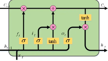
Compared with one state normal RNN, there are four states in LSTM. The LSTM’s loop structure keeps a persistent unit state, which is used to decide whether the information should be forgotten or passed on. The internal diagram of LSTM’s loop structure is shown in Figure 1. Each loop structure has two outputs, where C_tis the unit state and h_t is the output of the network.

Figure 1. The LSTM architecture.

LSTM cells are composed of input gate, forget gate, output gate and cell state. The state update formula of each gate is as follows:

Input gate:

(

1

)

t t xi t hi i i = x W +h W₋ +b (13) Forget gate:

(

1

)

t t xf t hf f f = x W +h W− +b (14) Cell state:

(

)

1 1 t t t t t xc t hc c c = f c₋ +i  x W +h W₋ +b (15) Output gate:

(

1

)

t t xo t ho o o = x W +h W₋ +b (16) Final output:

( )

t t t h =o  c (17)

Where i_t, f_t and o_t are the outputs of input gate, forget gate and output gate respectively; c_tand h_tare cell state and output respectively; W and B are weight matrix and bias matrix respectively.

Stacked LSTM uses multiple layers LSTM for stacking, in which the output of the upper layer is used as the input of the next layer.

(6)

ICMSOA 2020

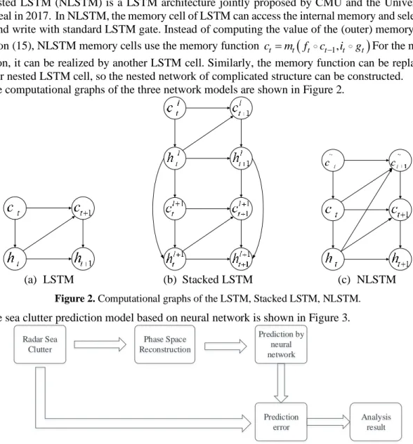
Nested LSTM (NLSTM) is a LSTM architecture jointly proposed by CMU and the University of Montreal in 2017. In NLSTM, the memory cell of LSTM can access the internal memory and selectively read and write with standard LSTM gate. Instead of computing the value of the (outer) memory cell as equation (15), NLSTM memory cells use the memory function c_t =m_t

(

f_t c_t₋₁,i_t g_t

)

For the memory function, it can be realized by another LSTM cell. Similarly, the memory function can be replaced by another nested LSTM cell, so the nested network of complicated structure can be constructed.

The computational graphs of the three network models are shown in Figure 2.

(a) LSTM (b) Stacked LSTM (c) NLSTM

Figure 2. Computational graphs of the LSTM, Stacked LSTM, NLSTM. The sea clutter prediction model based on neural network is shown in Figure 3.

Radar Sea Clutter Phase Space Reconstruction Prediction by neural network Prediction error Analysis result

Figure 3. Flow chart of sea clutter prediction.

4.

Experiment and result analysis

4.1.Data introduction

The data used in this paper includes two parts: The first part of the data comes from IPIX radar data from McMaster University Laboratory in Canada in 1993. This experiment uses four sets of data #26, #54, #320, and #310 corresponding to 1-4 levels of sea state. Each group of data contains 14 range gates, including one main target gate, two or three secondary target gates, and the rest are sea clutter gates. Each range gate has 131,072 sampling points. The second part of the data is the sea clutter data collected by the P-band radar on the Yellow Coast of China. This experiment uses four sets of P-band data, which are P101, P201, P301, and P401 corresponding to 1-4 levels of sae state. Each group of data contains 100 range gates, all of which are sea clutter gates. Each range gate has 61,001 sampling points.In this experiment, the amplitude of sea clutter is predicted. So it is necessary to model and normalize the original data. The amplitude of sea clutter data of the fourth range gate in #26 and the first range gate in P101 are shown in Figure 4.

(7)

ICMSOA 2020

6

(a) IPIX radar sea clutter data (b) P-band radar sea clutter data Figure 4. Normalized amplitude figure of IPIX radar and P-band radar

4.2.Experiments

The experiment uses the mutual information method and the Cao method to obtain the delay time τ and embedding dimension m of each group of data, constructs the sea clutter prediction equation according to formula (12), and then uses the four network models of LSTM, Stacked LSTM, NLSTM and RBF to predict sea clutter and compare the prediction effects of the four networks. The experimental training set is 5000 sampling points, the validation set is 1500 sampling points, and the test set is 1500 sampling points. Choose the root mean square error function (RMSE) as the evaluation function to evaluate the prediction results:

(

)

2 1 1 n i i i

RMSE predicted real

n =

=  − (18)

The first part of the experiment is to predict the sea clutter data of different range gates in the same file. The radar pulses used in different range gates are the same, and the sea conditions such as radar azimuth, wind speed and wind direction are similar. The experiment uses the #26 data of the IPIX radar data. The seventh gate of the data is the main target gate, the sixth and eighth gates are secondary target gates, and the rest are sea clutter gates.The prediction results of the network are shown in Table 1, where the data is the RMSE value predicted by the network, and n is the number of hidden layers of the network . From Table 1, we can see that the network has relatively low prediction errors for the sea clutter data of the same file at different ranges, and this can meet the accuracy requirement of sea clutter prediction.The experimental results show that the network model has good prediction effect for all data of the same file.

The second part of the experiment predicts the sea clutter data corresponding to the four sea states. We use the #26, #54, #320 and #310 data of the IPIX radar data corresponding to 1-4 levels of sea state and the P101, P201, P301 and P401 data of the P-band radar data corresponding to 1-4 levels of sea state respectively. The experimental results are shown in Table 2.

From the experimental results in Table 2, it can be seen that when the sea state is high, the prediction error of IPIX radar sea clutter increases significantly, and the prediction performance of both the RBF and the three networks proposed in this paper has decreased. This is because in high sea state, the sea surface fluctuates violently and the internal mechanism of sea clutter is more complicated due to the influence of wind speed and other conditions, which leads to decline of the prediction effect of the network.The RMSE of the P-band radar sea clutter is lower than that of the IPIX radar sea clutter, and the prediction is more accurate. This is because the amplitude of the P-band sea clutter changes slowly.

(8)

ICMSOA 2020

Table 1. Prediction error of each sea clutter gate in #26 Model RBF LSTM Stacked LSTM NLSTM Stacked LSTM NSLTM n 1 1 2 2 3 3 1 0.0307 0.0276 0.0248 0.0248 0.0265 0.0265 2 0.0185 0.0157 0.0156 0.0157 0.0163 0.0156 3 0.0318 0.0244 0.0246 0.0236 0.0262 0.0241 4 0.0257 0.0285 0.0255 0.0237 0.0276 0.0247 5 0.0269 0.0288 0.0236 0.0227 0.0235 0.0230 9 0.0545 0.0315 0.0309 0.0290 0.0344 0.0326 10 0.0191 0.0194 0.0180 0.0175 0.0182 0.0180 11 0.0396 0.0270 0.0272 0.0263 0.0279 0.0281 12 0.0322 0.0184 0.0204 0.0190 0.0211 0.0198 13 0.0315 0.0229 0.0238 0.0225 0.0248 0.0247 14 0.0150 0.0115 0.0118 0.0118 0.0115 0.0120

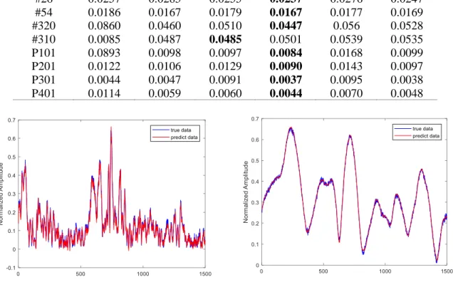
Table 2. Sea clutter prediction results of four sea state Model RBF LSTM Stacked LSTM NLSTM Stacked LSTM NSLTM n 1 1 2 2 3 3 #26 0.0257 0.0285 0.0255 0.0237 0.0276 0.0247 #54 0.0186 0.0167 0.0179 0.0167 0.0177 0.0169 #320 0.0860 0.0460 0.0510 0.0447 0.056 0.0528 #310 0.0085 0.0487 0.0485 0.0501 0.0539 0.0535 P101 0.0893 0.0098 0.0097 0.0084 0.0168 0.0099 P201 0.0122 0.0106 0.0129 0.0090 0.0143 0.0097 P301 0.0044 0.0047 0.0091 0.0037 0.0095 0.0038 P401 0.0114 0.0059 0.0060 0.0044 0.0070 0.0048

(a) Prediction results of #26 (b) Prediction results of P101 Figure 5. Prediction results of partial sea clutter data of IPIX radar and P-band radar 4.3.Prediction performance analysis of network

Based on the results of the above experiments, we compare and analyze the prediction performance of the network, and look into the factors that affect the prediction accuracy of the network.

1. Comparison of prediction results of LSTM, Stacked LSTM, NLSTM and RBF: Overall, the predicted RMSE of the three networks used in this paper are lower than those predicted by RBF, and

(9)

ICMSOA 2020

8

the prediction result is better than RBF. Especially in the prediction of sea clutter data with high sea states, the prediction performance of the three network is much better than that of the RBF. The experimental results show that the prediction performance of RNN (LSTM, Stacked LSTM, NLSTM) model is better than RBF in the prediction of sea clutter.

2. Comparison of the prediction effects of the three network models of LSTM, Stacked LSTM, and NLSTM:

1). For different hidden layers: From the prediction performance of one-layer LSTM, two-layer Stacked LSTM and three-layer Stacked LSTM model, the prediction performance of the network gradually decreases as the number of layers increases. Generally, the performance of one-layer LSTM is the most well, and the three-layer Stacked LSTM is the worst. For the NLSTM network, the predicted RMSE value of the two-layer NLSTM network is lower than the predicted RMSE value of the three-layer NLSTM. This result shows that for the prediction of sea clutter data, the increase in the number of network layers cannot bring about the improvement of the regression prediction effect for the prediction of sea clutter data. The increase in the number of layers will not only bring about exponential growth of time and memory costs, but also easily cause gradients to disappear. In addition, the model is a time series model, resulting in slowed update iterations of the LSTM layer close to the input layer and reduced convergence effects.

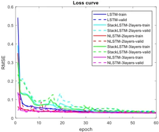
2). For the same hidden layer, the prediction effect comparison of Stacked LSTM and NLSTM: From the experimental results in Table 1 and Table 2, whether it is a two-layer NLSTM or a three-layer NLSTM, the predicted RMSE of the network is lower than the RMSE predicted by stacked LSTM with the same number of hidden layers. NLSTM increases depth by nesting instead of stacking, and can achieve a more efficient temporal hierarchy than traditional Stacked LSTM. Therefore, compared with Stacked LSTM with the same number of parameters, the prediction performance of NLSTM is better. Figure 6 shows the changes of RMSE values during training and verification of the three networks on the data of the fourth range gate in #26. It can be seen from Figure 6, all the RMSE values of the networks are decreae, and basically reach a relatively stable level after 50 times as the number of iterations increases. The RMSE convergence speed of the two Stacked LSTM networks is slower than the convergence speed of the others and the final RMSE value is larger, The RMSE of the two NLSTM networks converges fastest, and can converge to a lower value after less iterations. This also corresponds to Table 1 and Table 2. NLSTM has the lowest overall RMSE value and the best prediction performance on all test data sets.

Figure 6. Loss curve in the process of network training and verification

5.Conclusion

In this paper, we use phase space reconstruction to study sea clutter from the perspective of chaos and propose to use LSTM, Stacked LSTM and NLSTM to predict the amplitude of sea clutter. The experiment analyzes the prediction performance of the three networks from many aspects. And the

(10)

ICMSOA 2020

results show that the three networks used in this paper have higher prediction accuracy of sea clutter amplitude than traditional RBF. Since NLSTM is more suitable for processing long-term sequences in structure, the prediction effect is better than that of the other two.

The experimental results in this paper can also serve as reference for practical applications such as sea surface target detection. In the future, the network model will be improved in view of the problems existing in the network model, such as long training time, large prediction error and poor effect in high sea clutter prediction.

Acknowledgments

This work was supported by Equipment Pre-research Key Laboratory Fund Project(6142403190304).

References

[1] Haykin S and Puthusserypady S 1997 Chaotic dynamics of sea clutter Chaos An Interdiplinay Journal of Nonlinear ence 7(4): 777-802.

[2] Haykin S and Puthusserypady S 1997 Chaos, sea clutter, and neural networks Proc. of The 31st Asilomar Conf. on Signals, Systems amd Computers p 1224-1227.

[3] Leung H and Lo P 1993 Chaotic radar signal processing over the sea IEEE Journal of Oceanic Engineering 18(3): 287-295.

[4] Xie N, Leung H, Chan H 2003 A multiple-model prediction approach for sea clutter modeling IEEE Trans. on Geoscience and Remote Sensing 41(6): 1491-1502.

[5] Ning Lu, Cai Yu and Wei Cai 2012 GRNN small target detection based on sea clutter Fire Control Radar Technology 41(2): 4-7.

[6] Ting Xu 2015 Prediction of sea clutter based on GA-WNN Electronic Design Engineering 23(18): 34-37.

[7] Jun Zhao, Jiaji Wu, Xiaowei Guo, Jie Han, Kai Yang, Hongguang Wang 2019 Prediction of radar sea clutter based on LSTM Journal of Ambient Intelligence and Humanized Computing

DOI: 10.1007/s12652-019-01438-4

[8] Liwen Ma, Jinpeng Zhang, Jiaji Wu, Yushi Zhang, Peng Zhao and Xiaoyuan Xia 2020 Prediction of sea clutter using gated feedback recurrent neural network Chinese Journal of Radio Science 35(2): 257-263.

[9] Cers F A, Schmidhuber J, Cummins F 2000 Learning to Forget: Continual Prediction with LSTM Neural Computation 12(10): 2451-2471.

[10] Moniz J R A and Krueger D 2017 Nested LSTMs Proc. of Asian Conf. on Machine Learning (80): 1-15.