Scholar Commons
Mathematics and Statistics Faculty Publications
Mathematics and Statistics
2016
The Statistics and Mathematics of High Dimension
Low Sample Size Asymptotics
Dan Shen
University of South Florida, [email protected]
Haipeng Shen
University of Hong KongHongtu Zhu
University of North Carolina
J S Marron
University of North Carolina
Follow this and additional works at:
http://scholarcommons.usf.edu/mth_facpub
Part of the
Physical Sciences and Mathematics Commons
This Article is brought to you for free and open access by the Mathematics and Statistics at Scholar Commons. It has been accepted for inclusion in Mathematics and Statistics Faculty Publications by an authorized administrator of Scholar Commons. For more information, please contact
Scholar Commons Citation
Shen, Dan; Shen, Haipeng; Zhu, Hongtu; and Marron, J S, "The Statistics and Mathematics of High Dimension Low Sample Size Asymptotics" (2016).Mathematics and Statistics Faculty Publications. 5.
THE STATISTICS AND MATHEMATICS OF HIGH DIMENSION LOW SAMPLE SIZE ASYMPTOTICS
Dan Shen1, Haipeng Shen2, Hongtu Zhu3 and J. S. Marron3 1University of South Florida, 2University of Hong Kong
and 3University of North Carolina at Chapel Hill
Abstract: The aim of this paper is to establish several theoretical properties of principal component analysis for multiple-component spike covariance models. Our results reveal an asymptotic conical structure in critical sample eigendirections un-der the spike models with distinguishable (or indistinguishable) eigenvalues, when the sample size and/or the number of variables (or dimension) tend to infinity. The consistency of the sample eigenvectors relative to their population counterparts is determined by the ratio between the dimension and the product of the sample size with the spike size. When this ratio converges to a nonzero constant, the sample eigenvector converges to a cone, with a certain angle to its corresponding population eigenvector. In the High Dimension, Low Sample Size case, the angle between the sample eigenvector and its population counterpart converges to a limiting distri-bution. Several generalizations of the multi-spike covariance models are explored, and additional theoretical results are presented.
Key words and phrases: Big data, conical behavior, high dimension low sample size, PCA.
1. Introduction
As the field of statistics continues to evolve, there is ongoing discussion about the role that should be played by mathematics. There are those who wish to focus on data as much as possible, and thus base their work on experiential insights, and those who never actuaIly work with data, but instead develop mathematical ideas about how data should be analyzed. Among the many mathematical methods that have been used to gain statistical insights, asymptotic techniques stand out as having provided a large number of insights over the years.
What is the value of asymptotics? Some might say one should not consider asymptotics on the grounds that one never has an infinite sample size, while others view asymptotics as “understanding what happens in situations where the sample size grows”. Some take the latter notion to an extreme by insisting that all asymptotics should “follow some type of sampling process”. We bring in a different view of asymptotics, in which the focus is moved beyond mere sampling to any type of limiting operation that gives statistical insights. It will
be seen that the role of asymptotic insights can go beyond academic indulgence to understanding even the most basic statistical concepts in challenging modern data analytic settings.
A currently fashionable statistical topic is Big Data. This notion goes well beyond a large sample size and includes high dimension, but, while the size of modern data sets indeed presents serious statistical challenges, complexity
of modern data sets is an even more serious and challenging aspect. Useful terminology for approaching a complex data set is object oriented data analysis, introduced in Wang and Marron (2007) and more recently discussed in Marron and Alonso (2014).
There has been a realization by many that asymptotics should include cal-culation of limits as the dimension grows. For example, in the biological field of gene expression, the technology of microarrays (see Murillo et al. (2008) for an overview) enabled the measurement of expressions of tens of thousands of genes at once, and one could say this leads to vectors effectively understood by a limiting process of growing dimension. Others might contend that such a limit is inappropriate. This line of discussion could be continued in the direction of RNAseq techonology (see Denoeud et al. (2008) for an introduction), where instead of a single number for each gene, expression estimates at the level of resolution of genetic base pairs are available, thus resulting in a factor of around ten thousand more dimensions. Here we argue thatthe goal of asymptotics is to find insightful simple structures that underly complex statistical contexts.
There are a number of ways that growing dimension asymptotics have been studied. Pioneering work by Portnoy (1984) and Portnoy et al. (1988) studied cases where the dimension grew relatively slowly, resulting in an asymptotic do-main that was not far from classical fixed-dimensional analysis. Another asymp-totic domain, random matrix theory, arises when the dimension and sample size grow at the same rate. Work in this area has been done mostly outside the sta-tistical community, with landmark results including Marcenko and Pastur (1967) on the distribution of eigenvalues of the sample covariance matrix, and Tracy and Widom (1996) on the distribution of the largest eigenvalue. A good overview of the literature in this area can be found in Bai and Silverstein (2009). Statis-tical implications have been developed in a series of papers by Johnstone and co-authors, see e.g., Johnstone and Lu (2009), and a number of others since.
An asymptotic domain whose importance has only recently begun to be recognized has the dimension growing more rapidly than the sample size. Hall, Marron, and Neeman (2005) coined the terminologyhigh dimension, low sample size (HDLSS) for the case where the sample size is fixed while the dimension grows.
2. HDLSS Backround
As noted in Hall, Marron, and Neeman (2005), the world of HDLSS asymp-totics is full of concepts and ideas that can run counter to intuition, many of which are discussed in the following. For example, in the limit as the dimension
d→ ∞ with a fixed sample size n, a standard Gaussian sample will lie near the surface of a growing sphere of radius d1/2 and the angle between each pair of points with vertex at the origin will approach 90◦. Thus the increasing random-ness inherent in growing dimension tends towards random rotation and, modulo that random rotation and scaling by a factor ofd−1/2, the data tend to lie near vertices of the unit simplex. This phenomenon, geometric representation, leads to a number of interesting statistical insights.
Beran (1996) and Beran et al. (2010) have it that some of these ideas lie at the heart of the famous paper of Stein (1956) on inadmissability of the sample mean. Early use of HDLSS asymptotics in the Stein estimation context can be found in Casella and Hwang (1982).
A closely related asymptotic domain is the ultra high dimension of Fan and Lv (2008), who consider the case of d=exp(cna), for constants c and a, in the classical limit asn→ ∞. The ultra high case can also be equivalently formulated as n= (log(d)/c)1/a in the limit as d→ ∞. The later formulation reveals that this case is quite near to the HDLSS context.
The HDLSS geometric representation has been established under a range of conditions. Hall, Marron, and Neeman (2005) went beyond the independent Gaussian case by assuming the data vectors satisfy a mixing condition. Ahn et al. (2007) proposed a more palatable eigenvalue condition for geometric represen-tation. In unpublished correspondence John Kent pointed out, using a Gaussian scale mixture example, that more than univariate moment conditions are needed. Conditions that are especially appealing, because they are based only on the co-variance matrix (with no assumption of Gaussianity), have been developed in a series of papers Yata and Aoshima (2009, 2010b); Aoshima and Yata (2011); Yata and Aoshima (2012a); Aoshima and Yata (2015). A non-Gaussian condi-tion that makes intuitive sense based on the types of data found in genomics can be found in Jung and Marron (2009).
3. PCA and HDLSS Asymptotics
PCA is a well-proven workhorse method for many tasks involving high-dimensional data, see Jolliffe (2005) for excellent introduction and overview. A strong indicator of its utility comes from the fact that it has been rediscovered and renamed a number of times. For example, it is called empirical orthogonal
functions in the earth / climate sciences,proper orthogonal decomposition in ap-plied mathematics, theKarhunen Loeve expansion in electrical engineering and probability, and factor analysis in a number of non-statistical areas.
One can motivate PCA from a Gaussian likelihood viewpoint, but it is more generally viewed as a fully nonparameteric method, with a number of uses. While PCA is a common dimension reduction method, it is arguably even more useful for data visualization in high-dimensional contexts, for example in Functional Data Analysis, see Ramsay and Silverman (2002), Ramsay (2005), and Ferraty and Vieu (2004).
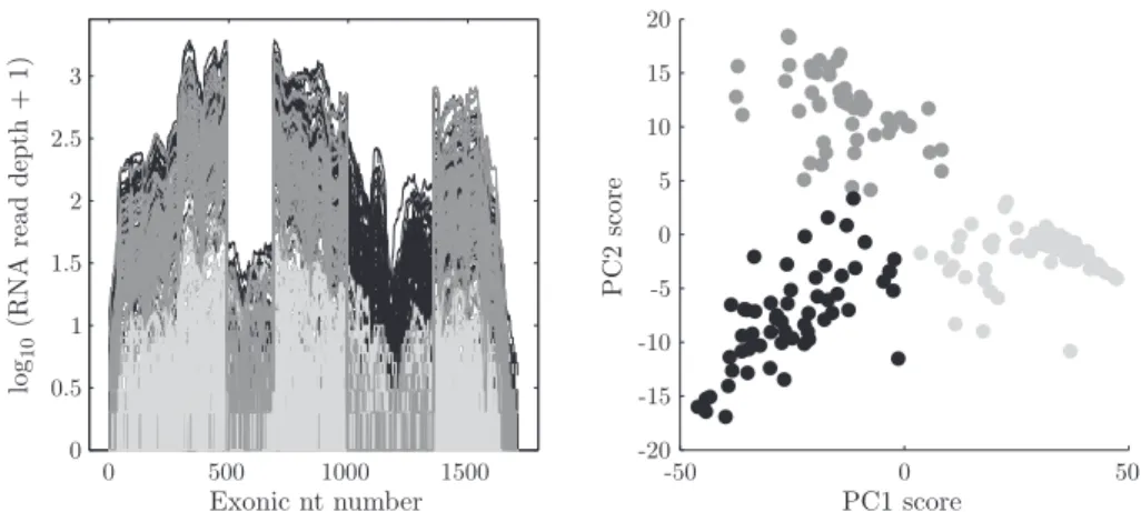
An example of PCA data visualization is shown in Figure 1. The curves in the left panel are read depth curves from RNAseq measurements Wilhelm and Landry (2009) of n = 180 lung cancer patients. Each curve is a detailed measurement of biological expression of the gene CDKN2A for one tissue sample, with the horizontal axis indicating d= 1,709 base pair locations of the reference genome, and the height of the curve a log10 count that indicates level of gene expression. Insight into how the curves relate to each other comes from the PCA scatterplot in the right panel of Figure 1. The axes of the scatterplot are the first two principal component scores. There is some apparent interesting structure, in the form of three distinct clusters. To explore the relevance of these clusters, they have been brushed, i.e., colored with grey levels. These same colors have been used on the curves in the left panel. The lightest grey curves tend to be much lower than the others, representing cases where the CDKN2A gene is essentially not expressed (typical in some cases). The genome location of the gene includes several disconnected loci called exons, which here have been connected giving the block-like structure apparent in the other curves. The third exon shows very low levels of expression for all cases. The fifth exon is interesting because it is fully expressed for only the black cases, while all others show a very low level of expression. This phenomenon is calledalternate splicing, and is very important in cancer research because it can become the target of drug treatments. This example motivated a search for alternate splice events, based on screening for clusters in read depth curves, over all genes. An important challenge to the implemention of this was the assessment of the statistical significance of clusters in very high dimensions, done using the SigClust method of Liu et al. (2008). This screening method was named SigFuge by Kimes and Cabanski (2013), who reported on the results of a full genome screen that found previously unknown splicing events, one of which was then confirmed by a biological experiment. The point is that PCA found important structure in this HDLSS data set through visualizing the PC scores.
The asymptotic underpinnings of PCA in HDLSS contexts were first consid-ered by Ahn et al. (2007), and more deeply by Jung and Marron (2009). Insight
Figure 1. PCA of RNAseq log read depth maps, for the union of exons in the gene CDKN2A. Left panel shows data curves. Right panel is the PC1 vs. Pc2 scores scatterplot, showing three distinct clusters (brushed with gray levels). Use of these same colors in the left panel shows essentially unexpressed cases (lightest grey), and a clear alternate splicing event (other grey shades). This is an HDLSS example where PCA clearly reveals important biological structure.
into the behavior of PCA comes from study of the spike covariance model, made popular in statistics by Paul (2007) and Johnstone and Lu (2009). In the simplest form of the spike covariance model, there is a single large eigenvalue with the rest much smaller and constant, where the largest eigenvalue has size of growing order dα. The key result is that, in the limit asd→ ∞ withn fixed, letting u1
and ˆu1 denote the first population and sample eigenvectors respectively,
angle<uˆ1, u1 >→
{
90◦for α <1,
0 for α >1. (3.1)
This defines a notion ofconsistency when the spike is large,α >1, and a notion ofstrong inconsistency when the spike is small,α <1. One or the other holds in almost all such settings, with the exception ofα= 1. The boundary atα= 1 can be understood from the geometric representation: in the HDLSS limit, standard Gaussian data tends to lie on the surface of the sphere at the origin, with radius
d1/2. In the spike model, whenα >1, the distribution reaches outside this sphere (eigenvalues are on the scale of variance, so the largest standard deviation is much greater thand1/2), which results in consistency of the first eigendirection. When
α < 1, the distribution is essentially contained within the sphere, so the first eigendirection is random, and random directions are asymptotically orthogonal to any given direction.
Related results are available in Yata and Aoshima (2009, 2010a, 2012a, 2013). New insights about sparse PCA were dicovered by Shen, Shen, and Marron
(2012a); See Shen, Shen, and Marron (2012b) for broader results in this spirit, including all combinations ofnanddtending to infinity. Limiting behavior when
α = 1 was first explored by Jung, Sen, and Marron (2012) in the HDLSS case. Yata and Aoshima (2012a) proposed a noise reduction estimator that relaxes the boundary of the eigenvalue estimator toα = 1/2 in the HDLSS case.
While under a sufficiently strong signal in the covariance structure, PCA can find the right direction vectors, estimation of the eigenvalues is more challeng-ing. Indeed, letting λ1 and ˆλ1 denote the population (and sample resp.) first
eignevalues, there are a number of results in the spirit of ˆ λ1 λ1 L −→ χ2n n , (3.2)
under various HDLSS conditions. Thus sample eigenvalues are generally incon-sistent when the sample size is fixed but, as noted by Yata and Aoshima (2009, 2010b), sample eigenvalues are consistent if it is assumed that, in addition to
d→ ∞,n→ ∞as well. Where n grows more slowly thand, one speaks of High Dimension Moderate Sample Size, Borysov, Hannig, and Marron (2014). Yata and Aoshima (2010a, 2012a, 2013) have given modified versions of PCA that provide consistent eigenvalue estimates.
4. Understanding Variation in Scores
In HDLSS situations PCA scores, which form the basis of informative scat-terplots, such as Figure 1, are generally inconsistent in the HDLSS limit. In particular, the ratio of the sample and population PC scores converge to a non-degenerate random variable, as formulated here.
In Section 4.2, we show that, for a given component, the ratios for each data point indeed converge to a random variable, but it is the same realization of the random variable for each data point. Thus, while all the scores are off by a random factor, it is the same factor for each data point; in scatterplots the axis labels are off by a random factor, but the relationship between points is still correct.
This issue was presaged in Yata and Aoshima (2009) and is quite similar to the eignevalue inconsistency at (3.2). The improved variation of PCA proposed in Yata and Aoshima (2012a, 2013) gives asymptotically correct scalings. Under the random matrix framework, Lee, Zou, and Wright (2010) showed that the ratios of the sample and population PC scores converge to a constant. Hellton and Thoresen (2014) have used the ideas of pervasive signal and visual content
4.1. Assumptions and notation
If{(λk, uk) :k= 1,· · ·, d}are the eigenvalue-eigenvector pairs of the
covari-ance matrix Σ such thatλ1≥λ2 ≥. . .≥λd>0, we can write
Σ =UΛUT, (4.1) where Λ = diag(λ1, . . . , λd) andU = [u1, . . . , ud].
Assumption 1. X1, . . . , Xn are i.i.d. d-dimensional random sample vectors with the representation
Xi = d
∑
j=1
λ1j/2zi,juj, (4.2) where the zi,j’s are i.i.d. random variables with zero mean, unit variance, and finite fourth moment.
An important special case has the Xis’ N(0,Σ). Consider that the Xi are
i.i.d.N(ξ,Σ) withξ ̸= 0. As in Paul and Johnstone (2007), it is well known that
n
∑
i=1
(Xi−X)(Xi−X)T has the same distribution as n−1
∑
i=1
YiYiT,
where X is the sample mean and Yi are i.i.d. N(0,Σ). Then the asymptotic
properties of PCA can be studied throughYi. Since the sample covariance matrix
is location invariant, we can assume without loss of generality that Xi has zero
mean at least for the normal case. In general, one has to consider the theoretical properties ofX−µ; these have been widely investigated in the literature Rollin (2013); Chernozhukov, Chetverikov, and Kato (2014) even whendis much larger thann.
Denote the jth normalized population PC score vector by
Sj = (S1,j, . . . , Sn,j)T =λ−j1/2(uTjX1, . . . , uTjXn)T, j= 1, . . . , d. (4.3)
Denote the data matrix byX = [X1, . . . , Xn] and the sample covariance matrix
by ˆΣ = (1/n)XXT. The sample covariance matrix can be decomposed as ˆ
Σ = ˆUΛ ˆˆUT, (4.4) where, similarly, ˆΛ = diag(ˆλ1, . . . ,λˆd) and ˆU = [ˆu1, . . . ,uˆd]. Since
n−1/2X= d ∑ j=1 ˆ λ1j/2uˆjvˆjT, where ˆvj = (ˆv1,j, . . . ,vˆn,j)T, j= 1,· · ·, d,
thejth normalized sample PC score vector is ˆ
Sj = ( ˆS1,j, . . . ,Sˆn,j)T =n1/2(ˆv1,j, . . . ,ˆvn,j)T, j = 1, . . . , d. (4.5)
Let {ak : k = 1, . . . ,∞} and {bk : k = 1, . . . ,∞} be two sequence of
con-stants, wherekcan stand for eithernord. We writeak≫bkif limk→∞bk/ak= 0,
andak∼bk ifc2≤limk→∞ak/bk≤limk→∞ak/bk≤c1for constantsc1 ≥c2 >0.
If{ξk:k= 1, . . . ,∞}is a sequence of random variables and {ek:k= 1, . . . ,∞}
is a sequence of constants, we write ξk = Oa.s(ek) if limk→∞|ξk/ek| ≤ζ almost
surely withP(0< ζ <∞) = 1.
4.2. HDLSS inconsistency
In this subsection, we show the asymptotic properties of PC scores in HDLSS when the sample sizenis fixed and the dimensiond→ ∞. We consider multiple spike models Jung and Marron (2009) under which, as d→ ∞,
λ1≫ · · · ≫λm ≫λm+1∼ · · · ∼λd∼1, (4.6)
wherem∈[1, n∧d] is finite. Under these spike models, Jung and Marron (2009) showed that whenn is fixed, ifd/λm →0, the angle between each of the firstm
sample eigenvectors ˆuj and its corresponding population eigenvector uj goes to
0 with probability 1, the consistency of the sample eigenvector.
However, under the same assumptions, the sample PC scores are not consis-tent. We show that, for a particular principal component, the proportion between the sample PC scores and the corresponding population scores converges to a random variable, the realization of which remains the same for all data points. Since we study ˆSi,j/Si,j, we need to assume
P(zi,j ̸= 0) = 1, i= 1, . . . , n, j= 1, . . . , m, (4.7)
to ensure thatP(Si,j ̸= 0) = 1 (Si,j =zi,j from (4.2) and (4.3)). Let
e
Zj = (z1,j, . . . , zn,j)T and Rj =
e
ZjTZej
n , j= 1, . . . , d, (4.8)
wherezi,j is defined in (4.2).
Theorem 1. Under Assumption 1, (4.6), and (4.7), for fixed n as d → ∞, if
d/λm →0, then ˆ Si,j Si,j a.s −−→R−j1/2, i= 1, . . . n, j = 1, . . . , m, (4.9)
where−−→a.s stands for almost sure convergence. In addition, if Assumption1holds with normal zi,j’s, then nRj is the Chi-square with n degrees of freedom.
Remark 1. The results in Theorems 1 differ from those in Lee, Zou, and Wright (2010). Under the random matrix framework with n ∼ d → ∞ and λj < ∞,
Lee, Zou, and Wright (2010) showed that the ratios between the sample and population eigenvalues converge to a constant. Lee, Zou, and Wright (2010) did not consider properties of PC scores under the framework of our Theorem 2.
Remark 2. As the ratio Rj only depends on j, scores scatter plots, such as
right panel of Figure 1, have incorrectly labeled axes but asymptotically correct relative positions of points.
Remark 3. For non-normalized PC scores with Si,jo = uTjXi = λ1j/2Si,j and
ˆ
Si,jo = ˆλ1j/2Sˆi,j, Sˆi,jo / Si,jo a.s
−−→ 1, i= 1, . . . , n and j= 1, . . . , m, under the assumptions of Theorem 1.
4.3. Growing sample size analysis
In this subsection, we consider growing sample size contexts, and study the asymptotic properties of the PC scores. Here both the sample eigenvectors and the sample principal component scores can be consistent.
Consider the spike models, as n, d→ ∞,
λ1 >· · ·> λm≫λm+1 ∼ · · · ∼λd∼1. (4.10)
Theorem 2. Under Assumption1,(4.7), and (4.10), forn, d→ ∞, ifd/(n1/2λm) →0, then ˆ Si,j Si,j a.s −−→1, i= 1, . . . n, j = 1, . . . , m. (4.11)
Remark 4. In the current context, the consistency of the sample PC scores fits, as expected, with the fact that the sample eigenvectors are consistent under the assumptions of Theorem 2. In particular, Shen, Shen, and Marron (2012b) shows that, under the same assumptions, the angle between the sample eigenvector ˆuj
and the corresponding population eigenvectoruj,j= 1, . . . , m, converges almost
surely to 0.
5. Deeper Conical Behavior
This section reveals an asymptotic conical structure in critical sample eigendi-rections under the spike models when the sample size and/or the number of vari-ables (or dimension) tend to infinity. The consistency of the sample eigenvectors relative to their population counterparts is determined by the ratio between the
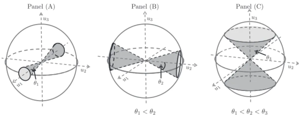
Figure 2. Geometric representation of PC directions in Example 1. The sphere represents the space of possible sample eigenvectors. Panel (A) shows that the first sample eigenvector tends to lie in the dark gray cone, with the θ1 angle. Similarly, Panels (B) and (C) show that the second and the third
sample eigenvectors respectively tend to lie in the dark gray cones, whose angles are θ2 andθ3. Note that θ1 is less than θ2, which is again less than
θ3.
dimension and the product of the sample size with the spike size. When this ra-tio converges to a nonzero constant, the sample eigenvector converges to a cone, with a certain angle to its corresponding population eigenvector. In the HDLSS case, the angle between the sample eigenvector and its population counterpart converges to a limiting distribution. Several generalizations of the multi-spike covariance models are also explored, and additional theoretical results are pre-sented.
We first introduce two examples to help understand the asymptotic results of conical structure for sample eigendirections.
Example 1 (Multiple-component spike models with distinguishable
eigenval-ues). Let X1, . . . , Xn be random sample vectors according to (4.2), where the
population eigenvalues satisfy, asn, d→ ∞,
λ1> λ2 > λ3≫λ4=· · ·=λd= 1, d nλj → cj, j = 1,2,3, with 0≤c1< c2< c3≤ ∞.
In Figure 2, the sphere represents the space of all possible sample eigen-directions, with the first three population eigenvectors as the coordinate axes. From Theorem 3, as n, d → ∞, the sample eigenvector ˆu1 lies in the dark
gray cone, shown in Panel (A) of Figure 2, with the angle of the cone θ1 =
Figure 3. Example 1: Simulated angles between sample and population eigenvectors. Panel (A) shows realizations of angles between sample and population eigenvectors as black gray dots (black is first, dark gray is second, light gray is third). Distributions are studied using kernel density estimates, and compared with the theoretical valuesθj forj= 1,2,3, shown as dashed lines. Panel (B) studies randomness of eigen-directions within the cones shown in Figure 2, by showing the distribution of pairwise angles between realizations of the sample eigenvectors. All 3 colors are overlaid here, and all angles are close to 90 degrees, which is consistent with the randomness of the respective sample eigenvectors within the cones.
respectively, lie in the dark gray cones, shown in Panels (B) and (C) of Fig-ure 2, with angles θ2 = arccos(1/
√
1 +c2) and θ3 = arccos(1/
√
1 +c3). For
c1 < c2 < c3, we have θ1< θ2 < θ3, as shown in Figure 2.
Our Proposition S4.1 in the supplementary material includes the two bound-ary cases studied by Shen, Shen, and Marron (2012b) as special cases. When
c1 = c2 = c3 = 0, it follows that θ1 = θ2 = θ3 = 0, in the domain of
consis-tency (Shen, Shen, and Marron (2012b)). When c1 = c2 = c3 = ∞, we have
θ1 = θ2 = θ3 = 90 degrees and strong inconsistency Shen, Shen, and Marron
(2012b).
We investigated convergence, using simulations, over a range of settings, with
n = 50, 100, 200, 500, 1,000, 2,000, where d/n = 50, and c1 = 0.2, c2 = 0.4,
c3 = 1. The full sequence, illustrating this convergence, is shown in Figure 3 A
of the supplementary material. Figure 3 shows the intermediate case ofn= 200. For one data set with this distribution, we computed angles between the sample and population eigenvectors. Repeating this procedure over 100 replications, we got 100 angles for each of the first three eigenvectors, shown as black, dark gray, and light gray points in Panel (A). The black, dark gray, light gray curves are the corresponding kernel density estimates. Panel (A) shows that the simulated angles close to the corresponding theoretical angles θj, j = 1,2,3, shown as
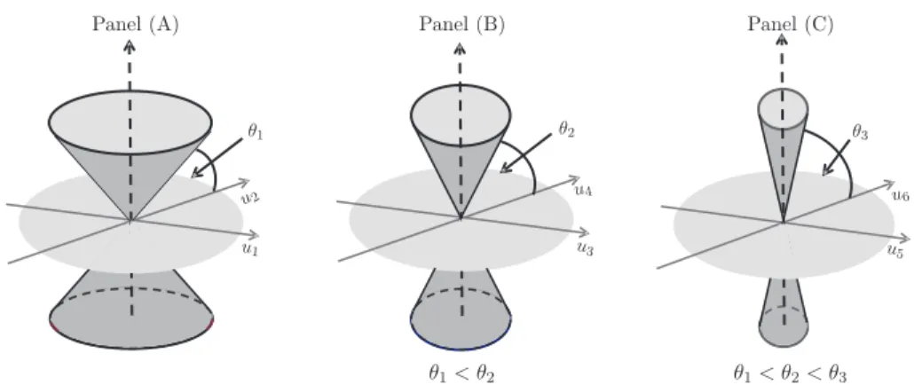
Figure 4. Example 2: Geometric representation of PC directions. Panel (A) shows the cone to which the first group of sample eigenvectors converge in the dark gray. This cone has angleθ1with the light gray subspace, generated by
the first group of population eigenvectors. Similarly, Panel (B) (Panel (C)) shows the cone to which the second (third) group of sample eigenvectors converges shown as a dark gray cone, which has angle θ2 (θ3) with the
subspace, generated by the second (third) group of population eigenvectors.
Panel (B) in Figure 3 studies randomness of eigen-directions within the cones shown in Figure 2. We calculated pairwise angles between realizations of the sam-ple eigenvectors for the three cones, showing angles and kernel density estimates using colors as in Panel (A) of Figure 3. All angles ware close to 90 degrees, consistent with randomness in high dimensions, see Hall, Marron, and Neeman (2005); Yata and Aoshima (2012a); Jung and Marron (2009); Jung, Sen, and Marron (2012); Cai, Fan, and Jiang (2013).
Example 2. (Multiple-component spike models with indistinguishable
eigenval-ues) Here we take the six leading population eigenvalues to satisfy, as n, d→ ∞
λ1 =λ2> λ3 =λ4> λ5 =λ6≫λ7=· · ·=λd= 1, d nλ2j−1 → cj, j= 1,2,3, with 0≤c1 < c2 < c3 ≤ ∞.
From Theorem 4, Panel (A) in Figure 4 shows, as a dark gray cone, the region where the first group of sample eigenvectors ˆu1and ˆu2lie in the limit asn, d→ ∞.
This has the angleθ1= arccos(1/
√
1 +c1) with the light gray subspace generated
by the first group of population eigenvectors, u1 and u2. Similarly, Panel (B)
(Panel (C)) presents, as a dark gray cone, the region where the second (third) group of sample eigenvectors ˆu3 and ˆu4 (ˆu5 and ˆu6) lie in the limit as n, d→ ∞.
This has the angle θ2 = arccos(1/
√
1 +c2) (θ3 = arccos(1/
√
1 +c3)) with the
subspace generated by the second (third) group of population eigenvectors, u3
Our Proposition S2.1 in the supplementary material includes boundary cases studied by Shen, Shen, and Marron (2012b) as special cases. For c1=c2=c3=
0, it follows that θ1 = θ2 = θ3 = 0, in the domain of subspace consistency; see
Theorem 4.3 of Shen, Shen, and Marron (2012b). Whenc1 =c2 =c3 =∞, we
have θ1 = θ2 = θ3 = 90 degrees and strong inconsistency; see Theorem 4.3 of
Shen, Shen, and Marron (2012b).
5.1. Growing sample size asymptotics
We now study asymptotic properties of PCA as n→ ∞. We consider multi-ple component spike models with distinguishable population eigenvalues in Sec-tion 5.1.1, and with indistinguishable eigenvalues in SecSec-tion 5.1.2. We vary d
from d ≪ n, through the random matrix version with d ∼ n, to the high di-mension medium sample size (HDMSS) asymptotics of Cabanski et al. (2010), Yata and Aoshima (2012b), and Aoshima and Yata (2015), with d≫ n → ∞. Aoshima and Yata (2015) improves the results of Yata and Aoshima (2012b) under mild conditions.
5.1.1. Multiple component spike models with distinguishable eigenvalues
We consider multiple component spike models where the population eigen-values satisfy the following.
A1. Asn, d→ ∞,λ1 >· · ·> λm≫λm+1 → · · · →λd= 1. A2. Asn, d→ ∞, nλd
j →cj, where 0< c1 <· · ·< cm <∞.
Here, that λ1 >· · · > λm makes it possible to separately consider the first
m principle component signals and their corresponding asymptotic properties. That λm ≫λm+1 → · · · →λd = 1 enables clear separation of the signal in the
first m components from the noise in the higher order components.
InA2, thepositiveandnegative information are of the same order: increasing
nand the spike positively impacts the consistency of PCA, whereas increasingd
has a negative impact.
In our context, we take H ={m+ 1, . . . , d} as the noise index set and the space spanned by the noise eigenvectors as
S= span{uj, j∈H}. (5.1)
For each sample eigenvector ˆuj,j ∈ H, we study the angle between ˆuj and the
space S, as defined in Jung and Marron (2009) and Shen, Shen, and Marron (2012b), and illustrated in Figure B of the supplementary material.
Theorem 3. Under Assumptions 1, A1, and A2, as n, d → ∞, the sample eigenvalues satisfy ˆ λj λj a.s −→1 +cj, 1≤j≤m, nλˆj dλj a.s −→1, m+ 1≤j ≤[n∧d], (5.2)
and the sample eigenvectors satisfy
|<uˆj, uj >| a.s −−→(1 +cj)−1/2, 1≤j≤m, |<uˆj, uj >|= Oa.s { (nd)1/2}, m+ 1≤j≤[n∧d], angle<uˆj,S>−−→a.s 0, m+ 1≤j≤[n∧d]. (5.3)
Remark 5. Thed/nλj →cj contains three scenarios: n, d, andλj → ∞;d, λj → ∞ and n < ∞ (HDLSS); n, d → ∞ and λj < ∞. We study the first two.
Theorem 3 studies the first scenario and Paul (2007) studied the third. The results in Paul (2007) are based on the normal assumption, unnecessary here, and do not pertain to indistinguishable eigenvalues.
Remark 6. The results of (5.2) and (5.3) suggest that, as the eigenvalue index increases, the proportional bias between the sample and population eigenvalue increases, so the angle between the sample and corresponding population eigen-vectors increases. This is because larger eigenvalues (i.e. with small indices) contain more positive information, which makes the corresponding sample eigen-values/eigenvectors less biased. These results are graphically illustrated in Figure 1 and empirically verified in Figure 2, for the specific model in Example 1. More empirical support is provided in the supplementary material.
Remark 7. Theorem 3 can be extended to include the random matrix and
HDMSS cases; This is shown in Section S4.1 of the supplementary material.
5.1.2. Multiple component spike models with indistinguishable eigen-values
We consider spike models with themleading eigenvalues grouped intor(≥1)
tiers, each of which contains all given eigenvalues that are either the same or have the same limit. Specifically, the first m eigenvalues are grouped into r tiers, in which there areqk eigenvalues in thekth tier such that
∑r
l=1ql=m. Letq0 = 0,
qr+1 =d−
∑r
l=1ql, and the index set of the eigenvalues in thekth tier be
Hk= {k−1 ∑ l=0 ql+ 1, k−1 ∑ l=0 ql+ 2, . . . , k−1 ∑ l=0 ql+qk } , k= 1, . . . , r+ 1. (5.4) We make these formal assumptions.
B1. The eigenvalues in the kth tier have the limit δk(>0): lim n,d→∞ λj δk = 1, j ∈Hk, k = 1, . . . , r. B2. The eigenvalues in different tiers have different limits:
asn, d→ ∞, δ1 >· · ·> δr≫λm+1→ · · · →λd= 1.
B3. The ratio between the dimension and the product of the sample size with eigenvalues in the same tier converges to a constant:
asn, d→ ∞, d nδk →
ck, with 0< c1 <· · ·< cr <∞.
Since the sample eigenvalues within the same tier can not be asymptotically identified, the corresponding sample eigenvectors are indistinguishable. For j ∈ Hk, in order to study the asymptotic properties of the sample eigenvector ˆuj,
we consider the angle between ˆuj and the subspace spanned by the population
eigenvectorsuj in the same tier,
Sk= span{uj, j ∈Hk}. (5.5)
Theorem 4. Under Assumptions 1, B1, B2, and B3, as n, d→ ∞, the sample eigenvalues satisfy ˆ λj λj a.s −→1 +ck, j∈Hk, k= 1, . . . , r, nλˆj dλj a.s −→1, m+ 1≤j≤[n∧d], (5.6)
and the sample eigenvectors satisfy
angle<uˆj,Sk> a.s −−→arccos{(1 +ck)−1/2 } , j∈Hk, k= 1, . . . , r, |<uˆj, uj >|= Oa.s { (nd)1/2}, m+ 1≤j≤[n∧d], angle<uˆj,Sr+1> a.s −−→1, m+ 1≤j≤[n∧d]. (5.7)
Theorem 4 extends Theorem 3. For higher-order eigenvalues, the sample eigenvalues are more biased, while the angles between the sample eigenvectors and the subspaces spanned by their population counterparts in the same tiers are larger. See Figure 3 for an illustration of the specific model considered in Example 2. Theorem 4 can be extended to cover the random matrix and HDMSS cases, see Section S4.2 of the supplementary material.
5.2. HDLSS asymptotics
We study the asymptotic properties of PCA in the HDLSS context. Here, the ratios between the sample eigenvalues and their population counterparts con-verge to non-degenerate random variables, as do the angles between the sample eigenvectors and the space spanned by the corresponding population eigenvec-tors.
Since the sample size is fixed, we can’t distinguish the two types of spike models considered in Sections 5.1.1 and 5.1.2. Hence, we merge the model as-sumptions there as follows.
C1. For fixedn, asd→ ∞,λ1 ≥ · · · ≥λm ≫λm+1→ · · · →λd= 1. C2. For fixedn, asd→ ∞,
d nλj →
cj, with 0< c1≤ · · · ≤cm<∞.
Now the sample eigenvalues and eigenvectors converge to non-degenerate random variables rather than constants. Consider the m × d matrix M = [C,0m×(d−m)]m×d, whereC= diag{c−
1/2 1 , . . . , c
−1/2
m }is anm×mdiagonal matrix
and 0m×(d−m) is them×(d−m) zero matrix. Take
Z = (zi,j)n×d and W =MZTZMT, (5.8)
wherezi,j is defined in (4.2).
Given a fixed sample size, the sample eigenvalues can’t be asymptotically distinguished, nor can the corresponding sample eigenvectors. To study the asymptotic behavior of the sample eigenvectors, we need to consider the spaceSk
spanned by the corresponding population eigenvectors, as defined in (5.5), with the index setsH1={1, . . . , m}and H2 ={m+ 1, . . . , d}.
Theorem 5. Under Assumptions 1, C1 and C2, for fixed n, as d → ∞, the
sample eigenvalues satisfy
ˆ λj λj a.s −→ cj nλj(W) +cj, 1≤j ≤m, nλˆj dλj a.s −→1, m+ 1≤j≤n, (5.9)
where W is defined in (5.8), and the sample eigenvectors satisfy
angle<uˆj,S1 >−−→a.s arccos
{( 1 +λ n j(W) )−1/2} , 1≤j≤m, |<uˆj, uj >|= Oa.s(d−1/2), m+ 1≤j≤n, angle<uˆj,S2 > a.s −−→1, m+ 1≤j≤n. (5.10)
Remark 8. Under the normal distribution, then Theorem 5 reduces to studies in Jung, Sen, and Marron (2012). Theorem 5 shows that the results in Jung, Sen, and Marron (2012) can be strengthened to almost sure convergence.
Remark 9. For 1 ≤ j ≤ m, as the relative size of the eigenvalue decreases,
the angle between ˆuj and S1 increases. However, this phenomenon is not as
strong as in the growing sample size settings studied in Section 5.1, where the sample eigenvectors can be separately studied, and the corresponding angles have a non-random increasing order.
Remark 10. AssumptionC2 can be relaxed to include boundary cases, in which
there exists an integerm0∈[1, m] such thatcm0 = 0, positive information
dom-inates in the leading m0 spikes, or cm0+1 =∞, negative information dominates
in the remaining high-order spikes. These results are presented in Section S5 of the supplementary material.
6. Proofs
We only present a detailed proof for Theorems 4. Theorem 3 is a special case of Theorem 4. The proof of properties of sample eigenvectors is in Section 6.1, while the properties of sample eigenvalues’ properties are shown in Section S6.1 of the supplementary material.
The proofs of Theorems 1, 2, and 5 are in Sections S6 and S7 of the sup-plementary material, which also contains proofs of extensions of Theorems 3, 4, and 5.
6.1. The proof of sample eigenvectors’ properties
This subsection gives the proof for the properties of the sample eigenvectors in Theorem 4.
The population eigenvalues are grouped into r + 1 tiers and Hk at (5.4) is
the index set of the eigenvalues in thekth tier. Let ˆ
uj= (ˆu1,j, . . . ,uˆd,j)T, j = 1, . . . , d and ˆUk,l= (ˆui,j)i∈Hk,j∈Hl, 1≤k, l≤r+ 1.
Then, the sample eigenvector matrix ˆU can be expressed as
ˆ U = [ˆu1,uˆ2, . . . ,uˆd] = ˆ U1,1 Uˆ1,2 · · · Uˆ1,r+1 ˆ U2,1 Uˆ2,2 · · · Uˆ2,r+1 .. . ... ... ˆ Ur+1,1Uˆr+1,2· · ·Uˆr+1,r+1 . (6.1)
Since uj = ej, j = 1, . . . , d, the inner product between the sample and
population eigenvectors satisfies
and the angle between the sample eigenvector and the corresponding population subspaceSk in (5.5) satisfies {cos [angle (ˆuj,Sk)]}2= ∑ l∈Hk ˆ u2l,j, k= 1, . . . , r+ 1. (6.2) We first state Bai-Yin’s law Bai and Yin (1993).
Lemma 1. Suppose B = (1/s)ZsT×mZs×m, where Zs×m is an s×m random matrix whose elements are i.i.d. and have zero mean, unit variance, and finite fourth moment. As s → ∞ and m/s → c ∈ [0,∞), the largest and smallest non-zero eigenvalues of B converge almost surely to (1 +√c)2 and (1−√c)2, respectively.
6.1.1. Asymptotic properties of the sample eigenvectors uˆj withj > m
We derive the asymptotic properties as follows. First, we show that asn, d→
∞, the angle between ˆuj and uj converges to 90 degrees: |<uˆj, uj >|2= ˆu2j,j = Oa.s
(n
d
)
, j=m+ 1, . . . ,[n∧d]. (6.3) We then show that, as n, d → ∞, the angle between ˆuj and the corresponding
subspaceSr+1 converges to 0, where Sr+1 is defined as in (5.5):
angle<uˆj,Sr+1 >−−→a.s 0, j=m+ 1, . . . ,[n∧d]. (6.4)
To account for the first step, let W = Λ−1/2UTUˆΛˆ1/2, where U and V are defined in (4.1) and ˆU and ˆΛ are defined in (4.4). It follows from (4.1), (4.2), and (4.4) thatW WT = (1/n)ZTZ, whereZ is defined in (5.8). Considering the
kth diagonal entry of the equivalent matricesW WT and (1/n)ZTZ, and noting thatwk,j =λ− 1/2 k λˆ 1/2 j uˆk,j (U =Id), it follows that λ−k1 d ∑ j=1 ˆ λjuˆ2k,j = d ∑ j=1 w2k,j = 1 n n ∑ i=1 zi,k2 . k= 1, . . . , d. (6.5) According to (6.5), we have ˆ u2j,j ≤ λm+1 ˆ λ[n∧d] ( 1 n n ∑ i=1 z2i,j ) , j =m+ 1, . . . ,[n∧d]. (6.6) Select the m+ 1th tonth columns of Z in (5.8) to form then×[n∧d] random matrix ¯Z. Note that ∑ni=1zi,j2 ,j=m+ 1, . . . ,[n∧d], are the diagonal elements of ¯ZTZ¯ and less than or equal to the largest eigenvalue of ¯ZTZ¯. Then it follows from (6.6) that
max m+1≤j≤[n∧d]uˆ 2 j,j ≤ λm+1 ˆ λ[n∧d] λmax( 1 nZ¯ TZ¯) (6.7)
which, together with the asymptotic properties of the sample eigenvalues (5.6) and Lemma 1, yields (6.3).
For the second step, according to (6.2) we need to show that
d
∑
k=m+1
ˆ
u2k,j−−→a.s 1, j=m+ 1, . . . ,[n∧d]. (6.8) The non-zero kth diagonal entry of WTW is between its smallest and largest eigenvalues. Since WTW shares the same non-zero eigenvalues as (1/n)ZZT, it
follows that, for j= 1, . . . ,[n∧d],
λmin(1 nZZ T)≤ˆλ j d ∑ k=1 λ−k1uˆ2k,j= d ∑ k=1 w2k,j≤λmax(1 nZZ T), (6.9)
which yields that, for j=m+ 1, . . . ,[n∧d],
λj ˆ λj λmin(1 nZZ T)≤ d ∑ k=1 λjλ−k1uˆ 2 k,j≤ λj ˆ λj λmax(1 nZZ T). (6.10)
According to Lemma 1 and the asymptotic properties of the sample eigenval-ues (5.6), we have that, for j=m+ 1, . . . ,[n∧d],
λj ˆ λj λmin ( 1 nZZ T ) and λj ˆ λj λmax ( 1 nZZ T ) a.s −−→1. (6.11) In addition, it follows from Assumption B2 that, for j=m+ 1, . . . ,[n∧d],
{
λjλ−k1 →0, k= 1, . . . , m,
λjλ−k1 →1, k=m+ 1, . . . d.
(6.12) Combining (6.10), (6.11), and (6.12), we have (6.8), which further leads to (6.4).
6.1.2. Asymptotic properties of the sample eigenvectors uˆj with
j∈[1, m]
We need to prove that, for j = 1, . . . , m, the angle between the sample eigenvector ˆuj and the corresponding population subspaceSl,j ∈Hl, converges
to arccos(1/√1 +cl),l= 1, . . . , r. According to (6.2), we only need to show that
∑ k∈Hl ˆ u2k,j −−→a.s 1 1 +cl , j ∈Hl, l= 1, . . . , r. (6.13)
We provide the detailed proof of (6.13) for l = 1, and briefly illustrate how repeating the same procedure can lead to (6.13) forl >2.
In order to show (6.13) for l = 1, we need a lemma about the asymptotic properties of the eigenvector matrix ˆU in (6.1):
Lemma 2. Under Assumptions in Theorem 4 and as n, d→ ∞, the rows of the eigenvector matrix Uˆ satisfy
r ∑ l=1 (1 +cl)chc−l 1 ∑ j∈Hl ˆ u2k,j−−→a.s 1, k∈Hh, h= 1, . . . , r, (6.14) and the columns of the eigenvector matrix Uˆ satisfy
r ∑ h=1 ∑ k∈Hh ˆ u2k,j −−→a.s 1 1 +cl , j∈Hl, l= 1, . . . , r. (6.15) In addition, we have r ∑ l=1 (1 +cl) ∑ j∈Hl ˆ u2k,j−−→a.s 1, k∈H1. (6.16)
Lemma 2 is proved in Section S6.4.3 of the supplementary material. We now show how to use Lemma 2 to prove (6.13) forl= 1. If h = 1 in (6.14), we have that ∑r l=1 (1 +cl)c1c−l 1 ∑ j∈Hl ˆ u2k,j −−→a.s 1, k∈H1. (6.17)
Note thatc1c−l 1 <1 for l >1, and comparing (6.16) with (6.17), we get that
r ∑ l=2 ∑ j∈Hl ˆ u2k,j −−→a.s 0, ∑ j∈H1 ˆ u2k,j −−→a.s 1 1 +c1 , k∈H1, (6.18)
which then yields that
∑ k∈H1 ∑ j∈H1 ˆ u2k,j−−→a.s q1 1 +c1 , (6.19)
whereq1is the number of eigenvalues inH1(5.4). Summing overj∈H1in (6.15),
we have that ∑r h=1 ∑ k∈Hh ∑ j∈H1 ˆ u2k,j −−→a.s q1 1 +c1 . (6.20)
It follows from (6.19) and (6.20) that
r ∑ h=2 ∑ k∈Hh ∑ j∈H1 ˆ u2k,j −−→a.s 0, (6.21) which, together with (6.15) forl= 1, yields
∑ k∈H1 ˆ u2k,j−−→a.s 1 1 +c1 , j ∈H1. This is (6.13) forl= 1.
We now prove (6.13) for l = 2, . . . , r. Note that it follows from (6.21) that (6.14) becomes r ∑ l=2 (1 +cl)chc−l 1 ∑ j∈Hl ˆ u2k,j−−→a.s 1, k∈Hh, h= 2, . . . , r. (6.22)
It follows from (6.18) that (6.15) becomes
r ∑ h=2 ∑ k∈Hh ˆ u2k,j−−→a.s 1 1 +cl , j∈Hl, l= 2, . . . , r. (6.23) Similar to (6.16), we have r ∑ l=2 (1 +cl) ∑ j∈Hl ˆ u2k,j −−→a.s 1, k∈H2. (6.24)
Combining (6.22), (6.23), and (6.24), we can prove (6.13) for l = 2. We can repeat the same procedure for l= 3, . . . , r.
Supplementary Materials
Additional results, simulations, and proofs can be found in the online sup-plementary materials.
Acknowledgements
This material was based upon work partially supported by the NSF grant DMS-1127914 to the Statistical and Applied Mathematical Science Institute. This work was partially supported by NIH grants MH086633, 1UL1TR001111, and MH092335, and NSF grants SES-1357666 and DMS-1407655. The content is solely the responsibility of the authors and does not necessarily represent the official views of the NIH.
References
Ahn, J., Marron, J. S., Muller, K. M. and Chi, Y.-Y. (2007). The high-dimension, low-sample-size geometric representation holds under mild conditions.Biometrika94, 760-766. Aoshima, M. and Yata, K. (2011). Two-stage procedures for high-dimensional data. Sequent.
Anal. 30, 356-399.
Aoshima, M. and Yata, K. (2015). Asymptotic normality for inference on multisample, high-dimensional mean vectors under mild conditions.Method. Comput. Appl. Probab.17, 419-439.
Bai, Z. and Silverstein, J. W. (2009).Spectral Analysis of Large Dimensional Random Matrices. Springer.
Bai, Z. D. and Yin, Y. Q. (1993). Limit of the smallest eigenvalue of a large dimensional sample covariance matrix.Ann. Probab.21, 1275-1294.
Beran, R. (1996). Stein estimation in high dimensions: a retrospective.Research Developments in Probability and Statistics: Madan L. Puri Festschrift, 91-110.
Beran, R. et al. (2010). The unbearable transparency of stein estimation. In Nonparametrics and Robustness in Modern Statistical Inference and Time Series Analysis: A Festschrift in honor of Professor Jana Jureckova, 25-34. Institute of Mathematical Statistics. Borysov, P., Hannig, J. and Marron, J. S. (2014). Asymptotics of hierarchical clustering for
growing dimension.J. Multivariate Anal. 124, 465-479.
Cabanski, C., Qi, Y., Yin, X., Bair, E., Hayward, M., Fan, C., Li, J., Wilkerson, M., Marron, J. S., Perou, C. and Hayes, D. (2010). Swiss made: standardized within class sum of squares to evaluate methodologies and dataset elements.PloS One5, e9905.
Cai, T., Fan, J. and Jiang, T. (2013). Distributions of angles in random packing on spheres.J. Mach. Learn. Res.14, 1837-1864.
Casella, G. and Hwang, J. T. (1982). Limit expressions for the risk of james-stein estimators. Canad. J. Statist.10, 305-309.
Chernozhukov, V., Chetverikov, D. and Kato, K. (2014). Central limit theorems and bootstrap in high dimensions. arXiv:1412.3661.
Denoeud, F., Aury, J.-M., Da Silva, C., Noel, B., Rogier, O., Delledonne, M., Morgante, M., Valle, G., Wincker, P., Scarpelli, C. et al. (2008). Annotating genomes with massive-scale rna sequencing.Genome Biol9, R175.
Fan, J. and Lv, J. (2008). Sure independence screening for ultrahigh dimensional feature space. J. Roy. Statist. Soc. Ser. B70, 849-911.
Ferraty, F. and Vieu, P. (2004). Nonparametric models for functional data, with application in regression, time series prediction and curve discrimination. Nonparametr. Statist.16, 111-125.
Hall, P., Marron, J. S. and Neeman, A. (2005). Geometric representation of high dimension, low sample size data.J. Roy. Statist. Soc. Ser. B67, 427-444.
Hellton, K. and Thoresen, M. (2014). Asymptotic distribution of principal component scores for pervasive, high-dimensional eigenvectors. arXiv preprint arXiv:1401.2781.
Johnstone, I. M. and Lu, A. Y. (2009). On consistency and sparsity for principal components analysis in high dimensions.J. Amer. Statist. Assoc.104, 682-693.
Jolliffe, I. (2005).Principal Component Analysis. Wiley Online Library.
Jung, S. and Marron, J. S. (2009). PCA consistency in high dimension, low sample size context. Ann. Statist.37, 4104-4130.
Jung, S., Sen, A. and Marron, J. S. (2012). Boundary behavior in high dimension, low sample size asymptotics of PCA.J. Multivariate Anal.109, 190-203.
Kimes, P. K. and Cabanski, C. R. (2013). Sigfuge (tutorial).
Lee, S., Zou, F. and Wright, F. A. (2010). Convergence and prediction of principal component scores in high-dimensional settings.Ann. Statist.38, 3605-3629.
Liu, Y., Hayes, D. N., Nobel, A. and Marron, J. S. (2008). Statistical significance of clustering for high-dimension, low sample size data.J. Amer. Statist. Assoc.103, 1281-1293. Marcenko, V. A. and Pastur, L. A. (1967). Distribution of eigenvalues for some sets of random
matrices.Sbornik: Mathematics1, 457-483.
Marron, J. S. and Alonso, A. M. (2014). An overview of object oriented data analysis.Biometr. J. 56, 732-753.
Murillo, F. et al. (2008). The incredible shrinking world of DNA microarrays.Molecular BioSys-tems4, 726-732.
Paul, D. (2007). Asymptotics of sample eigenstructure for a large dimensional spiked covariance model.Statist. Sinica17, 1617-1642.
Paul, D. and Johnstone, I. (2007). Augmented sparse principal component analysis for high-dimensional data. Technical Report, UC Davis.
Portnoy, S. (1984). Asymptotic behavior of m-estimators of p regression parameters whenp2/n
is large. i. consistency.Ann. Statist.12, 1298-1309.
Portnoy, S. et al. (1988). Asymptotic behavior of likelihood methods for exponential families when the number of parameters tends to infinity.Ann. Statist.16, 356-366.
Ramsay, J. O. (2005).Functional Data Analysis. Wiley Online Library.
Ramsay, J. O. and Silverman, B. W. (2002). Applied Functional Data Analysis: Methods and Case Studies. Springer New York.
Rollin, A. (2013). Stein’s method in high dimensions with applications. arXiv:1101.4454. Shen, D., Shen, H. and Marron, J. S. (2012a). Consistency of sparse PCA in high dimension,
low sample size contexts.J. Multivariate Anal.115, 317-333.
Shen, D., Shen, H. and Marron, J. S. (2012b). A general framework for consistency of principal component analysis.arXiv:1211.2671.
Stein, C. (1956). Inadmissibility of the usual estimator for the mean of a multivariate normal distribution. In Proceedings of the Third Berkeley Symposium on Mathematical Statistics and Probability1, 197-206.
Tracy, C. A. and Widom, H. (1996). On orthogonal and symplectic matrix ensembles. Commu-nications in Mathematical Physics177, 727-754.
Wang, H. and Marron, J. S. (2007). Object oriented data analysis: Sets of trees.Ann. Statist. 35, 1849-1873.
Wilhelm, B. T. and Landry, J.-R. (2009). RNA-seq-quantitative measurement of expression through massively parallel RNA-sequencing.Methods48, 249-257.
Yata, K. and Aoshima, M. (2009). PCA consistency for non-gaussian data in high dimension, low sample size context.Comm. Statist. Theory Methods38, 2634-2652.
Yata, K. and Aoshima, M. (2010a). Effective PCA for high-dimension, low-sample-size data with singular value decomposition of cross data matrix. J. Multivariate Anal.101, 2060-2077.
Yata, K. and Aoshima, M. (2010b). Intrinsic dimensionality estimation of high-dimension, low sample size data with d-asymptotics.Comm. Statist. Theory Methods39, 1511-1521. Yata, K. and Aoshima, M. (2012a). Effective PCA for high-dimension, low-sample-size data
with noise reduction via geometric representations.J. Multivariate Anal.105, 193-215. Yata, K. and Aoshima, M. (2012b). Inference on high-dimensional mean vectors with fewer
ob-servations than the dimension. Methodology and Computing in Applied Probability 14, 459-476.
Yata, K. and Aoshima, M. (2013). PCA consistency for the power spiked model in high- dimen-sional settings.J. Multivariate Anal.122, 334-354.
Interdisciplinary Data Sciences Consortium, Department of Mathematics and Statistics, Uni-versity of South Florida, Tampa, FL, 33620, USA.
E-mail: [email protected]
School of Business, University of Hong Kong, Pokfulam, Hong Kong. E-mail: [email protected]
Department of Biostatistics and Biomedical Research Imaging Center, University of North Car-olina at Chapel Hill, Chapel Hill, NC 27599, USA.
E-mail: [email protected]
Department of Statistics and Operations Research, University of North Carolina at Chapel Hill, Chapel Hill, NC 27599, USA.
E-mail: [email protected]