E4D: A distributed memory parallel electrical geophysical modeling and inversion code

PNNL-SA-23783

E4D: A distributed memory

parallel electrical geophysical

modeling and inversion code

User Guide - Version 1.0

September 2014

E4D: A distributed memory parallel electrical geophysical modeling and inversion code Copyright © 2014, Battelle Memorial Institute

All rights reserved.

1. Battelle Memorial Institute (hereinafter Battelle) hereby grants permission to any person or entity lawfully obtaining a copy of this software and associated documentation files (hereinafter “the Software”) to redistribute and use the Software in source and binary forms, with or without modification. Such person or entity may use, copy, modify, merge, publish, distribute, sublicense, and/or sell copies of the Software, and may permit others to do so, subject to the following conditions:

 Redistributions of source code must retain the above copyright notice, this list of conditions and the following disclaimers.

 Redistributions in binary form must reproduce the above copyright notice, this list of conditions and the following disclaimer in the documentation and/or other materials provided with the distribution.  Other than as used herein, neither the name Battelle Memorial Institute or Battelle may be used in any

form whatsoever without the express written consent of Battelle.

 Redistributions of the software in any form, and publications based on work performed using the software should include the following citation as a reference:

Johnson, T. C., R. J. Versteeg, A. Ward, F. D. Day-Lewis, and A. Revil (2010), Improved hydrogeophysical characterization and monitoring through parallel modeling and

inversion of time-domain resistivity and induced polarization data, Geophysics, 75(4), Wa27-Wa41.

2. THIS SOFTWARE IS PROVIDED BY THE COPYRIGHT HOLDERS AND CONTRIBUTORS "AS IS" AND ANY EXPRESS OR IMPLIED WARRANTIES, INCLUDING, BUT NOT LIMITED TO, THE IMPLIED WARRANTIES OF MERCHANTABILITY AND FITNESS FOR A PARTICULAR PURPOSE ARE DISCLAIMED. IN NO EVENT SHALL BATTELLE OR CONTRIBUTORS BE LIABLE FOR ANY DIRECT, INDIRECT, INCIDENTAL, SPECIAL, EXEMPLARY, OR CONSEQUENTIAL DAMAGES (INCLUDING, BUT NOT LIMITED TO, PROCUREMENT OF SUBSTITUTE GOODS OR SERVICES; LOSS OF USE, DATA, OR PROFITS; OR BUSINESS INTERRUPTION) HOWEVER CAUSED AND ON ANY THEORY OF LIABILITY, WHETHER IN CONTRACT, STRICT LIABILITY, OR TORT

(INCLUDING NEGLIGENCE OR OTHERWISE) ARISING IN ANY WAY OUT OF THE USE OF THIS SOFTWARE, EVEN IF ADVISED OF THE POSSIBILITY OF SUCH DAMAGE.

PNNL-SA-23783

E4D: A distributed memory parallel

electrical geophysical modeling and

inversion code

TC Johnson

September 2014

Prepared for

the U.S. Department of Energy

under Contract DE-AC05-76RL01830

Pacific Northwest National Laboratory

Richland, Washington 99352

Acknowledgments

E4D development was jointly funded by the U.S. Department of Energy - Office of Environmental Management and Office of Science, and the U.S. Department of Defense under the Environmental

Security Technology and Certification Progam. Development of the infrastructure modeling and inversion modeling capabilities was funded by the Pacific Northwest National Laboratory, with support for testing provided by the U.S. Department of Energy - Office of River Protection.

Contents

Acknowledgments ... iii 1.0 Overview ... 1.1 2.0 General Capability Description ... 2.1 3.0 Installation ... 3.1 3.1 Linux Installation ... 3.1 3.2 Windows Compilation... 3.1 3.3 Custom Compilation ... 3.3 4.0 Running e4d ... 4.1 4.1 Standard Execution ... 4.1 4.2 Batch Submission ... 4.1 5.0 Mode 1: ER Mesh Generation Mode ... 5.1 5.1 Introduction ... 5.1 5.2 Run Configuration File: e4d.inp ... 5.1 5.3 Mesh Files ... 5.2 5.4 Elements and Zones ... 5.3 5.5 Nodes and Boundaries ... 5.3 5.6 Mesh Configuration File ... 5.3 5.6.1 General Block ... 5.3 5.6.2 Control Points Block ... 5.4 5.6.3 Internal Boundary Configuration Block ... 5.6 5.6.4 Hole Configuration Block ... 5.8 5.6.5 Zone Configuration Block ... 5.8 5.6.6 Visualization Options Block ... 5.9 5.7 ER Mesh Generation Tutorial 1.1: Two Buried Blocks ... 5.9 5.7.1 Conceptual Diagram ... 5.9 5.7.2 Building the Mesh ... 5.10 5.7.3 Two_Block Mesh Visualization ... 5.11 5.7.4 Mesh Configuration File: two_blocks.cfg ... 5.11 5.8 ER Mesh Generation Tutorial 1.2: Buried Metallic Box, Sheet, and Line... 5.15 5.8.1 Overview ... 5.15 5.8.2 Conceptual Diagram ... 5.15 5.8.3 Building the mbsl Mesh ... 5.16 5.8.4 mbsl Mesh Visualization ... 5.17 5.8.5 Mesh Configuration File: mbsl.cfg ... 5.18 6.0 Mode 2: ER Forward Run Mode ... 6.1 6.1 Introduction ... 6.1

6.2 File Format for e4d.inp... 6.2 6.3 Analytic Solutions ... 6.2 6.4 Numeric Solutions ... 6.2 6.5 Mode 1 Reporting and Output ... 6.3 6.5.1 Screen Output ... 6.3 6.5.2 E4D Log File: e4d.log ... 6.3 6.5.3 Simulated Data and Survey File ... 6.3 6.5.4 Potential Files ... 6.3 6.6 ER Forward Run Tutorial 2.1: Two Buried Blocks ... 6.4 6.6.1 Overview ... 6.4 6.6.2 Using Mode 2 to Investigate Numeric Solution Accuracy ... 6.4 6.6.3 Survey File: two_blocks.srv ... 6.5 6.6.4 Output Options File: two_blocks.out ... 6.5 6.6.5 Mode 2 e4d.inp ... 6.6 6.6.6 Analytic Simulation ... 6.6 6.6.7 Numeric Simulation ... 6.8 6.6.8 Simulating a Survey and Viewing a Potential Field ... 6.9 6.7 ER Forward Run Tutorial 2.2: Buried Metallic Box, Sheet, and Line ... 6.10 6.7.1 Overview ... 6.10 6.7.2 Survey File: mbsl.srv ... 6.12 6.7.3 Potential Distributions for Measurement 2071 and 2072 ... 6.12 7.0 Mode 3: ER static inversion mode... 7.1 7.1 Overview ... 7.1 7.2 File Format for e4d.inp... 7.1 7.3 Mode 3 Inversion Options File ... 7.2 7.4 Structural Metric Codes ... 7.5 7.5 Weighting Function Codes ... 7.6 7.6 Example Constraints for Static Inversions ... 7.8 7.6.1 Smoothness Constrained Inversion ... 7.9 7.6.2 Smoothing with Sharp Boundaries (Blocky Inversion)... 7.9 7.6.3 Minimum Conductivity ... 7.10 7.6.4 Maximum Conductivity ... 7.11 7.6.5 Known Value with Uncertainty ... 7.11 7.7 Reporting ... 7.12 7.7.1 e4d.log File ... 7.12 7.8 ER Inversion Example 3.1: Imaging Two Blocks ... 7.14 7.8.1 Overview ... 7.14 7.8.2 Smoothness Constrained Inversion ... 7.16 7.8.3 Smoothness Constrained Inversion + Minimum Conductivity Constraint ... 7.21

7.8.4 Blocky Inversion ... 7.23 7.8.5 Discrete Value Inversion ... 7.26 7.9 ER Inversion Example 3.2: Imaging in the Presence of Buried Metal ... 7.29 7.9.1 Overview ... 7.29 7.9.2 Conceptual Model and Forward Simulation ... 7.29 7.9.3 Forward Mesh Generation ... 7.30 7.9.4 Generating a Custom Conductivity Distribution Outside of E4D ... 7.32 7.9.5 Synthetic Survey File Generation... 7.33 7.9.6 Smoothness Constrained Inversion ... 7.34 7.9.7 Anisotropic Weighting and Inequality Constraints ... 7.37 8.0 Mode 4: ER Time-Lapse Inversion Mode ... 8.1 8.1 Overview ... 8.1 8.2 File Format for e4d.inp... 8.1 8.3 Time-Lapse Survey List File Format ... 8.3 8.4 Mode 4 Inversion Options File ... 8.3 8.5 Example Time-Lapse Inversion Constraints ... 8.3 8.5.1 Spatially Smoothing the Transient Change in Conductivity ... 8.3 8.5.2 Transient Smoothing with Sharp Boundaries ... 8.4 8.6 Notes on Time-Lapse Inversion ... 8.5 8.7 Reporting ... 8.6 9.0 ER Time-Lapse Inversion Tutorial 4.1: Sinking Plume ... 9.1 9.1 Forward Modeling ... 9.2 9.1.1 Generating the Forward Modeling Mesh ... 9.2 9.1.2 Generating the Time-Lapse Conductivity Distributions ... 9.3 9.1.3 Synthetic Survey Generation ... 9.4 9.1.4 Generating the Inversion Mesh ... 9.4 9.1.5 Baseline Inversion ... 9.5 9.2 Time-Lapse Inversions Using the Baseline Solution as Reference ... 9.7 9.3 Time-Lapse Inversions Using the Previous Solution as Reference ... 9.9 10.0 bx Utility Program ... 10.12 Appendix A File Formats ... A.1

Figures

5.1. Diagram of the three types of control points used to define a mesh ... 5.5 5.2. Control point and zone map for mesh configuration file two_blocks.cfg. ... 5.10 5.3. A) Oblique view of mesh show outer boundaries of zone 4 and inner refined region

comprising the electrodes and box bounded by zone 1. ... 5.11 5.4. Conceptual diagram of surface electrodes with a subsurface containing an infinite

conductivity box, sheet, and line embedded in a background medium with a conductivity of 0.002 S/m ... 5.16 5.5. Cut-out view of the mbsl mesh showing nodes added by tetgen for the three infinite

conductivity boundaries ... 5.17 6.1. Zones 1-3 of computational mesh and electrode locations for the homogeneous

conductivity case ... 6.4 6.2. Zones 1-3 of computational mesh and electrode locations with blocks of anamolous

conductivity ... 6.9 6.3. Example numerical potential distributions generated for A) a homogeneous halfspace and

B) a heterogeneous halfspace with two blocks of anomalous conductivity ... 6.10 6.4. Cut-out view of the mbsl mesh showing nodes added by tetgen for the three infinite

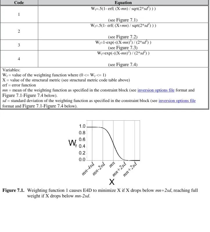
conductivity boundaries ... 6.11 6.5. Simulated potential isosurfaces for measurement A) 2071 and B) 2072 ... 6.13 7.1. Weighting function 1 causes E4D to minimize X if X drops below mn+2sd, reaching full

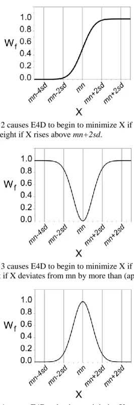
weight if X drops below mn-2sd. ... 7.7 7.2. Weighting function 2 causes E4D to begin to minimize X if the value of X rises above

mn-2sd, reaching full weight if X rises above mn+2sd. ... 7.8 7.3. Weighting function 3 causes E4D to begin to minimize X if the value of X deviates from

mn, reaching full weight if X deviates from mn by more than (approximately) 2sd. ... 7.8 7.4. Weighting function 4 causes E4D to begin to minimize X as the values of X approaches

mn, reaching full weight when X is equal to mn. ... 7.8 7.5. True subsurface conductivity distribution ... 7.15 7.6. Cut-out view of the inversion mesh, which is refined around electrodes anddoes not

include the block boundaries, and is coarser than the forward modeling mesh (Figure 6.2). ... 7.16 7.7. VisIt visualization of the smoothness constrained inversion results ... 7.21 7.8. Results of the smoothness constrained inversion with a minimum conductivity constraint

provides a slight improvement in resolution over the inversion without the minimum conductivity constraint (Figure 7.7). ... 7.23 7.9. Blocky inversion results display a significant improvement in resolution and converge in

approximately 50% of the time required for the smoothness constrained inversions. ... 7.26 7.10. Constrained value inversion, whereby the inversion is constrained to produce a solution

with only 3 conductivity values (0.002, 0.02, and 0.2 S/m). ... 7.28 7.11. Conceptual model conductivity distribution ... 7.30 7.12. Cut-out view of zone 1 of the forward modeling mesh ... 7.31

7.13. VisIt visualization of the true conductivity distribution representing the conceptual model in Figure 7.11. ... 7.32 7.14. Cut-out view of the inversion mesh mbsl_inv.1* . ... 7.35 7.15. Three different VisIt visualizations of the smoothness constrained inverse solution. ... 7.37 7.16. Three visualization of the inversion with anisotropic smoothing and upper and lower

conductivity boundary constraints. ... 7.39 9.1. Conceptual model of a spherical conductivity anomaly moving downward at 0.5 m per

time step in a background medium of 0.001 S/m. ... 9.2 9.2. Zone 1 of the forward modeling mesh. ... 9.3 9.3. Synthetic conductivity distribution at several depths. ... 9.4 9.4. Zone 1 of the inversion mesh ... 9.5 9.5. Baseline inversion conductivities range from approximately 0.0008 to 0.0012 S/m,

bounding the true conductivity of 0.001 S/m. ... 9.7 9.6. Comparison between true conductivity and imaged conductivity using the baseline

solution and previous solutions as the reference model with transient smoothing

constraints (structural metric 8). ... 9.11 A.1. Weighting function 1 causes E4D to begin to minimize X if the value of X drops below

mn+2sd, reaching the full wieight if X drops below mn-2sd ... A.8 A.2. Weighting function 2 causes E4D to begin to minimize X if the value of X rises above

mn-2sd, reaching the full wieight if X rises above mn+2sd ... A.9 A.3. Weighting function 3 causes E4D to begin to minimize X if the value of X deviates from

mn, reaching the full wieight if X deviates from mn more than (approximately) 2sd ... A.9 A.4. Weighting function 4 causes E4D to begin to minimize X as the value of X approaches

1.0

Overview

E4D is a three-dimensional (3D) modeling and inversion code designed for subsurface imaging and monitoring using static and time-lapse 3D electrical resistivity (ER) or spectral induced polarization (SIP) data. To address the computational demands of inverting large scale 3D and 4D data sets, E4D was designed specifically to run on distributed memory parallel high performance computing systems. However, E4D will run on any system with at least two processing cores.

E4D executes by reading a number of user-created ascii text input files, executing a particular run mode (e.g., mesh generation, ER forward simulation, ER inversion, SIP inversion), and reporting results. Run-time options made available through input files are designed to enable flexibility and a high level of customization for a particular problem, making E4D suitable for both advanced research applications, as well as more common applications.

A critical component of E4D is visualization. The E4D distribution includes the utility program bx,

which places E4D simulation results into an EXODUS II finite element data model formatted file. EXODUS II files are then visualized using the VisItvisualization program, an open source visualization code developed by the Lawrence Livermore National Laboratory. However, all of the files necessary for users to develop and operate other visualization codes are provided by E4D. Guidance concerning the use of VisIt is provided on the VisIt website, and is not included in this user guide.

The intended audience for this user guide includes researchers and other practitioners familiar with electrical geophysical methods and deterministic geophysical inversion. Guidance is given herein concerning how to enable and use the capabilities provided by E4D, with specific examples illustrated in a series of tutorials at the end of each chapter. Justifications for using a particular approach or capability are left to the user.

2.0

General Capability Description

E4D executes according to one of several run modes chosen by the user. Run modes can be classified generally as mesh generation modes, forward run modes, static inversion modes, and time-lapse inversion modes. Required input files, and the formats of those files, vary somewhat depending on the run mode. This user guide is divided into chapters that describe input file and other requirements specific to each run mode, including tutorials designed to illustrate the general use for each mode. The run modes are as follows:

Run Mode Function Description

1 ER Mesh Generation

Mode Mesh generation for electrical resistivity modeling and inversion 2 ER Forward Run Mode Direct current potential field and electrical resistivity survey simulation 3 ER Static Inversion

Mode Electrical resistivity inversion for a single survey 4 ER Time-lapse

Inversion Mode Electrical resistivity inversion for multiple time-lapse surveys 21* SIP Mesh Generation

Mode

Mesh generation for spectal induce polarization modeling and inversion

22* SIP Forward Run Mode

Complex potential field and spectral induced polarization survey simulation

23* SIP Static Inversion

Mode Spectral induced polarization inversion for a single survey 31* ER Tank Mesh

Generation Mode

Mesh generation for electrical resistivity modeling and inversion within a tank

32* ER Tank Forward Run Mode

Direct current potential field and electrical resistivity survey simulations for tank scale imaging

33* ER Tank Static

Inversion Mode Electrical resistivity inversion for a single survey within a tank 34* ER Tank Time-lapse

Inversion Model

Electrical resistivity inversion for multiple time-lapse surveys within a tank

41* SIP Tank Mesh Generation Mode

Mesh generation for spectral induced polarization modeling and inversion within a tank

42* SIP Tank Forward Run Mode

Complex potential field and spectral induced polarization survey simulations for tank scale imaging

43* SIP Tank Static Inversion Mode

Spectral induced polarization inversion for a single survey within a tank

* Not provided in the open source version of E4D

E4D provides conditional solution constraint options using the method of Iteratively Reweighted Least Squares (IRLS). Model constraint options are intended to be flexible, providing users numerous options for incorporating a priori information into the inverse problem, thereby improving imaging resolution (Johnson, submitted). In addition, E4D executes on an unstructured tetrahedral mesh, enabling users to accurately incorporate complex subsurface structures with known dimension and location. Each of the forward run and inversion modes has the optional capability of modeling the effects of metallic inclusions with arbitrary shape and size, including non-point electrodes, and accounting for (and

removing) those effects in the inversion. The module providing this capability is the Infrastructure Modeling and Inversion (IMI) module, and is not included as part of the open source distribution. Information concerning the availability of E4D capabilities that are not provided in the open source release version can be found on the E4D website at https://e4d.pnnl.gov .

3.0

Installation

Most distributed memory high performance computing systems operate on Unix/Linux-based operating systems. Because such systems vary in configuration, users will need to compile E4D for each individual system. E4D is provided with an installation script designed to automatically download missing software libraries and compile all of the components necessary to execute E4D in parallel. This includes the E4D executable e4d, the Message Passing Interface executable mpirun, the open source mesh generation programs triangle and tetgen, and the utility program bx. Because E4D downloads missing libraries, an internet connection is required for compilation. VisIt binaries are available for several operating systems, and must be downloaded separately. E4D requires the fortran90/95 compiler gfortran, which is freely available for Unix/Linux operating systems. Other fortran90/95 compilers may be used by modifying the make files provided with the E4D distribution. Also, E4D requires compilation on a 64-bit architecture.

3.1

Linux Installation

1. Download the E4D tarball from https://e4d.pnnl.gov 2. Extract E4D and third party codes:

tar -xzvf e4d_qc.tgz

This will unpack the directory e4d_qc. 3. Goto the directory e4d_qc/src.

4. Execute the build script build.bsh script with: ./build.bsh

The script build.bsh will compile and install the third party libraries necessary to build E4D (except

gfortran) and E4D utility programs including triangle, tetgen, petsc, netcdf, and exodus. Executables necessary to run E4D are copied to e4d_qc/bin, including:

 triangle: triangular mesh generation software used by E4D to build the surface boundary of the computational mesh,

 tetgen: tetrahedral mesh generation software used by E4D to build the unstructured computation mesh,

 bx: E4D utility file used to insert simulation and inversion results into an exodus file for visualization,

 mpirun: script used to call E4D with an allocation of processors, and

 e4d: main E4D program.

3.2

Windows Compilation

Compiling E4D on Windows requires the cygwin package, and is somewhat more involved than compiling on a linux/unix operating system. Cygwin is a collection of tools and libraries that enable linux

functionality on a windows operating system. E4D is provided with a set of bash scripts and make files that are used to compile E4D with cygwin in the same manner as the linux compilation described above.

To install cygwin, download the appropriate cygwin install script from

https://cygwin.com/install.html (note the 64-bit version is required for E4D). Review the installation instructions and execute the install script. The script will initiate a graphical user interface (gui) that provides options for the installation directory, the website from which to download packages and libraries, and a list of optional packages to install. For the installation directory, choose a directory without spaces in the name, (i.e., C:\cygwin). E4D requires (at a minimum) the following packages to be installed with cygwin:

 gcc-core

 gcc-fortran

 gcc-g++

 make - the GNU version of the make utility

 diffutils

 netcdf-fortran

 netcdr-fortran-devel

 python

Each of these packages can be located by entering the package names given above in the search dialog box of the package selection section of the installation gui. After choosing the packages, the installation script indicates a list of dependencies necessary for the selected list. Simply click “next” to accept the dependencies and begin the installation. When the cygwin installation completes, the install script will ask whether a cygwin icon should be place on the desktop or start menu. Choose one or both of these to simplify initiating the cygwin terminal window.

 Once cygwin is installed, download the E4D tarball from https://e4d.pnnl.gov into your cygwin home directory. For example, if cygwin was installed in C:/cygwin, your home directory is located in C:\cygwin\home\<your_user_name>.

 Open a cygwin terminal by double-clicking the icon cygwin created during installation (either on your start menu or desktop or both). If you are unfamiliar with the linux terminal window, it is similar to the dos command prompt. You should automatically be in your home directory within the terminal when it is opened.

 Decompress the E4D tarball by typing "tar -xvzf e4d_qc.tgz"

 Within the terminal, go to the directory <e4d_dir>/eq4_qc/src, where <e4d_dir> is the directory created from which the tarball was decompressed in the previous step.

 The cygwin build script is located in <e4d_dir>/e4d_qc/src/build_cygwin.bsh. To execute the build script, type "./build_cygwin.bsh" from on the cygwin command line.

At this point the build script will download and compile the required third party libraries, utility routines, and the e4d executable, and place them in <e4d_dir>/e4d_qc/bin.

Add the following lines to the file .bashrc, which is located in your home directory. alias ls='ls -l -hF --color=tty'

alias mpirun="<e4d_dir>/e4d_qc/third_party/petsc-3.4.3/arch-mswin-c-opt/bin/mpirun" export PATH=$PATH:<e4d_dir>/e4d_qc/ bin

Now type the command "source ~/.bashrc" from the cygwin terminal. Each of the programs necessary to execute e4d should now be visible from the command line, and will be visible with each new initiation of a cygwin terminal.

Note that all of the files necessary to execute e4d may be created using windows tools and file managers. However, all e4d programs described in the forthcoming documentation must be executed as described from the cygwin terminal command line. Visualization may then be conducted with the windows version of VisIt, downloadable from the VisIt website.

Note that some windows text editing programs leave hidden characters that corrupt ascii files as far as cygwin is concerned. It is important to use a linux compatible text editor when creating e4d input

files. TextPad is one example of a compatible text editor.

3.3

Custom Compilation

Many Linux-based high performance computing systems provide customized libraries, conveniently loaded and made available as modules. Because the compilation process on such systems varies, no specific instruction for compilation is given herein. However, the commands found in the build script (build.bsh) and corresponding make files provide information concerning which compilers and libraries are needed for each program.

4.0

Running e4d

4.1

Standard Execution

E4D is executed from the command line by typing:

<e4d_dir>/e4d_qc/bin/mpirun -np <num_proc> <e4d_dir>/e4d_qc/bin/e4d

where <e4d_dir> is the directory containing E4D (i.e. e4d_qc), and num_procis the number of processors

e4d will use during execution. Alternatively, <e4d_dir>/e4d_qc/bin can be placed in the executable path so that E4D is called by:

mpirun -np <num_proc> e4d

Note that some systems install a version of MPI by default, and set system variables so that

the mpirun command defaults to the version installed by the system. It is important to ensure that E4D is called using <e4d_dir>/e4d_qc/bin/mpirun so that the correct run-time libraries are used.

Upon execution, E4D will read the file e4d.inp to obtain the names of other input files and run instructions chosen by the user, all of which are described in the forthcoming documentation for each run mode.

4.2

Batch Submission

Most high performance computing systems use batch submission software to queue and prioritize parallel computation jobs. Job submission scripts and associated commands are system independent. Users should refer to system documentation and/or administrative help to run e4d in batch submission mode.

5.0

Mode 1: ER Mesh Generation Mode

5.1

Introduction

Mesh generation refers to the process E4D uses to generate the unstructured tetrahedral computational mesh used in forward and inverse simulations. Depending on user input, E4D can create a mesh that conforms to known subsurface boundaries such as borehole boundaries, water table boundaries, or the boundaries of buried tanks and other structural features. E4D can also create distinct zones within the mesh, which are the primary units whereby model constraints are defined to regularize or otherwise inform the inverse problem. Known boundaries incorporated into the mesh facilitate accurate ER and SIP data simulation in forward modes, and inform the inverse operation in inverse modes.

To create the mesh, E4D:

1. reads mesh construction options from a user supplied mesh configuration file, 2. builds an input file for the third party open source program triangle,

3. calls triangle to construct a high quality triangular mesh that will be used to define the surface boundary of the tetrahedral mesh,

4. loads the surface mesh constructed by triangle,

5. builds an input file for the open source tetrahedral mesh generator tetgen, 6. calls tetgen to build the tetrahedral mesh, and

7. if directed in the mesh configuration file, calls bx to build the exodus file used for mesh visualization.

5.2

Run Configuration File: e4d.inp

Upon execution, e4d reads the instructions provided in the run configuration file e4d.inp in order to determine which mode to run and which input files should be used to execute that mode. In ER mesh generation mode (mode 1), e4d.inp requires only two lines of instruction as described below, where each line in the table represents a line in the text file, as follows:

Input Description

1 Run Mode

mesh_configuration_filename Name of the mesh configuration file

The mesh configuration file (described below) name must end with the suffix .cfg, which E4D uses to delineate between mesh configuration files and other mesh files as described below. For example, if the name of the mesh configuration file is test_mesh.cfg. then e4d.inp would have the following two lines of text:

<begin e4d.inp> this line is not included in the file 1

<end e4d.inp> this line is not included in the file

Note that all E4D input files, including e4d.inp, allow comments to be placed after required inputs on a given line, and/or after all of the required lines of inputs have been entered. For example, the file given above can be annotated as follows (see Appendix A for formatting rules):

<begin e4d.inp> this line is not included in the file

1 text is allowed here ... this line specifies the run mode

test_mesh.cfg text is allowed here ... this line specifies the name of the mesh configuration file text is also allowed here since there are no further lines of input required in mode 1.

<end e4d.inp> this line is not included in the file

5.3

Mesh Files

As described above, E4D executes mesh generation when mode = 1 in e4d.inp. Upon execution, E4D reads the mesh configuration file and attempts cursory checks for formatting errors. To aid users in identifying mesh configuration file errors, E4D reports values read from the mesh configuration file to the file mesh_build.log. If there are errors in the mesh configuration file that cause triangle or tetgen to fail, E4D will print an error message and exit. In this case, users should check mesh_build.log for help in identifying the source of the error. If the mesh build executes successfully, five files are produced that describe the the mesh, each of which are used in forward run or inverse modes of E4D. Assuming the mesh configuration file is named <e4d_mesh>.cfg, where <e4d_mesh> is the user chosen mesh configuration file name, the following five files are produced:

File Name Produced By Description

<e4d_mesh>.1.node tetgen Provides locations of nodes and boundary markers for each node in the mesh. (see tetgen documentation)

<e4d_mesh>.1.ele tetgen

Describes how nodes are connected to form elements, and assigns each element a zone number. (see tetgen

documentation)

<e4d_mesh>.1.neigh tetgen Provides a list of neighboring elements for each element in the mesh. (see tetgen documentation)

<e4d_mesh>.1.face tetgen Provides a list of faces that constitute boundaries defined in the mesh configuration file. (see tetgen documentation) <e4d_mesh>.trn E4D

Provides the horizontal (x and y) and vertical (z) coordinate translations used internally by E4D to optimize numerical precision.

For reference, E4D calls tetgen with the following command line options: tetgen -pnq<m_qual>a<max_evol>aAA <e4d_mesh>.poly

where m_qual and max_evol are defined below, and <e4d_mesh>.poly is the tetgen input file created by E4D using options specified in the mesh configuration file.

Although it is not necessary to understand the format of the mesh files for standard applications in E4D, understanding the mesh file formats facilitates more advanced uses of E4D.

5.4

Elements and Zones

E4D closely follows the conventions used by tetgen to build the mesh. Namely, the mesh boundaries (both external and internal) are described by a set of planes (called piecewise linear complexes in the tetgen documentation) that define one or more distinct 'watertight' 3D volumes, which are called zones in E4D. Zones are used, for example, to define known subsurface structures such as wellbores or geologic facies, or to define a specific volume for visualization. Each tetrahedral element in the mesh is assigned a unique zone, and the elements comprising a zone are contiguous. Zone assignments are specified in the mesh configuration file.

5.5

Nodes and Boundaries

Each element is defined by a set of four nodes connected to form a tetrahedron. Node placement and element generation is done automatically by tetgen, with guidance from E4D through the mesh

configuration file. For example, the mesh configuration file must specify that a node be placed at each point electrode location. Nodes are used to define mesh boundaries and form zones, and can also be used to refine the mesh in a specific location (i.e., around electrodes). Each specified node location within the mesh configuration file is called a control point in E4D. Connections between control points are used to form boundaries, which are used to define zones, as specified in the mesh configuration file.

5.6

Mesh Configuration File

The purpose of the mesh configuration file is to provide E4D with instructions concerning how to build the mesh. The mesh configuration file is comprised of five blocks, each of which are described below. As with all E4D input files, blank lines are allowed. Comments are also allowed on each line where an input value is specified, at any position on the line after the input value (see Appendix A for formatting rules). As described above, the mesh configuration file must be named <ert_mesh>.cfg,

where <ert_mesh> is a user chosen mesh file name.

5.6.1

General Block

The general block provides instructions concerning mesh quality, lower boundary elevation, and the locations of the tetgen and triangle. The format of the general block is provided in the table below, with each row of the table representing a corresponding row in the mesh generation file. The only record required on each line is the specified variable (i.e., the first column), and comments may be added after each variable.

Variable Type Description

m_qual real number

The maximum radius-to-edge ratio of any element in the mesh (see tetgendocumentation).

Recommended values are in the range of 1.3 to 1.5, with 1.3 specifying a higher quality mesh

max_evol_def real number

Default maximum volume of all elements in the mesh. Maximum volumes for each zone are specified using mz_vol (see zone configuration block below)

m_bot real number Elevation of the bottom of the computational mesh. tet_build_flag integer (0 or 1)

If 0 is specified, E4D will build the .poly input file for tetgen, but will not call tetgen to build the mesh. If 1 is specified, E4D will call tetgen to build the mesh

tet_loc String

This variable specifies the location of the tetgen executable, and must be enclosed in single quotes. For example, if tetgen is located in /usr/e4d_qc/bin/tetgen, then tet_loc is '/usr/e4d_qc/bin/tetgen'. If /usr/e4d_qc/bin is in the executable path, then 'tetgen' will suffice

tri_loc string

The variable specifies the location of the triangle executable, and be enclosed in single quotes. For example, if triangle is located in /usr/e4d_qc/bin/triangle, then tri_loc is '/usr/e4d_qc/bin/triangle/'. If /usr/e4d_qc/bin is in the executable path, then 'triangle' will suffice

5.6.2

Control Points Block

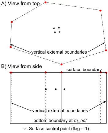
Those points that are required to define mesh geometry, including surface topography, electrode locations, internal boundaries (e.g., non-point electrodes, buried infrastructure, known geologic contacts), and mesh refinement points are specified as control points within the control points block. Each control point will become a mesh node in the final tetrahedral mesh. There are three types of control points: 1. Surface points are used to specify points of known elevation and/or surface electrode locations on the

mesh, and are given a flag of 1. E4D, triangle, and tetgen use these points to define surface topography and add nodes at surface electrode locations. Surface points cannot be placed on or beyond the outer boundary of the mesh (see Figure 5.1), which is specified by a set of surface boundary points, as described below.

2. Surface boundary points are used to define the outer boundary of the computational mesh, and are given a flag of 2 (see Figure 5.1). E4D uses these nodes to construct the outer vertical boundaries of the computational mesh by connecting adjacent points and constructing a series of vertical planes down to the elevation m_bot, which is specified in the general block.

3. Internal control points are used to define internal boundaries, buried electrode locations, and mesh refinement points, and are given a flag of 0 unless they are used to define a metallic boundary. Internal control points that are used to define a metallic boundary are assigned a negative integer, with each unique metallic boundary (point, line, plane, or volume) having a unique negative flag. All internal control points must be placed within the mesh boundaries formed by the surface boundary, vertical external boundaries, and bottom boundary (Figure 5.1).

Figure 5.1. Diagram of the three types of control points used to define a mesh

It is best practice to place a control point at every electrode location, although it is not explicitly required by E4D. E4D 'snaps' each electrode to the nearest node in the mesh. If the nearest node is far from the actual electrode location, modeling errors may result (E4D will print a warning message in modes 2 and higher if this occurs).

The format of the control point block is as follows:

Variable Type Description

n_cpts positive integer specifies the total number of control points

cp_num x y z b_flag see description

cp_num is a positive integer value that gives the index of the control points specified on this line. The cp_num values should be numbered consecutively from 1 to n_cpts. cp_num can be used to identify a particular control point used in a boundary definition as described in the internal boundary control block below.

x y and z are real valued numbers that give the easting, northing and elevation positions of control point cp_num respectively. b_flag is an integer value that provides the boundary flag for the control point specified on this line as described above.

There will be n_cpts of these lines in the control points block,

It is generally beneficial to refine the mesh near electrodes in order to improve modeling accuracy. For buried electrodes, this can be done by placing a second control point near each electrode control point. By so doing, tetgen will refine around the two points, as is required, to maintain a high quality mesh. The mesh can be refined around surface electrodes in the same manner. Another approach to refine around surface electrodes is to place each just under the surface with a boundary flag of b_flag = 0. By doing so, tetgen will automatically refine around each surface electrode. This practice also facilitates high quality surface mesh generation by removing the requirement to have a node at every electrode location on the surface (i.e., the electrodes are placed just beneath the surface).

5.6.3

Internal Boundary Configuration Block

Internal boundaries consist of one or more user-defined internal planes (called piecewise linear complexes in the tetgen documentation) that separate one region of the mesh from another. Internal boundaries that close to form a 'watertight' structure form a zone within the mesh. Boundaries are specified by describing how selected control points are connected to form planes within the internal boundary configuration block as follows:

Variable Type Description

n_plc non-negative

integer

total number of user-defined piecewise linear complex's (i.e. planes)

np b_num see description

np is the number of control points used to define this plane (there will be one np value listed for each of the n_plc planes defined)

b_num is the user specified boundary number for this plane. This integer can be any value except 0, 1, or 2, which are reserved within E4D. Set b_num >2 unless this boundary is an infinite conductivity (i.e. metallic) boundary, in which case b_num should be set to the same negative integer as b_flag, where b_flag is the boundary flag specified for each of the np control points used to defined this plane, as listed on the next line. All boundaries sharing the same negative b_num value are modeled as infinite conductivity and electrically

connected structures within E4D.

This line is the beginning of a plane definition. There will be

Variable Type Description

p1 p2 ... p_np non-negative integer

p* is the *th control point defining this plane. This value

references the control point indexes specified in the control points block. Control points must be specified in order to define a plane such that no segment connecting two consecutive control points crosses any other segment connecting two consecutive control points (i.e list the control points either clockwise or counter-clockwise). E4D does not check this condition prior to executing tetgen, and tetgen will fail if this condition is violated. Also, each of the points specified must lie in the same plane according to numerical precision or tetgen will fail.

This line is the end of a plane definition. There will be n_plc of lines in the internal boundary configuration block.

5.6.3.1 Critical boundary definition rules

The most common source of error in mesh generation is the improper specification of internal boundaries. If tetgen fails and the source of the error is not obvious from the mesh.log file, make sure the boundary definitions in the boundary configuration block adhere to the following requirements.

1) Do not define planes on any external boundary (e.g., surface, bottom, or side boundaries). E4D will construct these automatically. It is appropriate and required to explicitly specify segments of subsurface planes that intersect the surface boundary within the boundary definition (see item 5 below).

2) Ensure that boundaries do not intersect, except along common segments. Such intersections will cause tetgen to fail, and E4D does not check for this condition.

3) All control points existing within a defined plane, or along any segment of of a defined plane, must be included in the definition of that plane.

4) Each of the control points used in a plane definition must lie upon the same plane. This is important if four or more points are used to define a plane.

5) There are several import considerations when constructing boundaries that intersect the surface.

 The segments of any plane that intersect the surface boundary must be explicitly specified in the plane definition. In other words, any plane segment that intersects the surface boundary must not be defined by the first and last points specified in the plane definition (i.e. the points defining segments on the surface must be listed sequentially in the plane definition).

 It is often useful to specify a series of planes that form a closed boundary (thereby forming a zone) whose upper margin is the surface of the mesh, which is automatically generated by E4D (see item 1 above). In this case E4D must correctly connect the segments of planes intersecting the surface such that those segments define the upper boundary of the zone. To do so, E4D takes the list of control points defining the segments that intersect the surface, and connects each point to the next nearest point. With this in

mind, it is important to define the planes that intersect the surface in such a manner that E4D correctly connects the surface segments. Attention to this issue is only required for boundaries whose surface segments form convex angles.

It is generally helpful and highly recommend to draw a picture with relevant control points labelled to ensure that boundary definitions do not violate these conditions.

5.6.4

Hole Configuration Block

Any zone defined within E4D can be turned into a hole or void in the mesh. To create a hole, tetgen begins at one point within the subject zone and successively removes all of the elements enclosed within the zone boundary. The hole configuration block specifies which zones should be hollowed to form a hole by specifying a point within the zone as follows:

Variable Type Description

n_holes non-negative integer specifies the number of holes in the mesh

hn xh yh zh see description

hn is the index for this hole.

xh yh and zh are real valued numbers indicating the

easting, northing, and elevation of any point within this hole

There are n_holes of these lines, one for each hole, and hn

should range from 1 to n_holes.

Three-dimensional metallic structures should be defined as holes in E4D, so that only the shell of the structure exists in the mesh. This is done by specifying a hole point inside of a zone constructed using planes with the same negative boundary flag as described above.

5.6.5

Zone Configuration Block

The zone configuration block assigns maximum element volumes, conductivity values, and zone numbers to each zone.

Variable Type Description

n_zones positive integer number of user-defined zones

zn xz yz zz mz_vol zcond see description

zn is the zone number assigned to this zone. xz yz zz is the position of any point within this zone mz_vol is the maximum volume of any point within this zone

zcond is the conductivity of this zone

There are n_zones of these lines, one for each zone in

the mesh. These lines should be listed

consecutivelyfrom zn = 1 to zn = n_zones.

Zones that are not configured will assume a maximum volume constraint of max_evol_def (see general block) and a default conductivity value. However, it is best practice to provide configuration options for each zone defined in the mesh.

5.6.6

Visualization Options Block

The visualization options block provides the option to automatically produce an exodus file for visualization once the mesh is generated as follows:

Variable Type Description

bx_flag integer value (0 or 1)

specifies whether E4D should build an exodus for mesh visualization (1) or not (0)

bx_loc string

specifies the location of the utility program bx. For example, if bx is located in /usr/e4d_qc/bin/, then bx_loc is '/usr/e4d_qc/bin/bx' (quotes are required). If /usr/e4d_qc/bin is in the executable path, then 'bx' will suffice.

mtr_opt integer (0 or 1)

mtr_opt is the mesh translation option. If mtr_opt is set to 1 then the mesh is translated internally to preserve numerical precision. If mtr_opt is set to 0, the mesh translation is not applied.

Mesh translation occurs internally to E4D, and does not affect user interface in general use (i.e. results are always reported in the original coordinates). Mesh translation is particularly important when using global coordinate systems, and is generally recommended.

5.7

ER Mesh Generation Tutorial 1.1: Two Buried Blocks

5.7.1

Conceptual Diagram

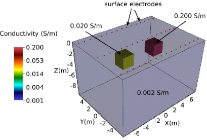
In this example, we build a mesh comprising surface electrodes, two subsurface boxes, a foreground zone defined for convenient visualization, and a boundary zone that extends from the foreground zone to the external boundaries. A conceptual diagram of the mesh, including control points and zone

assignments to be defined in the mesh configuration file, is shown in Figure 5.2. The mesh consists of three lines of surface electrodes, where line 1 includes control points 1 through 16, line 2 includes control

points 17 through 32, and line 3 includes control points 33 through 48. Control points 49 through 52 and 57 through 60 define the foreground region, which is assigned to be zone 1. Control points 61 through 68 define the western-most box, which is assigned to be zone 2. Control points 69 through 76 define the eastern-most box, which is assigned to be zone 3. The region extending from the foreground to the outer boundaries is not shown, but is assigned to be zone 4. The mesh configuration file for Figure 5.2 (two_blocks.cfg) is shown below with annotations denoting the corresponding mesh configuration file variables described above. It is also included with the E4D distribution

under <e4d_dir>tutorial/mode_1/two_blocks/two_blocks.cfg.

Figure 5.2. Control point and zone map for mesh configuration file two_blocks.cfg. External boundary points 54-56 and internal refine points 77-124 are not shown. The part of the domain extending from zone 1 to the external boundaries (zone 4) is also not shown.

5.7.2

Building the Mesh

In addition to the mesh configuration file, the run configuration file e4d.inp is needed to build the mesh. In mode 1, the only file that must be listed is the mesh configuration file. The run configuration file for this example is shown below.

<begin run configuration file e4d.inp> (this line is not included in the file) 1

two_blocks.cfg

To build the mesh, execute the command:

<e4d_dir>/bin/mpirun -np 1 <e4d_dir>/bin/e4d

or

mpirun -np 1 e4d

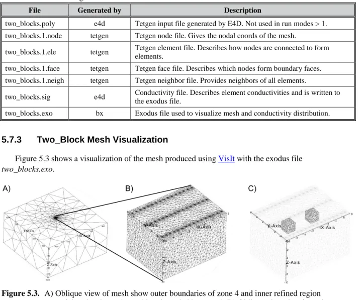
if <e4d_dir>/binis in the executable path, where <e4d_dir> is the E4D installation directory. E4D builds the input files for triangle and tetgen, and calls each to build the mesh. E4D then builds a conductivity file for the mesh as specified in the mesh configuration file, and calls bx to build an exodus file for

visualization. The files generated include:

File Generated by Description

two_blocks.poly e4d Tetgen input file generated by E4D. Not used in run modes > 1. two_blocks.1.node tetgen Tetgen node file. Gives the nodal coords of the mesh.

two_blocks.1.ele tetgen Tetgen element file. Describes how nodes are connected to form elements.

two_blocks.1.face tetgen Tetgen face file. Describes which nodes form boundary faces. two_blocks.1.neigh tetgen Tetgen neighbor file. Provides neighbors of all elements.

two_blocks.sig e4d Conductivity file. Describes element conductivities and is written to the exodus file.

two_blocks.exo bx Exodus file used to visualize mesh and conductivity distribution.

5.7.3

Two_Block Mesh Visualization

Figure 5.3 shows a visualization of the mesh produced using VisIt with the exodus file

two_blocks.exo.

Figure 5.3. A) Oblique view of mesh show outer boundaries of zone 4 and inner refined region comprising the electrodes and box bounded by zone 1. B) Oblique view showing other boundaries of zone 1 and mesh refinement at electrode locations. C) Oblique view with zone 1 boundaries shown in transparency to reveal zone 2 and zone 3 boundaries.

<begin file two_blocks.cfg> this line is not included in two_blocks.cfg 1.3 1e12 mesh quality (m_qual) max volume (max_evol_def) -500 bottom of mesh elevation (m_bot)

1 flag to build mesh (tet_build_flag) "tetgen" command to run tetgen (tet_loc) "triangle" command to run triangle (tri_loc) 124 number of control points (n_cpts) 1 -7.5 -5 0 1 1 x1 y1 z1 b_flag_1 2 -6.5 -5 0 1 2 x2 y2 z2 b_flag_2 3 -5.5 -5 0 1 . 4 -4.5 -5 0 1 . 5 -3.5 -5 0 1 . 6 -2.5 -5 0 1 7 -1.5 -5 0 1 8 -0.5 -5 0 1 9 0.5 -5 0 1 10 1.5 -5 0 1 11 2.5 -5 0 1 12 3.5 -5 0 1 13 4.5 -5 0 1 14 5.5 -5 0 1 15 6.5 -5 0 1 16 7.5 -5 0 1 17 -7.5 0 0 1 18 -6.5 0 0 1 19 -5.5 0 0 1 20 -4.5 0 0 1 21 -3.5 0 0 1 22 -2.5 0 0 1 23 -1.5 0 0 1 24 -0.5 0 0 1 25 0.5 0 0 1 26 1.5 0 0 1 27 2.5 0 0 1 28 3.5 0 0 1 29 4.5 0 0 1 30 5.5 0 0 1 31 6.5 0 0 1 32 7.5 0 0 1 33 -7.5 5 0 1 34 -6.5 5 0 1 35 -5.5 5 0 1 36 -4.5 5 0 1 37 -3.5 5 0 1 38 -2.5 5 0 1 39 -1.5 5 0 1 40 -0.5 5 0 1 41 0.5 5 0 1 42 1.5 5 0 1 43 2.5 5 0 1 44 3.5 5 0 1 45 4.5 5 0 1 46 5.5 5 0 1 47 6.5 5 0 1 48 7.5 5 0 1

49 -8 -6 0 1 upper control points for foreground (zone 1) 50 -8 6 0 1

51 8 6 0 1 52 8 -6 0 1

53 -500 -500 0 2 boundary control points 54 -500 500 0 2

55 500 500 0 2 56 500 -500 0 2

57 -8 -6 -10 0 lower control points for forground (zone 1) 58 -8 6 -10 0

59 8 6 -10 0 60 8 -6 -10 0

61 -4.0 -1.0 -1.0 0 Upper control points for left block (zone 2) 62 -4.0 1.0 -1.0 0

63 -2.0 1.0 -1.0 0 64 -2.0 -1.0 -1.0 0

65 -4.0 -1.0 -3.0 0 lower control points for left block (zone 2) 66 -4.0 1.0 -3.0 0

67 -2.0 1.0 -3.0 0 68 -2.0 -1.0 -3.0 0

69 4.0 -1.0 -1.0 0 upper control points for right block (zone 3) 70 4.0 1.0 -1.0 0

71 2.0 1.0 -1.0 0 72 2.0 -1.0 -1.0 0

73 4.0 -1.0 -3.0 0 lower control points for right block (zone 3) 74 4.0 1.0 -3.0 0

75 2.0 1.0 -3.0 0 76 2.0 -1.0 -3.0 0

77 -7.5 -5 -0.05 0 additional points for electrode refinement 78 -6.5 -5 -0.05 0 79 -5.5 -5 -0.05 0 80 -4.5 -5 -0.05 0 81 -3.5 -5 -0.05 0 82 -2.5 -5 -0.05 0 83 -1.5 -5 -0.05 0 84 -0.5 -5 -0.05 0 85 0.5 -5 -0.05 0 86 1.5 -5 -0.05 0 87 2.5 -5 -0.05 0 88 3.5 -5 -0.05 0 89 4.5 -5 -0.05 0 90 5.5 -5 -0.05 0 91 6.5 -5 -0.05 0 92 7.5 -5 -0.05 0 93 -7.5 0 -0.05 0 94 -6.5 0 -0.05 0 95 -5.5 0 -0.05 0 96 -4.5 0 -0.05 0

97 -3.5 0 -0.05 0 98 -2.5 0 -0.05 0 99 -1.5 0 -0.05 0 100 -0.5 0 -0.05 0 101 0.5 0 -0.05 0 102 1.5 0 -0.05 0 103 2.5 0 -0.05 0 104 3.5 0 -0.05 0 105 4.5 0 -0.05 0 106 5.5 0 -0.05 0 107 6.5 0 -0.05 0 108 7.5 0 -0.05 0 109 -7.5 5 -0.05 0 110 -6.5 5 -0.05 0 111 -5.5 5 -0.05 0 112 -4.5 5 -0.05 0 113 -3.5 5 -0.05 0 114 -2.5 5 -0.05 0 115 -1.5 5 -0.05 0 116 -0.5 5 -0.05 0 117 0.5 5 -0.05 0 118 1.5 5 -0.05 0 119 2.5 5 -0.05 0 120 3.5 5 -0.05 0 121 4.5 5 -0.05 0 122 5.5 5 -0.05 0 123 6.5 5 -0.05 0 124 7.5 5 -0.05 0

17 number of internal planes (n_plc)

4 10 number of points in plc 1 (np1), boundary number(b_num_1) 49 50 58 57 control points in plc 1: western boundary of zone 1

4 10 np2 b_num_2

50 51 59 58 control points in plc 2: northern boundary of zone 1 4 10

51 52 60 59 eastern boundary of zone 1 4 10

52 49 57 60 southern boundary of zone 1 4 10

57 58 59 60 bottom boundary of zone 1 4 11

61 62 66 65 western boundary of zone 2 4 11

62 63 67 66 northern boundary of zone 2 4 11

63 64 68 67 eastern boundary of zone 2 4 11

64 61 65 68 southern boundary of zone 2 4 11

61 62 63 64 upper boundary of zone 2 4 11

65 66 67 68 lower boundary of zone 2 4 12

69 70 74 73 eastern boundary of zone 2 4 12

4 12

71 72 76 75 western boundary of zone 2 4 12

72 69 73 76 southern boundary of zone 2 4 12

69 70 71 72 upper boundary of zone 2 4 12

73 74 75 76 lower boundary of zone 2

0 number of holes(n_holes) 4 number of zones(n_zones)

1 0.0 0.0 -5.0 0.1 0.002 zone1 xz_1 yz_1 zz_1 mz_vol_1 cond_1 2 -2.5 0.0 -2.5 0.01 0.002 zone2 xz_2 yz_2 zz_2 mz_vol_2 cond_2 3 2.5 0.0 -2.5 0.01 0.002 .

4 0.0 0.0 -20.0 1e12 0.002 .

1 flag to build exodus file (bex_flag) 'bx' command to build exodus file (bex_loc)

1 translate the mesh internally to preserve numerical precision

<end file two_blocks.cfg> this line is not included in two_blocks.cfg

5.8

ER Mesh Generation Tutorial 1.2: Buried Metallic Box, Sheet,

and Line

5.8.1

Overview

In this example, we demonstrate how to build a mesh with infinite conductivity inclusions. This example builds upon concepts presented in ER Mesh Generation Tutorial 1.1; users are encouraged to review and understand that example prior to reviewing this example.

5.8.2

Conceptual Diagram

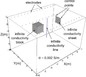
In this example, we build a mesh comprising surface electrodes, three buried infinite conductivity structures (a box, a sheet, and a line), a foreground zone defined for convenient visualization, and a boundary zone that extends from the foreground zone to the external boundaries. A conceptual diagram of the subsurface is shown in Figure 5.4. The mesh consists of three lines of surface electrodes, where line 1 includes control points 1 through 16, line 2 includes control points 17 through 32, and line 3 includes control points 33 through 48. Control points 49 through 52 and 57 through 60 define the foreground region, which is assigned zone 1. Control points 61 through 68 define the conductive box. Control points 69,70,73 and 74 through 76 define the conductive sheet, and points 125-148 define the conductive line. The region extending from the foreground to the outer boundaries is not shown, but is assigned zone 2. The mesh configuration file for Figure 5.4 (mbsl.cfg) is shown below, with annotations denoting the corresponding mesh configuration file variables described in the mesh generation section of the user guide. It is also included with the E4D distribution under

Figure 5.4. Conceptual diagram of surface electrodes with a subsurface containing an infinite

conductivity box, sheet, and line embedded in a background medium with a conductivity of 0.002 S/m. Each of the control points and electrode points shown are listed in the mesh configuration file mbsl.cfg.

5.8.3

Building the mbsl Mesh

In addition to the mesh configuration file, the run configuration file e4d.inp is needed to build the mesh. In mode 1, the only file that must be listed is the mesh configuration file. The run configuration file for this example is shown below.

<begin run configuration file e4d.inp> (this line is not included in the file) 1

mbsl.cfg

<end run configuration file e4d.inp> (this line is not included in the file)

To build the mesh, execute the command:

<e4d_dir>/bin/mpirun -np 1 <e4d_dir>/bin/e4d

or

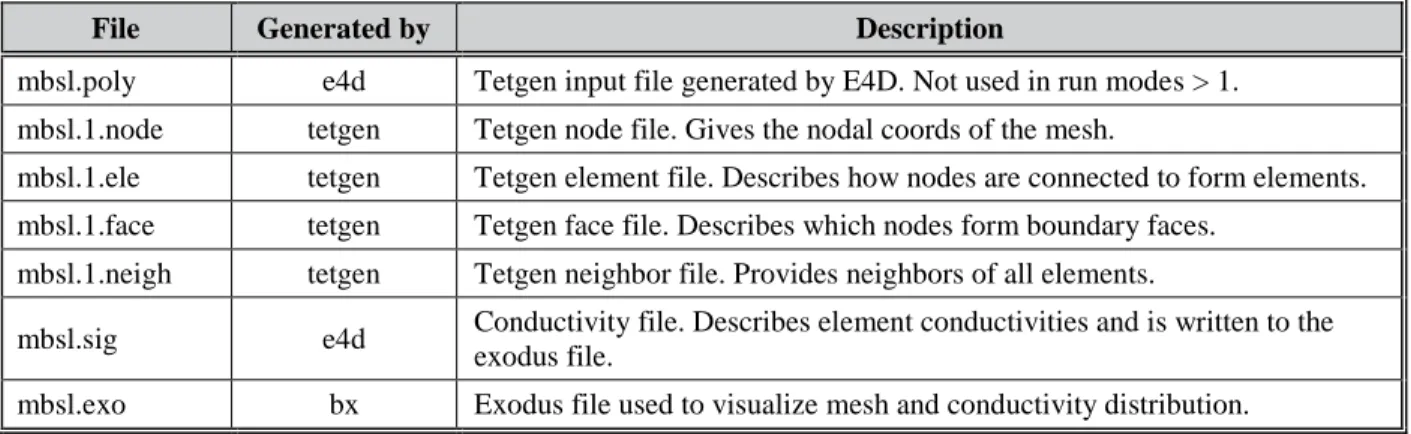
if <e4d_dir>/binis in the executable path, where <e4d_dir> is the E4D installation directory. E4D builds the input files for triangle and tetgen, and calls each to build the mesh. E4D then builds a conductivity file for the mesh as specified in the mesh configuration file, and calls bx to build an exodus file for

visualization. The files generated include:

File Generated by Description

mbsl.poly e4d Tetgen input file generated by E4D. Not used in run modes > 1. mbsl.1.node tetgen Tetgen node file. Gives the nodal coords of the mesh.

mbsl.1.ele tetgen Tetgen element file. Describes how nodes are connected to form elements. mbsl.1.face tetgen Tetgen face file. Describes which nodes form boundary faces.

mbsl.1.neigh tetgen Tetgen neighbor file. Provides neighbors of all elements.

mbsl.sig e4d Conductivity file. Describes element conductivities and is written to the exodus file.

mbsl.exo bx Exodus file used to visualize mesh and conductivity distribution.

5.8.4

mbsl Mesh Visualization

Figure 5.5 shows a visualization of the mesh produced using VisIt with the exodus file mbsl.exo.

Figure 5.5. Cut-out view of the mbsl mesh showing nodes added by tetgen for the three infinite

conductivity boundaries. Note that the grey region representing the infinite conductivity box is shown only for reference. The mesh is hollow in the interior of the box; only the outer boundary of the box is included in the mesh.

5.8.5

Mesh Configuration File:

mbsl.cfg

<begin mesh configuration file mbsl.cfg> this line is not included in two_blocks.cfg

1.3 1e12 mesh quality (m_qual), max volume (max_evol_def) -500 bottom of mesh elevation (m_bot)

1 flag to build mesh (tet_build_flag) "tetgen" command to run tetgen (tet_loc) "triangle" command to run triangle (tri_loc) 148 number of control points (n_cpts) 1 -7.5 -5 0 1 1 x1 y1 z1 b_flag_1 2 -6.5 -5 0 1 2 x2 y2 z2 b_flag_2 3 -5.5 -5 0 1 . 4 -4.5 -5 0 1 . 5 -3.5 -5 0 1 . 6 -2.5 -5 0 1 7 -1.5 -5 0 1 8 -0.5 -5 0 1 9 0.5 -5 0 1 10 1.5 -5 0 1 11 2.5 -5 0 1 12 3.5 -5 0 1 13 4.5 -5 0 1 14 5.5 -5 0 1 15 6.5 -5 0 1 16 7.5 -5 0 1 17 -7.5 0 0 1 18 -6.5 0 0 1 19 -5.5 0 0 1 20 -4.5 0 0 1 21 -3.5 0 0 1 22 -2.5 0 0 1 23 -1.5 0 0 1 24 -0.5 0 0 1 25 0.5 0 0 1 26 1.5 0 0 1 27 2.5 0 0 1 28 3.5 0 0 1 29 4.5 0 0 1 30 5.5 0 0 1 31 6.5 0 0 1 32 7.5 0 0 1 33 -7.5 5 0 1 34 -6.5 5 0 1 35 -5.5 5 0 1 36 -4.5 5 0 1 37 -3.5 5 0 1 38 -2.5 5 0 1 39 -1.5 5 0 1 40 -0.5 5 0 1 41 0.5 5 0 1 42 1.5 5 0 1 43 2.5 5 0 1

44 3.5 5 0 1 45 4.5 5 0 1 46 5.5 5 0 1 47 6.5 5 0 1 48 7.5 5 0 1

49 -8 -6 0 1 upper control points for foreground (zone 1) 50 -8 6 0 1

51 8 6 0 1 52 8 -6 0 1

53 -500 -500 0 2 boundary control points 54 -500 500 0 2

55 500 500 0 2 56 500 -500 0 2

57 -8 -6 -10 0 lower control points for forground (zone 1) 58 -8 6 -10 0

59 8 6 -10 0 60 8 -6 -10 0

61 -4.0 -1.0 -1.0 -1 Upper control points conductive block 62 -4.0 1.0 -1.0 -1

63 -2.0 1.0 -1.0 -1 64 -2.0 -1.0 -1.0 -1

65 -4.0 -1.0 -3.0 -1 lower control points conductive block 66 -4.0 1.0 -3.0 -1

67 -2.0 1.0 -3.0 -1 68 -2.0 -1.0 -3.0 -1

69 4.0 -1.0 -1.0 -2 control points 69-70 define the upper edge of the metal sheet 70 4.0 1.0 -1.0 -2

71 2.0 1.0 -1.0 0 72 2.0 -1.0 -1.0 0

73 4.0 -1.0 -3.0 -2 control points 73-74 define the lower edge of the metal sheet 74 4.0 1.0 -3.0 -2

75 2.0 1.0 -3.0 0 76 2.0 -1.0 -3.0 0

77 -7.5 -5 -0.05 0 additional points for electrode refinement 78 -6.5 -5 -0.05 0 79 -5.5 -5 -0.05 0 80 -4.5 -5 -0.05 0 81 -3.5 -5 -0.05 0 82 -2.5 -5 -0.05 0 83 -1.5 -5 -0.05 0 84 -0.5 -5 -0.05 0 85 0.5 -5 -0.05 0 86 1.5 -5 -0.05 0 87 2.5 -5 -0.05 0 88 3.5 -5 -0.05 0 89 4.5 -5 -0.05 0 90 5.5 -5 -0.05 0 91 6.5 -5 -0.05 0

92 7.5 -5 -0.05 0 93 -7.5 0 -0.05 0 94 -6.5 0 -0.05 0 95 -5.5 0 -0.05 0 96 -4.5 0 -0.05 0 97 -3.5 0 -0.05 0 98 -2.5 0 -0.05 0 99 -1.5 0 -0.05 0 100 -0.5 0 -0.05 0 101 0.5 0 -0.05 0 102 1.5 0 -0.05 0 103 2.5 0 -0.05 0 104 3.5 0 -0.05 0 105 4.5 0 -0.05 0 106 5.5 0 -0.05 0 107 6.5 0 -0.05 0 108 7.5 0 -0.05 0 109 -7.5 5 -0.05 0 110 -6.5 5 -0.05 0 111 -5.5 5 -0.05 0 112 -4.5 5 -0.05 0 113 -3.5 5 -0.05 0 114 -2.5 5 -0.05 0 115 -1.5 5 -0.05 0 116 -0.5 5 -0.05 0 117 0.5 5 -0.05 0 118 1.5 5 -0.05 0 119 2.5 5 -0.05 0 120 3.5 5 -0.05 0 121 4.5 5 -0.05 0 122 5.5 5 -0.05 0 123 6.5 5 -0.05 0 124 7.5 5 -0.05 0

125 0 0 -0.25 -3 points 125 - 126 define a metallic line (e.g. well casing) 126 0 0 -0.5 -3 127 0 0 -0.75 -3 128 0 0 -1 -3 129 0 0 -1.25 -3 130 0 0 -1.5 -3 131 0 0 -1.75 -3 132 0 0 -2 -3 133 0 0 -2.25 -3 134 0 0 -2.5 -3 135 0 0 -2.75 -3 136 0 0 -3 -3 137 0 0 -3.25 -3 138 0 0 -3.5 -3 139 0 0 -3.75 -3 140 0 0 -4 -3 141 0 0 -4.25 -3 142 0 0 -4.5 -3 143 0 0 -4.75 -3 144 0 0 -5 -3 145 0 0 -5.25 -3 146 0 0 -5.5 -3

147 0 0 -5.75 -3 148 0 0 -6 -3

12 number of internal planes (n_plc)

4 10 number of points in plc 1 (np1), boundary number(b_num_1) 49 50 58 57 control points in plc 1: western boundary of zone 1

4 10 np2 b_num_2

50 51 59 58 control points in plc 2: northern boundary of zone 1 4 10 .

51 52 60 59 eastern boundary of zone 1 4 10 .

52 49 57 60 southern boundary of zone 1 4 10 .

57 58 59 60 bottom boundary of zone 1 4 -1

61 62 66 65 western boundary of metal box 4 -1

62 63 67 66 northern boundary of metal box 4 -1

63 64 68 67 eastern boundary of metal box 4 -1

64 61 65 68 southern boundary of metal box 4 -1

61 62 63 64 upper boundary of metal box 4 -1

65 66 67 68 lower boundary of metal box 4 -2

69 70 74 73 metal sheet

1 number of holes ... 1 for the metal box 2 -2.5 0.0 -2.5 point inside the metal box

2 number of zones ... 2

1 0.0 0.0 -5.0 0.1 0.002 1 xz_1 yz_1 zz_1 mz_vol_1 cond_1 2 0.0 0.0 -20.0 1e12 0.002

1 flag to build exodus file (bex_flag) '../../../bin/bx' command to build exodus file (bex_loc)

1 translate the mesh internally to preserve numeric precision

6.0

Mode 2: ER Forward Run Mode

6.1

Introduction

Forward modeling is defined herein as the process whereby E4D simulates and reports the subsurface electrical potential generated (real and/or complex) per ampere of transmitted current, given the

subsurface conductivity distribution specified in the conductivity file listed in e4d.inp. Results are reported as simulated measurements and/or simulated potential distributions according to specifications givenin the output options file listed in e4d.inp. The general flow for forward modeling is shown below.

1. Generate the computational mesh

The first step in forward modeling is generating the computational mesh. Mesh generation is described in the previous chapter. The basic steps for generating the mesh include constructing the mesh configuration file, executing the mesh generation with E4D, and visualizing the results using bx and VisIt. A conductivity file is automatically generated as part of the mesh generation process, where the conductivity value is specified for each zone defined in the mesh. It is also possible to construct user-defined conductivity files outside of E4D (e.g., using stochastic simulation software) for forward modeling. Examples are provided in Sections 7.9.4 and 9.1.2.

2. Generate the survey file

Survey files give the locations of electrodes, define how those electrodes are used to generate a survey, and specify observed measurements and standard deviations. In forward modes, measurement results and standard deviations are not used, but placeholders must be included in the survey file. 3. Generate the output options file

The output options file specifies how simulated results should be reported, including simulated measurements and/or specified subsurface potential distributions for visualization. If specified in the output options file, simulated survey results are written to the simulated data file, and potential distributions are written to potential files.

4. Once the mesh has been generated, and the survey file and output option files have been constructed,

the e4d.inpfile is constructed and E4D is executed using the command:

mpirun -np <num_proc> e4d

where num_procis the number of processors E4D should use during execution, which must be at least 2 and no more than ne+1 where ne is the number of electrodes plus the number of infinite conductivity (i.e., metallic) inclusions in the simulation.

5. Upon successful forward execution, E4D generates a number of output files as specified in the output options file. If potential distributions are generated, they may be investigated using bx to build a