The Valuation of Natural Gas Storage: A Knowledge Gradient Approach with. Non-Parametric Estimation

(1)

The Valuation of Natural Gas Storage:

A Knowledge Gradient Approach with

Non-Parametric Estimation

By: Jennifer Schoppe

Advisor: Professor Warren B. Powell

Submitted in partial fulfillment

Of the requirements for the degree of

Bachelor of Science in Engineering

Department of Operations Research and Financial Engineering

Princeton University

(2)

ii

I hereby declare that I am the sole author of this thesis.

I authorize Princeton University to lend this thesis to other institutions or individuals for the purpose of scholarly research.

________________________________________ Jennifer Schoppe

I further authorize Princeton University to reproduce this thesis by photocopying or by other means, in total or in part, at the request of other institutions or individuals for the purpose of scholarly research.

________________________________________ Jennifer Schoppe

(3)

iii

Dedication

To my unforgettable Princeton experience,

my parents who gave me the opportunity to take the journey, and my sister who was with me through every moment.

(4)

iv

Acknowledgements

There are many people who helped bring this thesis into existence, and I would like to extend my gratitude though the thanks they deserve extends beyond what can be expressed on this page.

Within the ORFE Department, I would first like to thank my advisor Professor Warren Powell for his enthusiasm, insight, and encouragement to make my thesis better. My gratitude extends to Dr. Hugo Simao for his computational expertise and Michael Coulon for his knowledge on energy pricing processes. A special thanks goes to Emre Barut, for allowing this thesis the opportunity to be one of the first to test his research in non-parametric estimators for knowledge gradient methods. His time and energy spent in providing both computational and theoretical support is greatly appreciated.

I would like to thank James Schoppe at Iberdrola Renewables and Richard Adamczyk at Enstor Operating Company for providing me with invaluable resources regarding the natural gas industry and storage.

I would like to acknowledge Doug Eshleman and Mike Hasling for their time and patience in answering my questions as I navigated through the world of computer programming.

I would also like to thank Stephanie Schoppe for copyediting this work. I have been blessed to have many people in my life who have offered me love and encouragement through all my achievements including the creation of this thesis. They are my parents, my grandparents, my sister, and my friends. Many thanks to all.

(5)

v

Abstract

This thesis examines the problem of natural gas storage valuation focusing on the valuation of high-deliverability gas storage facilities, specifically salt cavern storage. We present capable valuation analysis and optimization methodologies that accurately account for the various operating characteristics of real storage facilities as well as the complex stochastic nature of natural gas prices. We use an extension of the Knowledge Gradient Algorithm, a sequential learning method, which incorporates non-parametric estimation in order to present a method that produces a quality valuation with minimal computational burden. The results of the method will present an optimal strategy for the operation of the natural gas storage facility, as well as yield a value for the facility.

(6)

vi

Table of Figures

Figure 1- Natural Gas Powered Generation Plant ... 2

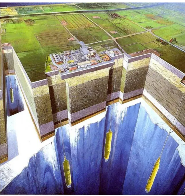
Figure 2 - Salt Cavern Facilities ... 3

Figure 3 - Preparing Hole for the Explosive Charges Used in Seismic Exploration ... 5

Figure 4 - Shale Deposits ... 6

Figure 5 - Alaskan Pipeline Carrying Natural Gas ... 7

Figure 6 - Natural Gas from Wellhead to End-Users ... 8

Figure 7 - Henry Hub in Erath, Louisiana ... 10

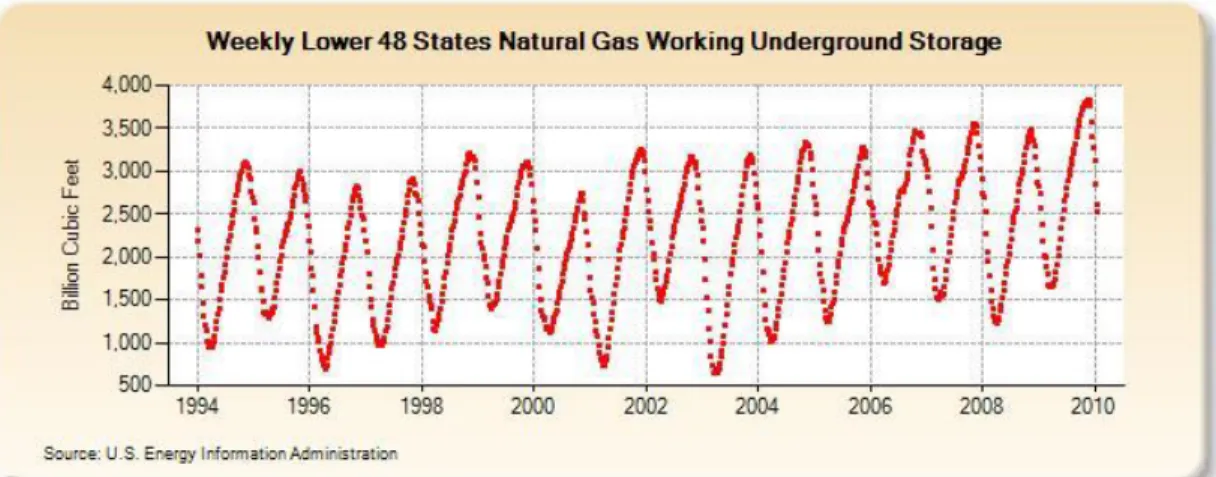
Figure 8 - Fluctuations in Underground Storage Volume ... 12

Figure 9 - Breakdown of Storage Portfolio in United States ... 15

Figure 10 - Depleted Reservoir ... 16

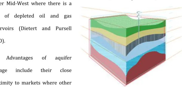
Figure 11- Aquifer Storage ... 17

Figure 12 - Salt Cavern... 18

Figure 13 - Illustration of Knowledge Gradient ... 34

Figure 14 – Knowledge Gradient with Correlated Beliefs at Measurements 1... 37

Figure 15- Knowledge Gradient with Correlated Beliefs at Measurement 5 ... 37

Figure 16 - Knowledge Gradient with Correlated Beliefs Estimated Surface ... 38

Figure 17 - Plot of Kernel Functions K(u) ... 40

Figure 18 - Henry Hub Historical Natural Gas Spot Prices 2004 - 2009 ... 48

Figure 19 - Natural Gas Spot Prices with Exponential Smoothing, Beta = .002 ... 50

Figure 20 - Sample Paths for 1-Year of Simulated Natural Gas Spot Prices ... 52

Figure 21 - Simulated Month Ahead Forward Prices for One Year ... 54

Figure 22 - Month Ahead Forward Prices with Spot Prices for One Month ... 55

Figure 23 – Swing Trend with 10% Filtering ... 68

Figure 24 - Swing Trend with 5% Filtering ... 68

Figure 25 - Policy 0: Second Measurement ... 77

Figure 26 - Policy 0: 25 Measurements ... 79

Figure 27- Policy 0: 100 Measurements ... 79

(10)

x

Figure 32 - Withdrawal Rate's Effect on Storage Value ... 87

Figure 33- Policy 0, KGNP Result for Doubled Volatility ... 88

Figure 34 - Policy 0: S-Curve ... 89

Figure 35 - Policy 1: S-Curve ... 90

(11)

CHAPTER 1 Introduction

In late November 2009, the burgeoning glut of the U.S. natural gas supply ventured into uncharted terrain as the Energy Information Administration (EIA) reported the volume of working gas within U.S. storage to have hit 3.837 trillion cubic feet (Tcf). This expansion is mirrored in the demand for natural gas, which has called more and more supply away from its historical use in residential and industry sectors to the power generation sector. Natural gas is playing an increasing role in power generation, and in 2009, 23,475 MW of new generation capacity was planned in the U.S. with over 50% being natural gas fired additions (Energy Information Administration 2004). Figure 1 shows one of the many rapidly emerging gas powered generation plants.

The natural gas market is rapidly changing, and natural gas storage will play a significant role as it buffers demand and regulates supply. However, with shifting supply and demand, other functions of storage can be utilized such as with salt caverns, which exhibit high deliverability, high injection and withdrawal capacity,

(12)

CHAPTER 1: Introduction

2

that can quickly respond to changing gas prices; and thus are utilized as an arbitrage mechanism. Storage owners and service providers will need to reexamine the value of their facilities which is derived

from the expected profit from the operations of a facility.

The problem of the valuation of a natural gas storage facility is not new, and literature has been produced within the industry as well

as in academic circles. Industry professionals employ linear optimization with Monte Carlo methods (Byers 2006) while the academic community supports the use of stochastic optimization with an Approximate Dynamic Programming approach (Lai, Margot and Secomandi 2008). Unfortunately, there remains advantages and disadvantage of both techniques rendering it ambiguous to decipher the superior procedure.

We will examine the problem of natural gas storage valuation focusing on the valuation of high-deliverability gas storage facilities, specifically salt cavern storage as pictured in Figure 2. We will strive to present capable valuation analysis and optimization methodologies that accurately account for the various operating characteristics of real storage facilities as well as the complex stochastic nature of natural gas prices.

(13)

3

Figure 2 - Salt Cavern Facilities (Energy Information Administration 2004)

To solve the problem we will utilize stochastic optimization methods within the realm of Optimal Learning. The idea encompasses a stochastic search over policies which dictate the operational decisions of the storage facility. We assume the policies are composed of a set of tunable parameters, and through sequential measurements of the alternatives, estimates of each policy’s performance can be ascertained. The goal is to choose the alternatives, and subsequently the policy,

(14)

4

which will produce the best performance. A strong performer within sequential learning algorithms is the knowledge gradient which was developed by Gupta & Miescke (1996) and later analyzed by Frazier et al. (2008). This algorithm strives to maximize the amount of knowledge obtained with each measurement in an effort to obtain an improved solution with the new knowledge. We will use an innovative method newly added to the literature on the knowledge gradient algorithm that evaluate problems with correlated beliefs using non-parametric estimation (Barut and Powell 2010). The results of the method will account for an optimal strategy for the operation of the natural gas storage facility, as well as yield a value for the facility.

1.1 Natural Gas: From Wellhead to Market

Though it may be simple to flip on one’s burner in the kitchen, the process of getting natural gas from the ground and into everyday life is actually an extensive and complex process. This section provides an overview of the process, journeying from exploration to marketing of the natural gas that will be sold for homes and industry.

1.1.1 Exploration and Extraction

The process begins with geologists and geophysicists, who use technology and knowledge of the properties of underground natural gas deposits to gather data and make educated guesses as to where natural gas deposits may exist thousands of feet below ground. The most important tool in exploration is the use of basic seismology which refers to the study of how energy moves through the Earth's crust

(15)

5

and interacts differently with various types of underground formations. The energy can be mapped, providing an effective way to image both sources and structures deep within the Earth. In both onshore and offshore exploration, seismic waves are created that can travel through the Earth's crust and generate the reflections needed to ascertain the presence of natural gas or the properties of a reservoir formation (NaturalGas.org 2004). Figure 3 shows operators preparing a hole for the explosive charges used in seismic exploration.

After extensive measurements deem that the site may be enriched with a marketable quantity of natural gas, drilling can begin. However, the exploration team may be incorrect in its estimation of the existence of natural gas at a well site. If this occurs, the well is labeled a 'dry well,' and production does not proceed. Conversely, if the new well is drilled and comes in contact with natural gas deposits, it is developed to allow the extraction of the natural gas and is labeled as a 'productive' well (NaturalGas.org 2004).

A common misconception is that all natural gas is extracted from natural gas wells. In fact, natural gas is extracted from a variety of sources oil wells, shale, and coalbeds. Oil wells which contain natural gas are known as “associated” wells. Even

Figure 3 - Preparing Hole for the Explosive Charges Used in Seismic Exploration (Energy Information Administration 2004)

(16)

6

if the well is specifically drilled for oil extraction, natural gas will almost always be a byproduct of producing oil, since the small, light gas carbon chains come out of solution as it undergoes pressure reduction from the reservoir to the surface. An unconventional source of natural gas is shale, a fine-grained sedimentary rock which can contain natural gas within its

layered formation pictured in Figure 4. In recent years, shale deposits have accounted for an increasing share of the natural gas production. As of November 2008, FERC estimated that there are 742 Tcf of recoverable shale gas in the United States. A second unconventional source is

coalbed methane. Coal deposits are commonly found as seams that run underground. Many coal seams also contain natural gas, either within the seam itself or the surrounding rock which can be extracted and transported for production (NaturalGas.org 2004). Table 1 lists the sources of natural gas and the amount of natural gas extracted from each in the year 2008.

Table 1 - Sources of Natural Gas and Production Volume (Energy Information Administration 2004)

Type of Well Gross Production for 2008 % of Total Production Natural Gas Well 18,011,151 MMcf 64.84%

Oil Well 5,844,798 MMcf 21.05% Shale Deposits 2,022,000 MMcf 7.28%

Coalbed 1,898,400 MMcf 6.83%

(17)

7 1.1.2 Production and Transport

Although consisting of mostly methane, the gas extracted at the wellhead is considered “raw” and can be mixed with oil or other hydrocarbons such as ethane, propane, butanes, and pentanes. In order to maintain pipeline quality, regulations are in place to ensure only purified natural gas is transported. Typically, some of the needed processing is accomplished at the well site and later completed at processing plants connected through gathering pipelines. Some of the hydrocarbons associated with the natural gas are very valuable and are known as natural gas liquids (NGL). NGLs have a

variety of uses and can be sold separately from the natural gas (NaturalGas.org 2004).

Once the natural gas has been purified, it enters

into a complex network of pipelines that make up the transportation system for natural gas. The system is designed to quickly and efficiently transport natural gas from the plant, to areas of high natural gas demand for use. It is composed of interstate and intrastate pipelines which are responsible for transporting natural gas at high speeds and pressure throughout the country and within a particular state respectively. Natural gas will usually travel great distances before reaching the end user. Figure 5 shows the Alaskan pipeline which carries natural gas over 800 miles.

(18)

8 1.1.3 Storage

Should natural gas not be required at a certain time, it can be transported to storage facilities for when it is needed. Given our concentration on the valuation of natural gas storage facilities, great detail of the various types of facilities and the uses for storage will be discussed in Section 1.2 and 1.3.

1.1.4 Distribution and Marketing

Distribution is the process of delivering natural gas to end users who receive the gas from local distribution companies (LDC). LDCs move small volumes of gas at low pressures over shorter distances to a great number of individual users. A visual review of the journey from wellhead to the individual users end-users can be found in Figure 6. To perform the task, an extensive network of distribution pipeline is present and is estimated to be over one million miles in the United States. LDCs typically offer bundled services that combine the cost of all upstream activities, including transportation and the purchasing price of the natural gas itself. This is offered in one price for the customers to pay.

Figure 6 - Natural Gas from Wellhead to End-Users (Natural Gas Depot 2009)

(19)

9

The increasingly important role of natural gas marketers is leading to innovative ways of supplying natural gas to small volume users. Natural gas marketing began in the 1980s after the deregulation of the natural gas commodity market and the open access policy of natural gas pipelines. Natural gas marketing is generally defined as the selling of natural gas, including selling services that a particular purchase requires; including transportation, storage, accounting, and any other service that is needed to facilitate the sale of natural gas.

Marketers also participate in the purchase and subsequent resale of natural gas, thus it is not uncommon for the gas to have three to four separate owners before it actually reaches the end-user. In addition to the buying and selling of natural gas, marketers will use the financial markets and instruments to reduce their exposure to risk as well as earn money through speculating market movements.

1.1.5 Natural Gas Markets

In the United States, natural gas is traded on both the spot and futures market. The price for natural gas is set by the New York Mercantile Exchange in the daily transactions of the commodity and greatly impacts the activities of marketers. Natural gas prices are also crucial to our problem of natural gas storage valuation where prices dictate the injection and withdrawal of natural gas from storage as speculators attempt to capitalize on market movements.

(20)

10

Natural gas is priced and traded at different locations throughout the country at what is referred to as market hubs, which exist along the intersection of major pipeline systems. Although there are over

thirty major market hubs in the U.S., this paper will primarily concern itself with the Henry Hub located in Louisiana. Spot and future prices are set at Henry Hub and are seen to be the primary price set for the North American natural gas market.

Natural Gas Spot Market

The natural gas spot market is the daily market quoted in $/MMBtu, where natural gas is bought and sold for immediate delivery. The spot market would be the source to obtain the price of natural gas on a specific day. The spot market is traded every business day, and settled, paid and delivered on the next day. For example, if the transaction date was Wednesday, November 17, 2010 the settlement date would be Thursday, November 19, 2010 (CMEGroup 2010).

Natural Gas Futures Market

Natural gas is traded using forward contracts which are widely traded on the New York Mercantile Exchange (NYMEX). One natural gas contract has an energy value of 10,000 MMBtus. Natural gas forward contracts are Henry Hub contracts, meaning they reflect the price of natural gas for physical delivery at this hub. The prices of 72 forward contracts are available every business day for trade. A feature Figure 7 - Henry Hub in Erath, Louisiana

(21)

11

of the forward contracts is that they will expire on the third to last business day of every month. For example, the February 2010 contract will expire on January 27, 2010. When a contract expires and is settled, the buyer receives the gas every day for the specified month, receiving 1/30 of the contract every day (CMEGroup 2010).

Both markets will be employed in testing our procedure to value natural gas storage. Chapter 4 will introduce modeling methods which will be utilized to simulate the price processes of the spot and future markets of natural gas.

1.2 Traditional Use of Underground Natural Gas Storage

Storage facilities were developed to allow the production capacity of natural gas to be moved from one point in time to another. Natural gas that reaches its destination is not always needed right away, so it is injected into underground storage facilities where it can be stored for an indefinite period of time. This capability is utilized in Seasonal Cycling, where a facility stores gas to meet variations in seasonal load. Other uses for natural gas storage include Peaking Services, where facilities use gas capacity to respond to quickly changing conditions effecting demand of natural gas, and Speculative Market Services where high deliverability storage quickly responds to changing gas prices capitalizing on price movements at market centers.

1.2.1 Seasonal Cycling

Production of natural gas produces a constant supply from the various sources mentioned in Section 1.1.2, contrary to the varying demand. Traditionally, the demand of natural gas is cyclical, with demand higher during the winter months

(22)

12

due to the need to provide heat in residential and commercial locations. Corresponding to this seasonal pattern, natural gas will be injected into storage facilities throughout the non heating season, which typically runs from April to October. This is when production of natural gas exceeds demand. Subsequently, the excess natural gas stored during the summer is withdrawn during the heating season, which includes the months from November to March, when production falls short of the demand. Storage facilities involved in seasonal cycling are large and capable of holding enough natural gas to satisfy the long term seasonal demand requirement. Without natural gas storage, supply would be limited in satisfying increased demand during winter months. It is vital in its role of ensuring that excess supply delivered during summer months is available during the winter. Figure 8 depicts the seasonal pattern of natural gas storage withdrawal and injection. (NaturalGas.org 2004)

Figure 8 - Fluctuations in Underground Storage Volume (Energy Information Administration 2004)

(23)

13 1.2.2 Peaking Services

Demand for gas during the winter can be highly volatile due to the uncertainty of weather patterns. An unexpected drop in temperature calls for the immediate delivery of natural gas from storage. This peak demand seen in winter is now being replicated during the summer as the new trend of natural gas fired electric generation, increases the demand for natural gas during the summer months due to the demand for electricity. Electricity demand is also dependent on the variability of weather as residential and commercial buildings power their air conditioners to combat the summer heat. Following these fluctuations of electricity load, the demand for natural gas oscillates from day to night and from weekday to weekends. Thus, not only is storage needed to store excess natural gas during low-peak hours, but storage facilities must be able to provide high-deliverability of the natural gas to respond to the sudden short-term periods of high demand (NaturalGas.org 2004).

1.2.3 Speculative Market Services

After 1992, with the introduction of the Federal Energy Regulatory Commission’s Order 636, interstate pipeline companies who owned all the natural gas flowing through their system including the gas held in storage were required to operate their storage facilities on an open access basis as part of the deregulation of the natural gas market. This has expanded the use of storage from its role as a back-up sback-upply source in times of excess demand to an agent of the financial markets. Now, marketers can move gas in and out of storage in order to capitalize on the changes in price levels as well as in combination with financial instruments such as

(24)

14

futures and other option contracts. In order to adapt to its new role of profiting from market conditions, natural gas storage has focused on more flexible operations with high deliverability and rapid cycling in their inventories (Energy Information Administration 2004).

1.3 Types of Underground Natural Gas Storage

There are three main types of underground storage: depleted gas and oil reservoirs, aquifers, and salt caverns. The breakdown in percent of each storage type that makes up the portfolio of U.S. storage is shown in Figure 9, and the specific characteristics of each are described in Sections 1.3.1 - 1.3.3. However, all have similar operational characteristics. All underground storage has a capacity measured in Bcf (billion cubic feet), which can be divided amongst the amount of working gas and base gas within a facility. Often when a capacity of a storage facility is quoted, it is referring to the working gas capacity seeing as it is the amount which can be withdrawn and injected into a facility. Every storage facility comes attached with a maximum and minimum withdrawal and injection rates which are typically expressed in Bcf/day. The injection and withdrawal rates for natural gas fluctuate based on the amount of pressure (PSI) within the storage facility. Withdrawal rates share a direct relationship with pressure while injection rates maintain an indirect relationship. Pressure for a facility is also bounded by a maximum and minimum quantity which is determined by the volume, depth, and structure of a facility. These operational characteristics determine the operational flexibility of a facility.

(25)

15

Figure 9 - Breakdown of Storage Portfolio in United States (Energy Information Administration 2004)

1.3.1 Depleted Reservoirs

The most prominent type of underground storage due to their wide scale availability is depleted gas or oil reservoirs. These storage facilities are gas or oil reservoir formations that have already been tapped of all their recoverable resource through earlier production, leaving an underground formation geologically capable of holding natural gas. As a result, storage facilities of this nature are abundant in producing regions (Dietert and Pursell 2000).

Of the three types of underground storage, depleted reservoirs are the cheapest and easiest to develop, operate, and maintain. Using an already developed reservoir for storage presents the opportunity to reuse the extraction and distribution equipment left over from when the field was productive, reducing the cost of conversion to gas storage. However, the maturities of these reservoirs require a substantial amount of maintenance.

(26)

16

In order to sustain pressure in depleted reservoirs, the facility maintains equal parts base and working gas. However, depleted reservoirs, having already been filled with natural gas, do not require the injection of what will become physically unrecoverable gas seeing as it already exists in the formation. Depleted reservoirs with high permeability and porosity are ideal for natural gas storage, porosity lending itself to the amount of natural gas it can hold and permeability determining the rate of flow of

natural gas through the formation. This in turn determines the injection and withdrawal rate of working gas.

Disadvantages of using depleted reservoirs are the uncertainty of capacity. The configuration of the geological

formation is never fully used since it runs the risk that injected gas may diffuse into the outer veins of the formation and becomes inaccessible. Other disadvantages include a reservoir’s limited cycling capabilities, where working gas volumes are usually cycled only once per season. In addition, reservoirs are characterized with having low deliverability and thus would not be well suited for peaking services. It is most typically employed for seasonal cycling (NaturalGas.org 2004).

(27)

17 1.3.1 Aquifers

Aquifers are underground permeable rock formations that act as natural water reservoirs. When reconditioned, these formations may be used as natural gas storage facilities where gas is injected on top of the water formation displacing the water further down within the structure. Most of these facilities are located in the upper Mid-West where there is a

lack of depleted oil and gas reservoirs (Dietert and Pursell 2000).

Advantages of aquifer storage include their close proximity to markets where other

geological reservoirs are not readily available. Deliverability rates may also be enhanced due to the presence of an active water drive which increases the storage facilities overall pressure. The high deliverability allows the working gas volumes to cycle through the facility more than once per season.

Aquifer storage is the least desirable form of storage due to its physical and economic disadvantages. A significant amount of time and money is spent testing the suitability of an aquifer for natural gas storage and subsequently developing the infrastructure needed for an effective natural gas storage facility. In addition, in aquifer formations, base gas requirements are as high as 80 percent of the total gas volume. Unlike base gas from depleted reservoirs, this base gas is unrecoverable in

(28)

18

aquifer storage due to the risk of facility damage. This high base gas requirement increases the initial cost of capital for aquifer storage projects, thus limiting their number. Most aquifer storage facilities were developed when the price of natural gas was low, meaning this base gas was not very expensive to give up. However, with higher prices, aquifer formations are increasingly expensive to develop and most often other storage type projects will be contracted (NaturalGas.org 2004).

1.3.2 Salt Caverns

Salt cavern storage sites are high pressured, solution-mined cavities in existing salt dome caverns located at depths several hundred to several thousand feet below the earth’s surface. They are accessible by one or more wells per cavern. Figure 12 depicts a typical salt cavern facility. Most of the salt cavern facilities are located in the high producing region of the Gulf Coast, with some bedded salt deposits located in the high consumption states of western Pennsylvania and New York (Dietert and Pursell 2000).

Underground salt formations are well suited to natural gas storage allowing for little injected natural gas to escape from the formation unless specifically extracted. The walls of a salt cavern have the structural strength of steel making it resilient against degradation over

(29)

19

the life of the facility. Bas gas requirements are the lowest of all three storage types, requiring on average only 33 percent of total gas capacity to the natural gas storage vessel which maintains very high deliverability rates, exceedingly higher than that of depleted reservoirs and aquifers. This allows for natural gas to be more readily withdrawn, sometimes on as little as an hour’s notice, which is well suited for satisfying unexpected surges in demand. The caverns also offer operational flexibility having the ability to cycle working gas four to five times a year, reducing the per-unit cost of each thousand cubic feet of gas injected and withdrawn. This multiple cycling capability coupled with its high deliverability is why salt caverns are well suited for peaking services as well as responding to volatility in natural gas market prices for commodities traders.

Drawbacks of this form of storage are volume limitations where each cavern size typically ranges from 5-10 Bcf of working gas, considerably smaller than capacity capabilities of depleted reservoirs and aquifers. In addition, start-up costs generated during cavern development are substantial, and the disposal of saturated salt water produced during the solution mining can be detrimental to the environment (NaturalGas.org 2004).

A summary of the three different storage facilities and their defining characteristics and uses can be found in Table 2.

(30)

20

Table 2- Storage Facility Characteristics (Eydeland and Wolyniec 2003)

Facility Description Injection Withdrawal Operating _Costs Major _Use Depleted

Fields

Low deliverability, low cycling, high

capacity 120-200 Days 60-120 Days High with some fuel losses Seasonal Cycling Salt Caverns High deliverability, high cycling, low capacity 20 Days 5-20 Days Low with minimal fuel losses Peaking Services Aquifers Low deliverability, low cycling, high

capacity 120-200 Days 60-120 Days High with some fuel losses Seasonal Cycling

1.4 Storage Contract

In order to use any type of storage facility above, a storage contract must be entered into. A natural gas storage contract will specify the term date for the party’s use of the storage, the type of storage facility, as well as the physical constraints and operational costs of the facility. A specific catalog of these physical and operational components can be found in the example contract below.

Table 3 - Example Storage Contract for Depleted Reservoir Storage (Enstor 2009)

Term 2/1/2010-1/31/2012 Type Gas Reservoir

Depth 7000 ft Maximum Working Gas Capacity 30 Bcf Initial Working Gas Capacity 0 Bcf

Maximum/Minimum Injection Rate 400 MMcf/day – 50 MMcf/day Maximum/Minimum Withdrawal Rate 1 Bcf/day – 200 MMcf/day Fuel Injection Loss Spread 1.0%- 2.5%

Maximum/Minimum Facility Pressure 1000 – 3500 psi

(31)

21

1.5 Overview

Now possessing a foundation in the natural gas industry, including the application of storage, we are able to advance towards our goal of valuing a storage facility in the form of a salt cavern. The analysis will begin in Chapter 2 with a study of linear optimization with Monte Carlo methods discussed by Byers (2006) as well as the Approximate Dynamic Programming approach introduced by Lai et al.

(2008). In Chapter 3, we will describe Knowledge Gradient Algorithms in particular a knowledge gradient method which employs non-parametric estimation that will be utilized in solving the valuation problem. Chapter 4 presents the pricing process used to model the complex stochastic nature of natural gas spot and future prices. The simulations garnered in Chapter 4 will be utilized within the model outlined in Chapter 5, which describes the operational functions of a storage facility and will derive the costs and rewards achieved from its operation. The policies exercised in making the operational decisions for the storage facility will also be exhibited in Chapter 5. Chapter 6 will present the results of the knowledge gradient method, bestowing the policies of Chapter 5 with optimal parameters that maximize the operation of the storage facility, allowing for the deduction of the proper value for the salt cavern storage. Chapter 7 will impart any conclusions deduced from the results as well as extensions in the development of the methods used to solve the storage valuation problem.

(32)

CHAPTER 2 Literature Review

Valuing a contract is difficult because it entails the dynamic optimization of inventory decisions with capacity and operational constraints while combating the uncertainty of natural gas pricing dynamics. Several approaches have been developed to tackle this problem: Forward Optimization optimizes the withdrawal and injection schedules given the current forward prices and storage constraints,

Forward Dynamic Optimization (Spread Option Optimization) values the storage as a portfolio of spread options which is valued based on the forward curve, and

Stochastic Dynamic Programming which depends on directly modeling the price processes and storage flows given the dynamics (Eydeland and Wolyniec 2003). This review will encompass the two latter approaches given that they are favored by natural gas industry professionals and academic scholars respectively.

(33)

CHAPTER 2: Literature Review

23

2.1 Spread Option Optimization Approach

Within the natural gas industry, there is a preference of modeling the full dynamics of the futures term structure using high dimensional forward models. Though this high dimensionality may hinder a stochastic dynamic programming approach, practitioners have found satisfaction in the solution rendered by spread option valuation methods combined with a linear program (LP) which is embedded within a Monte Carlo simulation.

Byers (2006) depicts this process as a two stage valuation problem. In the first stage, linear optimization is used to determine spot market transactions, which is the actual purchase and sale of the physical gas. The linear optimization model is a profit maximization problem, where profit is defined by

𝑃𝑟𝑜𝑓𝑖𝑡 = (𝑃_𝑡𝑏𝑖𝑑_𝑤

𝑡 + 𝑃𝑡𝑎𝑠𝑘𝑖𝑡− 𝑐𝑡𝑖 − 𝑐𝑡𝑤) 𝑁

𝑡=1 𝛿.

Parameters include the withdrawal and injection volume, 𝑤_𝑡 and 𝑖_𝑡 respectively, the number of contract periods within the tenure of the facility, N, the cost of withdrawal and injection, 𝑐𝑡𝑤and 𝑐𝑡𝑖, and the price variables calculated from the forward price curve and bid-ask spread curve, 𝑃_𝑡𝑏𝑖𝑑_{and 𝑃}

𝑡𝑏𝑖𝑑.

As with most optimization problems, the maximum profit obtained through the trafficking of the commodity is subject to constraints. Physical and operational constraints are put in place to ensure that the purchase and sale of natural gas does not violate the withdrawal and injection capacities of the storage facility during a specified period. These capacities depend on the maximum capacity of the facility,

(34)

24

the current inventory, and the future commitment to deliver or accept the delivery of expiring natural gas futures contracts.

This profit maximization problem given as an LP is actually solved many times during the second stage of the valuation which iterates over the first stage calculating the marginal contributions of changes in the storage portfolio from day to day using Monte Carlo methods.

The result of this technique is an efficient and easily obtained value for natural gas storage assets. This technique is extremely attractive to industry professionals due to the simplicity in the linear structure of the model which can be solved utilizing simple optimization methods such as the simplex method. Software for solving linear optimization problems is widely available and can handle substantial sized models.

However, the linear optimization structure of the model which allows for efficient computation is also the root of debate regarding the valuation results. Computing the natural gas storage valuation as a linear optimization problem assumes that the storage facility operations are deterministic. In fact, natural gas storage decisions follow a non-deterministic process meaning that the system's state is determined both by the process's predictable actions and by random elements. Natural gas storage decisions heavily depend on the stochastic processes exhibited in the pricing of natural gas which in turn affects the operational constraints of the facility. Due to the uncertainty, natural gas storage decisions can be viewed as stochastic in nature. Thus, the LP structure would not be equipped to

(35)

25

fully capture all the characteristics of the process and a valuation produced by such a model would be deficient. In order to truly portray the operational decisions of a natural gas storage system, a stochastic model would need to be incorporated, requiring stochastic optimization methods in order to solve for the value of the facility. Section 2.2 will discuss the use of Approximate Dynamic Programming (ADP) as a stochastic optimization method and evaluate its valuation capabilities in comparison to the method and results produce by linear optimization.

2.2 Approximate Dynamic Programming (ADP) Approach

Due to the uncertainty and stochastic nature of natural gas storage decisions, scholars such as Lai et al. (2008), gravitated toward stochastic dynamic programming (SDP) as the natural approach to solving the storage valuation problem. Solving dynamic optimization problems is rooted in the application of Bellman’s equation which solves simpler sub-problems, computing the value of a decision at a certain point in time in terms of the payoff of the current decision and the value of the remaining decisions within the problem that result from the prior decisions. Bellman’s equation for stochastic problems can be described as

𝑉𝑡 𝑠𝑡, 𝑎𝑡 = max 𝐶 𝑥, 𝑎 + 𝛾𝔼 𝑉𝑡+1 𝑠𝑡+1, 𝑎𝑡+1 |𝑠𝑡, 𝑎𝑡 ∀ 𝑡 ∈ 𝑇,

where C(x, a) is the contribution made at time t from taking action a while in state x, and γ discounts the expected value of the next state (Puterman 1994).

Storage value is determined by the expected cash flow generated by the operational decisions. These decisions are dependent on the current operational characteristics of the storage facility in addition to the market conditions at the

(36)

26

time. Given the decision to inject or withdraw x and the operational and market characteristics that make up the state at time t, the value of storage can be expressed by the following Bellman’s equation

𝑉_𝑡 𝑋𝑡, 𝑭𝑡 = arg max 𝐶𝐹𝑡 𝑥, 𝑆𝑡 + 𝑒−𝑟𝑑𝑡𝔼 𝑉𝑡+1 𝑋𝑡+1, 𝑭𝑡+1 |𝑭𝑡 ∀ 𝑡 ∈ 𝑇, subject to −𝑊𝑡 ≤ 𝑥 ≤ 𝐼𝑡, 𝑋_𝑡+1 = 𝑥 + 𝑋_𝑡, 0 ≤ 𝑥 ≤ 𝑋_𝑚𝑎𝑥, 𝐶𝐹_𝑡 𝑓, 𝑆𝑡 = 𝑓 ∗ 𝑆𝑡, where

𝑋𝑡 = the inventory level at time t with 𝑋𝑚𝑎𝑥being total capacity 𝑥 = the amount of flow in any given period t

𝑊_𝑡 = the maximum withdrawal capacity at time t

𝐼_𝑡 = the maximum injection capacity at time t

𝑠𝑡 = the gas price at time t which is determined by a specific stochastic process 𝑭𝑡 = the forward curve at time t

(37)

27

The solution approach for solving a discrete SDP is defined by backward induction, which can be implemented by first considering the last time a decision is made and choosing what to do in any situation at that time. Using this information, one can then determine what to do at the second-to-last time of decision. This process continues backwards until one has determined the best action for every possible situation.

Though it appears an easily obtained solution can be reached, the presence of the forward curve vector, 𝑭𝑡, within system state that complicates the ability to reach a solution. 𝑭𝑡 is a vector of forward prices at time t for all the futures contracts that mature at various times in the future. Over 72 contracts are traded in the futures market at one time, yet utilizing even a fraction of them within the state variable subjects the problem to the “curse of dimensionality.” This means that the high dimensionality of the state space and the manipulation of exponentially large volumes of information render the solution unfeasible by backwards induction.

To combat this problem Lai et al. (2008) develops a technique based on ADP methods to value the storage of natural gas and renders the high-dimensional model of the forward curve more pliable. This approach transforms the intractable stochastic dynamic program model of the storage problem into a manageable lower dimensional Markov decision process.

The approach to reducing the computationally intractable SDP model is to develop an approximate model using information reduction. Lai et al. (2008), removes price related state variables from the state definition of the exact model.

(38)

28

Though the amount of variables removed may fluctuate based on the solver’s discretion, it is important to note that the more price-related variables are removed, the easier it will be to solve efficiently. The contraction within the ADP technique occurs by computing the optimal value function by conditioning on the possible values of the next month’s futures price and the next months futures price at 𝑡 = 0, instead of conditioning on the whole forward curve. So now the vector 𝑭_𝑡, is composed of two scalar variables, 𝑭_𝑡,𝑡+1 and 𝑭_0,𝑡+1. The state variable now includes the current inventory, spot price, and only two variables which are associated with the forward curve within each period t. Thus, the ADP model of the problem is vastly reduced from the previous model and is given by

𝑉_𝑡𝐴𝐷𝑃_𝑋

𝑡, 𝑭𝑡 = 𝔼 𝑣𝑡𝐴𝐷𝑃 𝑋𝑡, 𝑭𝑡,𝑡+1 |𝑭0,𝑡+1 ∀ 𝑡 ∈ 𝑇, where,

𝑣_𝑡𝐴𝐷𝑃_𝑋

𝑡, 𝑭𝑡 = arg max 𝐶𝐹𝑡 𝑥, 𝑆𝑡 + 𝑒−𝑟𝑑𝑡𝔼 𝑉𝑡+1𝐴𝐷𝑃 𝑋𝑡+1, 𝑆 𝑡+1 |𝑭𝑡,𝑡+1 .

The conditioning on the next month’s futures price at time 0, 𝑭0,𝑡+1, can be seen in the first equation and yields the expected value of the value function displayed by the second equation, which is conditioned on the next month’s futures price at time t, 𝑭𝑡,𝑡+1.

It is reported that the implementation of this ADP model can generate values that on average are 97% of optimal storage value, while the LP model of Section 2.1 reports a larger underestimate of the value of storage with an average of 75% (Lai, Margot and Secomandi 2008). It appears that ADP dominates the LP model in terms

(39)

29

of the actual valuation of the storage facility. However, looking at cpu run time as an alternative indicator, ADP can be considered as a suboptimal policy with extensively higher cpu requirements, averaging 250 cpu seconds compared to the .0038 cpu seconds required by the LP model. It is evident that despite the improvements in the actual valuation of natural gas storage, greater computational burdens are undertaken to produce such results. The fact that ADP solution methods are considered slower and less efficient, little impression is made on industry practitioners. Thus, it is important to find a method that will best balance valuation quality and computational efficiency.

Chapter 3 will discuss the stochastic optimization method known as optimal learning, focusing on the stochastic search method known as the Knowledge Gradient Policy. We will utilize this process in order to find a valuation method for natural gas storage that deploys stochastic optimization methods lacking in the LP model, yet will yield less computational burdens found in the ADP model.

(40)

CHAPTER 3 Knowledge Gradient Methods

Within the natural gas industry, decisions for the operation of a storage facility are based on policies which may be simple or complex in nature but all of which are based on heuristics. Letting the problem of valuing a natural gas storage facility be defined as computing the expectation of these operational decisions based on such a policy, we can define the problem within the framework of the stochastic optimization method known as optimal learning. The idea encompasses a stochastic search over policies which dictate the operational decisions of the storage facility. We assume the policies are composed of a set of tunable parameters where a range of suitable alternatives for the parameters will be established. The method is defined by the sequential measurements of the alternatives that estimate each policy’s performance. Typically, a budget of measurements is spread over a set of alternatives. The goal is to choose the alternatives, and subsequently the policy, which will produce the best performance. Within the scope of our problem, the

(41)

CHAPTER 3: Knowledge Gradient Methods

31

performance we wish to optimize is profit produced by the utilization of the storage facility and subsequently the value of the storage facility.

The problem described above is considered a ranking and selection problem. A policy which has had much success within the problem class is known as the Knowledge Gradient policy (KG). First developed by Gupta & Miescke (1996) and later analyzed by Frazier et al. (2008), the knowledge gradient policy is a myopic policy that strives to solve ranking and selection problems by choosing alternatives that maximize the amount of knowledge obtained by a single measurement in an effort to obtain an improved solution with the new knowledge. This is done by looking one time step into the future when making a measurement decision.

This chapter will not only discuss the Knowledge Gradient policy but also extensions made to the concept. This includes the correlation of measurements which applies to our problem of optimizing the natural gas policies where the measurement of one policy provides information regarding another. A new method within the realm of correlated measurement problems is also discussed within the chapter and will be the means of obtaining the valuation solution to the natural gas storage problem.

3.1 Knowledge Gradient with Independent Measurements

To visualize the idea of the knowledge gradient policy we first consider problems with independent measurements. This means when measuring alternative

x, no information is gained for the value of x’≠ x.

(42)

32 𝑌 ~ Ν(μ_x, σ_x2₎_,

where the parameters are unknown (Powell and Frazier 2008). However, assuming that at iteration n our state of knowledge is given by

𝑆𝑛 _{= (μ}n_{, β}n₎_, where 𝛽𝑛_{is the precision of alternative}_x_{defined by}

𝛽𝑛 ₌ 1 𝜍 2,𝑛,

a prior predictive distribution of Y for each alternative x can be obtained which is normally distributed with mean 𝜇_𝑥𝑛_{and variance}_𝜍

𝑥2,𝑛 (Frazier and Powell 2008). If measurements were to cease after n iterations, the best option would yield a solution represented by

𝑉𝑛_𝑆𝑛_{= max}

𝑥′∈𝜒𝜇𝑥′𝑛.

If measurements continued, the next state of knowledge would be 𝑆𝑛+1_(𝑥)_, where x has been chosen to be measured, producing 𝑦 𝑥𝑛+1, the observation of the

n+1 measurement. Defining ε as the noise of a measurement, a generalized description for an observation can be written as

𝑦 𝑥 = 𝑌𝑥 + 𝜀.

With a new observation, a posterior predictive distribution for Y can be determined with mean 𝜇𝑥𝑛+1 and variance _𝛽1

𝑥

𝑛 +1 (Frazier and Powell 2008). Using Bayes’ rule, the

(43)

CHAPTER 3: Knowledge Gradient Methods 33 𝜇_𝑥𝑛+1 ₌ 𝛽𝑥𝑛𝜇𝑥𝑛 + 𝛽𝜀𝜇𝑥𝑛+1 , 𝜇𝑥𝑛, 𝑖𝑓 𝑥𝑛 = 𝑥 𝑜𝑡𝑕𝑒𝑟𝑤𝑖𝑠𝑒, 𝛽_𝑥𝑛+1 ₌ 𝛽𝑥𝑛 + 𝛽𝜀 , 𝛽_𝑥𝑛_, 𝑖𝑓 𝑥 𝑛 _{= 𝑥} 𝑜𝑡𝑕𝑒𝑟𝑤𝑖𝑠𝑒.

This allows for the computation of the best solution after n+1 measurements represented as

𝑉𝑛+1_𝑆𝑛+1_{(𝑥) = max}

𝑥′∈𝜒𝜇𝑥′𝑛+1.

Going back to the perspective at iteration n, it is important to note that 𝜇_𝑥′𝑛+1 is a random variable, while 𝜇𝑥′𝑛 is not. The objective is to choose an alternative x that maximizes the incremental increase between the best value at n and what is believed to be the best value at n+1. This is given by

𝑣𝐾𝐺,𝑛 _{= max}

𝑥∈𝜒𝔼 𝑉

𝑛+1_𝑆𝑛+1_{𝑥 − 𝑉}𝑛_𝑆𝑛_𝑆𝑛_, _(3.1) which is known as the value of the knowledge gradient (Frazier, Powell and Dayanik 2008). Equation3.1 can be interpreted mathematically as a gradient of 𝑉𝑛_𝑆𝑛 _with respect to the measurement chosen which is maximized over the knowledge gained from that measurement. The knowledge gradient policy can then be expressed by

𝑋𝐾𝐺,𝑛 _{= argmax}

𝑥∈𝜒 𝔼[𝑉

𝑛+1_𝑆𝑛+1_{(𝑥) − 𝑉}𝑛_𝑆𝑛_|𝑆𝑛_]_.

A simple example of the knowledge gradient policy can be seen in Figure 13. Here, five choices are considered , where the estimate mean of choice 4 appears to be the best solution. Looking at the distribution of alternative 5, there is a distinct

(44)

34

probability that choosing alternative 5 will produce a value greater than the current, best witnessed in part of the distribution curve that exceeds choice 4. If this occurs, 𝑉𝑛+1_{will increase; or be 0 if it does not. The expected increase of}_𝑉𝑛+1_{is the} knowledge gradient 𝑣𝐾𝐺_.

Figure 13 - Illustration of Knowledge Gradient (CASTLE Laboratory 1997-2009)

3.2 Knowledge Gradient for Correlated Beliefs

Many problems are characterized as having one measurement providing information about what might be observed from other measurements. This is known as correlated beliefs, and the knowledge gradient concept has been extended by Fraizer (2009) for greater accessibility to this problem class, naming the policy the Knowledge Gradient for Correlated Beliefs (KGCB).

The move from independent to correlated measurements involves a transition to working with vectors of means and covariance matrices. In this setting, the values of the alternatives are distributed by

(45)

35 𝑌 ~ Ν(μ, Σ),

where μ is a vector of means with element μ_x, and the means of the alternatives are represented by x. Let Σ be the covariance matrix with element Cov(x , x’) (Frazier, Powell and Dayanik 2009).

Assuming that at iteration n our state of knowledge is 𝑆𝑛 _{= (μ}n_{, Σ}n₎_{, the} knowledge gradient with correlated beliefs will act similarly to its independent counterpart by selecting an alternative that is expected to increase the current best estimate given by

𝑣𝐾𝐺,𝑛 _{= argmax}

𝑥∈𝜒 𝔼[max𝑥

′ 𝜇_𝑥𝑛+1′ − max_𝑥′ 𝜇_𝑥𝑛′ |𝑆𝑛, 𝑥𝑛 = 𝑥].

After taking a measurement of alternative x, 𝑦 _𝑥𝑛+1_{is observed as the} _n+1_st measurement, where the observation is normally distributed with mean 𝑌_𝑥 and variance 𝜆𝑥 which is defined as

𝜆𝑥 =_𝛽1𝜀 .

Transitioning to the new state 𝑆𝑛+1 _{= (μ}n+1_{, Σ}n+1₎_{obtains a posterior distribution} for our beliefs with parameters μn+1_and _Σn+1_{which are calculated from the} Bayesian updating formulas given by

𝜇𝑛+1 _{= 𝜇}𝑛 ₊𝑦 𝑛 +1−𝜇𝑥𝑛 𝜆𝑥+Σ𝑥,𝑥𝑛 Σ 𝑛_𝑒 𝑥, Σ𝑛+1 _{= Σ}𝑛 ₊Σ𝑛𝑒𝑥𝑒𝑥𝑇Σ𝑛 𝜆𝑥+Σ𝑥,𝑥𝑛 ,

(46)

36

where 𝑒_𝑥 is a column vector of zeros except for a single 1 where x is indexed (Frazier, Powell and Dayanik 2009). For simplicity, 𝜇𝑛+1_{can be written as}

𝜇𝑛+1 _{= 𝜇}𝑛 _{+ 𝜍 (Σ}𝑛_{, 𝑥}𝑛_)𝑍,

where Z is a standard normal random variable and

𝜍 Σ𝑛_{, 𝑥}𝑛₌ Σ𝑛𝑒𝑥 𝜆𝑥+Σ𝑥,𝑥𝑛

.

Integrating this into the 𝑣𝐾𝐺_{formula for the KGCB, it can be restated as}

𝑣𝐾𝐺𝐶𝐵,𝑛 _{= max} 𝑥∈𝜒 𝔼 max𝑥′ [(𝜇𝑥′ 𝑛 _{+ 𝜍} 𝑥′ Σ𝑛, 𝑥𝑛 )𝑍 𝑆𝑛, 𝑥𝑛 = 𝑥 − max 𝑥′∈𝜒 𝜇𝑥′ 𝑛

where the policy will choose the alternative which maximizes this value (Frazier, Powell and Dayanik 2008).

In Figure 14, the implementation of the KGCB policy can be seen in a series of graphs that juxtapose a graph of the measurements and the value of the knowledge gradient, 𝑣𝐾𝐺𝐶𝐵,𝑛_{, at three distinct points in time. The first shows the first} measurement and its effect on the value of the knowledge gradient. Whenever a point is measured, knowledge is gained not only about the measurement but also about surrounding points which are seen by the drop in the knowledge gradient at the point of measurement and its surrounding area. This is due to the correlation of the measurements. The policy will continue to select areas of high uncertainty to measure.

(47)

37

Figure 14 – Knowledge Gradient with Correlated Beliefs at Measurements 1 (CASTLE Laboratory 1997-2009)

Figure 15 portrays the fifth measurement where the policy has chosen to measure a point within the middle region of the surface due to the uncertainty of the region. Knowledge is once again gained not only about the specific point we measured, but also the region surrounding the point.

Figure 15- Knowledge Gradient with Correlated Beliefs at Measurement 5 (CASTLE Laboratory 1997-2009)

The graphs in Figure 16 displays the final estimate of the surface based on all the measurement decisions of the policy.

(48)

38

Figure 16 - Knowledge Gradient with Correlated Beliefs Estimated Surface (CASTLE Laboratory 1997-2009)

3.3 Knowledge Gradient with Non-Parametric Estimation

The KGCB policy assumes that we have prior knowledge regarding the covariance structure. For problems outside of this class, Barut (2010) introduces the Knowledge Gradient with Non-Parametric Estimation (KGNP), a sequential learning method that aggregates a set of estimators derived from multiple kernel regression with different bandwidths. Unlike KGCB, this policy does not assume prior knowledge of the covariance structure.

3.3.1 Kernel Estimation

Kernel estimation methods are at the core of KGNP, and thus this section strives to provide a brief overview in order to illuminate the KGNP procedure discussed in Section 3.3.2.

Consider an unknown function where the parametric form is unclear. We have observed the following points related by the function, 𝑥1, 𝑦1 … (𝑥𝑛, 𝑦𝑛) and define the conditional expectation of Y given X as

(49)

39

𝑚 𝑥 = 𝔼 𝑌 𝑋 = 𝑥].

This allows us to use the common procedure of estimating the value of the function by weighing nearby points,

𝑚 𝑥 = 𝑛𝑖=1𝑤𝑖𝑦𝑖 𝑤𝑖 𝑛

𝑖=1 .

𝑚 𝑥 can be estimated as a locally weighted average, using a kernel as a weighting function (Nadaraya 1964). This can be seen in the Nadaraya-Watson estimator

𝑚_𝑕 𝑥 = 𝑛𝑖=1𝐾𝑕(𝑥−𝑥𝑖)𝑦𝑖 𝐾𝑕(𝑥−𝑥𝑖) 𝑛

𝑖=1 ,

where h is a positive number known as the bandwidth, which is dictated at the discretion of the modeler, and K is the kernel function where

𝐾𝑕 𝑥 − 𝑥𝑖 = _𝑕1𝐾(𝑥−𝑥_𝑕 𝑖) .

Kernel functions are always positive and chosen based on the bounded region they support. A compilation of kernel functions frequently applied as estimators are exhibited in Table 4 and are graphically displayed in Figure 17.

(50)

40

Table 4- Commonly Used Kernel Functions

Kernel Function K(u)

Uniform 𝐾 𝑢 = 1 2𝟙{ 𝑢 ≤1} Triangular 𝐾 𝑢 = 1 − 𝑢 ∗ 𝟙{ 𝑢 ≤1} Epanechnikov 𝐾 𝑢 = 3 4 1 − 𝑢2 ∗ 𝟙{ 𝑢 ≤1} Quartic(biweight) 𝐾 𝑢 = 15 16 1 − 𝑢2 2∗ 𝟙{ 𝑢 ≤1} Triweight(tricube) 𝐾 𝑢 = 35 32 1 − 𝑢2 3∗ 𝟙{ 𝑢 ≤1} Guassian 𝐾 𝑢 = 1 2𝜋𝑒−12𝑢 2 Cosine 𝐾 𝑢 = 𝜋 4𝑐𝑜𝑠 𝜋 2𝑢 ∗ 𝟙{ 𝑢 ≤1}

(51)

41

Picking a suitable kernel function for estimation is simplified in Hardle et al. (2004) who shows that different kernel functions share similar properties in estimation rendering the choice of function negligible. The challenge now reverts to the selection of the bandwidth size. The bandwidth can be thought of as the width of a window centered at the data point and giving weight to any points located in the window. In KGNP, explained in Section 3.3.2, the bandwidth selection will be established by fixing a set of bandwidths and reweighing the estimates proposed by each according to the accuracy of their measurements (Barut and Powell 2010).

3.3.2 KGNP Procedure and Derivation

We begin by establishing the value for the knowledge gradient for alternative

x to be

𝑣𝐾𝐺,𝑛 _{= max}

𝑥∈𝜒𝔼[max𝑥′𝜇𝑥′

𝑛+1_{− max}

𝑥′𝜇_𝑥𝑛′|𝑆𝑛, 𝑥𝑛 = 𝑥]. (3.2)

In the KGNP approach, the estimate of 𝜇_𝑥𝑛+1′ is formed by the weighting of

estimators, 𝜇_𝑥𝑘,𝑛+1′ , where k denotes a different kernel estimation method and/or

bandwidth within a set of kernel estimation methods denoted by K. The estimator, 𝜇_𝑥𝑛+1,𝑘′ , can be written as

𝜇_𝑥𝑛+1,𝑘 = 𝑥′ ∈𝜒𝛽𝑥′Κ𝑕 .𝑘 𝑥,𝑥′ 𝑥′ 0,𝑛 + Κ𝑕 .𝑘 𝑥,𝑥𝑛 (𝛽𝑥𝑛𝑛 𝑥𝑛0,𝑛+(𝛽𝑥𝑛𝜖 𝑦𝑥𝑛𝑛 +1) 𝛽_𝑥′𝑛 +1Κ𝑕 .𝑘(𝑥,𝑥′)

𝑥′ ∈𝜒 ,

where h represents the bandwidth used within kernel regression method k. The function K(. , .) is the kernel weight used to obtain the local estimate which will be different for every bandwidth (Barut and Powell 2010).

(52)

42

The total precision obtained by making measurement x is given as

𝐴𝑘_𝑛+1_{𝑥, 𝑥}

𝑛 = 𝛽_𝑥𝑛+1′ Κ_𝑕.𝑘(𝑥, 𝑥′)

𝑥′∈𝜒 + 𝛽𝑥𝑛

𝜖 _Κ

𝑕.𝑘 𝑥, 𝑥𝑛 .

Thus, 𝜇_𝑥𝑛+1,𝑘 can be expressed as

𝜇_𝑥𝑛+1,𝑘 = 𝜇_𝑥𝑛,𝑘 +𝛽𝑥𝜖𝑛Κ𝑕.𝑘 𝑥, 𝑥𝑛 𝐴_𝑛+1𝑘 _{𝑥, 𝑥} 𝑛 𝜇𝑥𝑛 − 𝜇𝑥 𝑛,𝑘_{+ 𝜍 𝑥, 𝑥} 𝑛, 𝑘 𝑍,

where Z is a standard normal and

𝜍 𝑥, 𝑥𝑛, 𝑘 = ( 𝜍𝑥𝑛𝑛 2 + 𝜍𝑥2𝑛) 𝛽_𝑥𝜖_𝑛_Κ 𝑕.𝑘 𝑥, 𝑥𝑛 𝐴_𝑛+1𝑘 _{𝑥, 𝑥} 𝑛 .

Now 𝜇_𝑥𝑛+1′ , given 𝑥_𝑛 at time n, becomes

𝜇_𝑥𝑛+1′ = 𝑤_𝑥𝑛+1,𝑘 𝑘 1 −𝛽𝑥𝜖𝑛Κ𝑕.𝑘 𝑥, 𝑥𝑛 𝐴_𝑛+1𝑘 _{𝑥, 𝑥} 𝑛 𝜇𝑥 𝑛,𝑘 _{+ 𝜇} 𝑥𝑛 𝑤𝑥 𝑛+1,𝑘 𝑘 𝛽_𝑥𝜖_𝑛_Κ 𝑕.𝑘 𝑥, 𝑥𝑛 𝐴_𝑛+1𝑘 _{𝑥, 𝑥} 𝑛 + 𝑍 𝑤_𝑥𝑛+1,𝑘𝜍 𝑥, 𝑥𝑛, 𝑘 𝑘 ,

where the estimates produced by k and h are weighed according to w (Barut and Powell 2010). However, because future weights 𝑤𝑛+1_{are not known, predictive} weights are used given by

𝑤_𝑥𝑛,𝑘′ 𝑥 = ( 𝜍 _𝑥𝑛,𝑘 2 + 𝛿_𝑥𝑘₎−1 𝑘𝜖𝐾 −1 , where