Development of a Landscape Visualisation Tool for Communicating Hydrological Uncertainty

Development of a Landscape Visualisation Tool for

Communicating Hydrological Uncertainty

Keogh, A.1, C.J. Pettit1 and K. Lowell1,2

1

Department of Primary Industries, PIRVic, Victoria

2

CRC for Spatial Information, University of Melbourne, Victoria Email: [email protected]

Keywords: decision-making with uncertainty, visualisation tools.

EXTENDED ABSTRACT

For simulation models, a well constructed visualisation can provide a succinct impression of a large dataset, while a graphical format often more simply conveys complex information to non-specialists. However, in providing such a clean, crisp view of model outputs, a visualisation risks the perception that it is a definitive “gift-boxed” representation, devoid of error. A visualisation’s true effectiveness lies in its ability to convey an honest image, by balancing a clear display of simulation results with an associated estimate of error, without interfering with transmission of the simulation results. Careful consideration needs to be given to the nature of the phenomenon being modelled and the type of data to be used, to create a successful visualisation.

Our ongoing research around uncertainty visualisation is focused on developing and assessing visualisation tools to aid natural resources managers in decision making. This has led to designing and constructing a Web-delivered 2D interactive viewer tool to assist the communication of error bands associated with hydrological modelling.

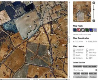
A prototype visualisation tool has been developed and applied to the Bet Bet Creek Catchment, Victoria. The purpose of the tool is to detect dryland salinity within a rural landscape, where users can draw a transect on a map, and subsequently generate a cross-sectional representation of the surface layer, predicted depth-to-water-table and confidence intervals of the error surface for ground water level.

Scaleable Vector Graphics (SVG) in conjunction with JavaScript was used to build the prototype, which can ultimately be accessible online by natural resource managers and the wider community. The tool, which integrates GIS data, and interfaces with hydrological models, is designed to be accessible and usable by a wide online user group. This paper focuses on the development of the tool, the underlying principles guiding its design, and the inclusion and communication of spatial uncertainty. As evaluation and user feedback are essential in determining its utility, we also outline proposed future testing of the prototype, with both modellers and natural resource managers.

1. INTRODUCTION

Technological advances in accessible computer platforms and increased computational power have significantly contributed towards a wealth of new data and modelling products. Increasingly, models are being used to simulate natural processes and inform policy and decision-making (Sarewitz, 2000). Visualisation is an effective way to help decision-makers understand the data inputs and outputs from complex process and predicative models.

Understanding of data and data uncertainty varies between scientist and decision-maker. While modellers may be comfortable expressing uncertainty values with probability equations, the same meaning may not be so clear to decision-makers. It is also recognised that without providing explicit uncertainty measures with an analysis, natural resource managers will assume the study is more reliable than warranted (Lemons, 1996). Visualisation tools enable scientists and decision-makers to collaboratively view and assess the results of model simulations and their significance, a process which helps the decision-maker minimise their time and maximise their understanding of an issue (Cliburn, 2002).

Primary Industries Research Victoria (PIRVic) is developing capability to handle data and model uncertainty and to communicate this information both internally and to stakeholders, clients and community groups. The research is designed to enhance the science skills and integration of two key disciplines in:

1. Developing higher quality hydrological models in which there is a greater understanding of inherent uncertainty within the model, and an improved ability to estimate the certainty of model output.

2. Developing enhanced visualisation techniques for communicating complex modelling outcomes to natural resource managers and the wider community to aid understanding and decision-making.

According to MacEachren et al (2005) “We lack methods for depicting uncertainty simultaneously with data and interacting with those depictions in ways that are understandable, useful and usable”. Nor, he claims do we have a thorough understanding of the factors which comprise successful uncertainty visualisation. Our research aims to provide wider-access to a series of hydrological modelling outputs, allowing the user to interact with a mapping interface and generate a cross-sectional profile of the surface and water

layers, displayed simultaneously with the associated error. Using maps as visualisation tools elevates them from simply presenting facts to a medium for exploration of potential relationships (MacEachren 1992). In this case, the interaction between the various modelled layers illustrates how the uncertainty surrounding each is likely to affect, or change the estimation of dryland salinity within an area. This research attempts to design a prototype system that conveys this information clearly and meaningfully to end users.

2. BACKGROUND: VISUALISING UNCERTAINTY

It is widely acknowledged that Geographical Information Systems (GIS) packages do not provide capability to incorporate or visualise uncertainty (Reinke et al, 2006). It is imperative to develop effective techniques to express uncertainty both within the GIS environment and all spatial products. The visualisation of uncertainty is not a new concept (Cliburn et al, 2002). However, there is much to be done to formalise successful techniques for many representation types. Early work focused on the manipulation of Bertin’s (1983) visual variables (location, size, value, texture, colour, orientation and shape) to indicate where data was less certain. Building on this technique was the adjustment of colour through saturation and/or hue, and the altering of opacity levels (Evans, 1997). More recent methods have implemented fuzzy boundaries to display uncertainty in continuous data (Lowell et al, 2007), while computing advances enabled animation to produce flickering maps to indicate discrepancies in data certainty (Fisher 1993). Another technique involved displaying only data deemed to be 95% reliable (Evans, 1997). These techniques have had mixed results. Animation through flickering received user feedback ranging from helpful to “really offensive” (Monmonier & Gluck, 1994) while the 95% reliable method was found to be disconnecting, by interfering in users geographical reference of the complete dataset (Evans 1997). Beard et al (1993) note that the inclusion of uncertainty information should not interfere with perception and understanding of the data, but this has proved to be quite challenging.

3. ONLINE GIS TOOLS & TECHNOLOGIES

GIS are a common, effective way of displaying and analysing spatial data. However, accessibility is restrictive; users typically require commercial software and the ability to operate it. Cartwright et al (2005) acknowledge the increased use of the World Wide Web as an efficient means for

disseminating GIS products for which there are a range of tools available both in proprietary and open standards.

SVG was chosen as the development tool largely for the extensibility and flexibility it provides. As an open standard, it is defined in XML, a universal structure for web documents, which allows for easy integration with other web applications. JavaScript is a dynamic scripting language commonly used in client-side web development to detect user responses. The client-side functionality of JavaScript enables a more responsive user experience. JavaScript can be integrated with SVG to leverage powerful mapping functionality and control dynamic interfaces, capturing user actions.

Recent spatial applications have seen the take-up of JavaScript and Java applets in developing and distributing packages over the Web. An example is CASE (Coastal Aquifer Salinity Evaluation), developed by Prathapar1. Designed for use by hydrologists, CASE simulates hydrological processes generated by pumping groundwater through specified aquifers, allowing the user to set the simulation parameters.

4. PROJECT AREA

The Bet Bet Creek Catchment was chosen as the study area for the prototype development. Located in north-central Victoria, approximately two hours from Melbourne, the region is the focus of the Upper Bet Bet targeted salinity project, a joint project of the local community and catchment management authority, the Victorian Government, and private industry. The region was selected to achieve key salinity outcomes through the planting of trees and control of salt, by monitoring groundwater levels, land use change and stream quality. The project aims to reduce groundwater recharge and minimise salt wash-off. To achieve this, an understanding of the hydrogeological processes that cause dryland salinity is required. A key feature of the project is monitoring of groundwater levels, stream quality, saline discharge and land use change2. The prototype is being applied to an actual geographic environment to demonstrate its usage within a real context and thus enhance communication and appeal to local natural resource managers and decision-makers. Error surfaces in relation to groundwater tables do not currently exist, so simulated data was 1 http://typhoon.mines.edu/zipfiles/case.htm 2 http://www.dpi.vic.gov.au/dpi/vro/ nthcenregn.nsf/pages/nthcen_lwm_bet

generated, based on the actual elevation of the area.

5. PRODUCT DEVELOPMENT 5.1 GIS Component

ArcGIS was used to process spatial data for transfer to SVG. Relevant datasets from the Victorian Corporate Geospatial Data Library (CGDL) such as landcover, hydrology and roads were clipped to the study area and projected to a common datum (GDA 1994 MGA Zone 54). A Perl script3 then converted each shapefile to SVG format. Within the SVG environment, aerial photographs were used as the base dataset of the tools mapping interface, while other surface layers such as elevation were also represented, to provide multiple views of the data. Checkboxes on the interface provide layer control. Currently, all converted shapefiles are stored within the SVG file, but potentially they could reside in a spatial database and be dynamically retrieved.

5.2 Modelling surfaces

Two fictitious surfaces were prepared for the study area. The first is a map of the depth-to-water table (DTW) (figure 2) and the second is an uncertainty estimate around the DTW map (figure 3).

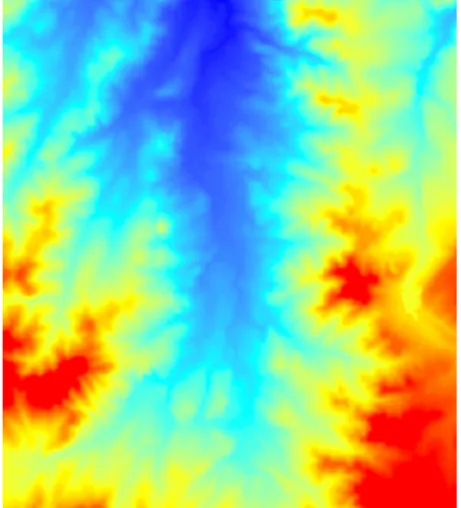
To prepare the DTW surface, a grid of points 200m apart was established across the area considered, and values between 0.2m and 10.0m – a realistic range for the Bet Bet catchment – assigned to each point. The values were assigned subjectively using an elevation map of the area as a guide (figure 4), i.e. higher elevations have a greater DTW than lower elevations. These points were then kriged (Burrough and McDonnell, 1998) using an exponential variogram and a maximum lag distance of 963m to produce the DTW surface (figure 2).

To prepare the uncertainty surface (figure 3), the same grid of points was used and a value between 0.4m and 2.2m assigned to each point. The assignment of values was also done semi-subjectively using the elevation surface (figure 4). However, for illustration purposes, uncertainty values were intentionally increased in the north-eastern quadrant, and decreased in the southern-central portion of the map. Values were then kriged as done previously to produce a continuous uncertainty surface.

3

Figure 2. Fictitious depth-to-watertable surface. Red values are the greatest depth (10m) and blue values are the lowest (0.2m).

Figure 3. Fictitious depth-to-watertable uncertainty surface. Red values have the greatest error (2.2m) and blue values have the lowest (0.2m).

Figure 4. Actual elevation surface for the area of interest. Red values have the highest elevation (450m M.S.L.) and blue values have the lowest

(290m).

5.3 Spatial Viewer

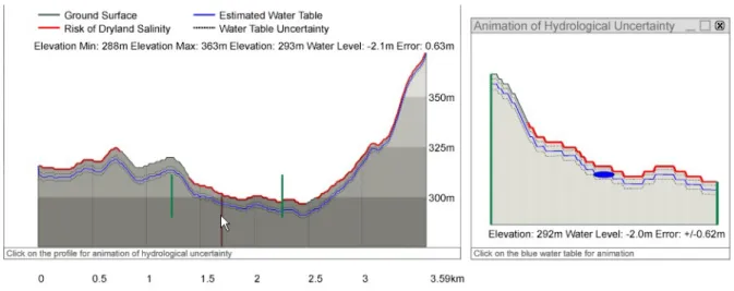
The interface consists of a main map area and linked overview map with tools for map interaction such as zooming and panning, and digitising tools for drawing a transect (figure 1). When a transect is drawn on the map a JavaScript bilinear function retrieves and interpolates the surrounding z-values from the DEM, to calculate the elevation along the surface line. Localised information is simultaneously retrieved for the depth-to-water table and error estimates. The combined information is then used to generate and display a cross-sectional profile on-screen (figure 5). The ground surface profile is shown (in grey), the estimated water table (in blue) and the error both above and below the water table (the dotted lines). Areas in which there is less than two metres between the upper error surface and the ground surface, which therefore poses a salinity risk, are indicated by the red line along the top of the cross-section. Horizontal grid markers below the cross-section indicate length in kilometres, while vertical graduated colour shows elevation in metres. The minimum and maximum elevation values are provided, while moving the mouse anywhere along the profile creates a red vertical marker and dynamically displays the elevation, water level and the associated uncertainty, at that point. The user is prompted to click on any point of interest within the cross-section to see a larger view of the area (figure 6) which is indicated by the green markers. This view can also be animated, with users clicking on the water table to see it rise and fall between error surfaces.

6. SOURCES OF UNCERTAINTY

Within the prototype there are three main sources of uncertainty: spatial data, modelling surfaces and JavaScript computations. Here, we will address each in some more detail.

1. The spatial data obtained from the CGDL represents landcover (or ecological vegetation class) is a grid format. For an area the size of Victoria, this may be sufficient, but when focusing on a region the size of the study area, it appears quite blocky and imprecise. In order to achieve an aesthetically appealing visualization, this layer underwent an automated raster to vector conversion. When draped over the aerial imagery, there are obvious discrepancies between the datasets. This may be attributed to a number of factors – different currency of the two datasets,

Figure 5 (left). Cross-sectional profile of the transect drawn on the map face, showing the ground surface(grey), the estimated water table (blue) the error (dotted black lines) and the risk of dryland salinity

(red); and Figure 6 (right). inset of area from Figure 5 (indicated by green lines) with animation option. scale and precision at which the data is

collected, or methods with which data is categorised. Lowell (2007) addresses the difficulties of determining what actually constitutes landcover, which is relevant in this case; “A single tree is not a forest, nor are ten trees, nor are even two hundred trees, if they are planted in a single line”.

2. The assumptions of modellers, complexity of natural systems, spatial data input (with its own inherent uncertainty) and natural variance, are all factors which contribute to model uncertainty (Adler et al, 2007). Compounding the issue, Buttenfield (1993) acknowledges that often with continuous spatial data true surfaces cannot be systematically determined, so discrepancy from true values cannot be known since actual values are unknown.

3. Lowell (2007) proposes that while it is difficult for model users to obtain reliability estimates of models this may be due to the fact that it is equally difficult for model developers to determine model reliability given all of these factors.

4. Finally JavaScript functionality takes the modelled surfaces (and their uncertainty) and interpolates the values to provide a subset analysis. Hunter et al (2005) posed the question how do you take spatial data with its limitations and metadata, generate complex modelling processes, apply spatial operations and categorically determine the uncertainty of the integrated product?

7. EVALUATION

Prior to commencing formal empirical evaluation and usability testing with the target user groups,

there are (we perceive) some notable strengths in the design and implementation of the prototype uncertainty tool. Firstly, as an online tool it can be easily accessed by natural resource managers and community groups. Secondly, it is interactive, allowing users to directly manipulate the interface by turning layers on and off, digitising, generating cross sectional profiles, and controlling animation sequences. McGranaghan (1993) suggests that interaction could be considered another visual variable, providing a more active and engaging experience for the user, allowing them to get to know the data, rather than merely observe. Thirdly, it is exploratory, allowing users to extract data (and associated uncertainty) specific to a location. End-users can drill down to farm level data. The combination of all of these elements means the tool lends itself well to being used in the context of a public participatory planning support system (Pettit & Nelson, 2004) to address the presence of dryland salinity at a property level, and also to stimulate broader discussion of the overall issue and promote an exchange of ideas.

Conversely, we have found there to be limitations with both aspects of the tool, and of the development language. As with most mapping products, showing large areas and a high level of detail are often mutually exclusive, and the prototype is no exception. Given the size of the study area, the maximum length of a transect drawn by the user, is about ten kilometres in length. Across this area, elevation may vary up to one hundred metres. Creating a cross section of this magnitude allows for little detail to be shown of the estimated water depth table and its associated error, which, at a maximum, never exceeds two metres above or below the estimated water table.

The appearance of the cross-sectional profile could be smoother, but achieving this involves a trade-off; increasing the precision and complexity of modelling surfaces would provide a greater level of detail and, in some instances, a smoother profile, but at the expense of storage, processing power and display time. Alternatively, dynamic generation and sizing of the profile window, based on the dimensions of the transect, would provide greater flexibility and improved appearance of the profile, but SVG does not lend itself easily to this type of functionality.

8. TESTING & FUTURE WORK

The next phase of the research will focus largely on testing the tool with natural resource managers and modellers. Testing will focus on:

1. Understanding of the overall product, and its usability.

2. Understanding of the uncertainty display and its meaning.

3. Understanding of how uncertainty impacts and/or potentially alters decisions made by natural resource managers.

4. Modellers’ feedback on how accurately the visualisation portrays and communicates uncertainty, and suggested improvements/ enhancements.

Primarily the tool’s functionality is as a visualisation interface to hydrological models, but potential exists to develop a more complete package. This could incorporate background information such as metadata, explanation of the model assumptions and construction, the logic behind the JavaScript computations and the associated limitations of the package. Potential also lies in developing the cross-sectional representation from 2D to 3D, however many question the need to use 3D representations when 2D will suffice (Slocum et al, 2002), being both simpler to construct and often, to interpret.

Finally, the prototype could be linked to other tools such as the Catchment Analysis Tool (PIRVIC, 2005) enabling users to understand the implications of error where inbuilt error uncertainty in visualisation products is the norm. 9. CONCLUSION

This paper has described the rationale underpinning the prototype and the technologies used to construct the tool. Multiple sources of uncertainty within the tool were explained to highlight the difficulties in quantifying the overall uncertainty of the package. Interactivity was

shown to be useful in creating an exploratory, participatory tool. Future evaluation is needed to determine its utility and useability. Ultimately, the value of the tool will be determined by the next phase of testing with natural resource managers and modellers, which will also largely determine where future improvements will be directed. The prototype demonstrates how collaborative research can benefit natural resource managers as modelling and visualisation scientists combine skills and knowledge to successfully communicate hydrological uncertainty to stakeholders.

This tool is one example of a visualisation technique well suited to representing Z-dimension data, where multiple sources of uncertainty are displayed, in context, alongside original data. We need to develop and evaluate a range of visualisation techniques and tools to communicate uncertainty specific to diverse spatial data types. These techniques and tools need to be made available so organisations can build on and progress the work of others and in turn share these tools with the wider community.

Just as the modelling community is harnessing increased computer processing power to develop complex models, visualisation scientists need to take full advantage of technology to create interactive, innovative maps and visualisation tools for future applications.

10. ACKNOWLEDGEMENTS

This project utilised free software provided by carto.net4. We gratefully acknowledge the use of these resources in developing the tool, which fast-tracked the process by building upon existing, proven technologies.

11. REFERENCES

Adler, P., R.C. Barrett, M.C. Bean, J.E. Birkhoff, Managing scientific and technical information in environmental cases, U.S. Institute for Environmental Conflict Resolution.

Accessed 2007. Available from: http://consensus.fsu.edu/ResourceCtr/sci_c ulture.pdf

Beard, K. and W. Mackaness (1993), Visual Access to data quality in Geographic Information Systems, Cartographica, 30(2&3), 37-45.

4

Bertin, J. (1983) Semiology of Graphics: Diagrams, networks, maps (translation from French 1967 edition by W.Berg). University of Wisconsin Press, Madison. Burrough, P., R. McDonnell, (1998) Principles of

Geographical Information Systems, Oxford University Press, Inc., New York.

Buttenfield, B.P. (1993), Representing data quality, Cartographica, 30(2), 1-7.

Cartwright, W., C. Pettit, A. Nelson and M. Berry (2005) Towards an understanding of how the ‘geographical dirtiness’ (complexity) of a virtual environment changes user perceptions of a space, paper presented at the International Congress on Modelling and Simulation Advances and Applications for Management and Decision Making (MODSIM05), Melbourne, Australia, December 12-15

Cliburn, D.C., J.J. Feddema, J.R. Miller and T.A. Slocum (2002), Design and evaluation of a decision support system in a water balance application, Computers & Graphics, 26(6) 931-949.

Evans, B.J., (1997), Dynamic display of spatial data-reliability: does it benefit the map user? Computers and Geosciences, 24(1) 1– 14.

Fisher, P.F., (1993), Visualising uncertainty in soil maps by animation, Cartographica, 30(2+3):20-27.

Hunter G., S. Hope, Z. Sadiq, A.Boin, M.Marinelli, A.N. Kealy, M, Duckham and R.J. Corner (2005), Next generation research issues in spatial data quality, presented at The National Biennial Conference of the Spatial Sciences Institute, Melbourne, Australia, September 2005.

Lemons, J. (1996) Scientific Uncertainty and Environmental Problem Solving, ed. Lemons, J., Cambridge MA, Blackwell Science, 1-11.

Lowell, K., K. Benke and C. Pettit (2007), Spatial considerations for uncertainty in hydrological modelling and implications for visualisation, presented at the Spatial Sciences Institute Conference, Hobart, Australia, May 14-18.

Lowell, K. (2007) Uncertainty in Landscape Models, presented at Place and Purpose: Spatial Models for Natural Resource Management and Planning, Bendigo, Australia, May 30-31.

MacEachren, A. (1992), Visualizing uncertain information, Cartographic Perspective, 13(4), 10–19.

MacEachren, A.M., A. Robinson, S. Hopper, S. Gardner, R. Murray, M. Gahegan and E. Hetzler (2005), Visualising geospatial information uncertainty: what we know and what we need to know, Cartography and GIS, 32(3), 139-160.

McGranaghan, M. (1993), A cartographic view of spatial data quality, Cartographica, 30(2&3), 8-19.

Monmonier, M. and M. Gluck (1994), Focus groups for design improvement in dynamic cartography, Cartography and GIS, 21(1), 37-47.

Pettit, C. and Nelson, A. (2004), Developing an Interactive Web Based Public Participatory Planning Support System for Natural Resource Management, Journal of Spatial Science, 49(1), 61-70.

PIRVIC (2005), Technical Manual Catchment Analysis Tool, Version 14, PIRVic Department of Primary Industries Victoria, 1-184.

Reinke. K., S. Jones and G. Hunter (2006), Implementation of a prototype toolbox for communicating spatial data quality and uncertainty using a wildfire risk example, Progress in Spatial Data Handling (12th presented at the International Symposium on Spatial Data Handling). Riedl, A., W. Kainz and G. Elmes, New York, Springer, 321–337.

Sarewitz, D., J.R. Pieke and J.B. Byerly (2000), Prediction in science and policy, Prediction, Science, Decision Making, and the Future of Nature, Washington D.C., Island Press. Slocum, T.A., D.C. Cliburn, J.J. Feddema and

J.R.Miller (2003), Evaluating the usability of a tool for visualizing the uncertainty of the future global water balance, Cartography and GIS, 30(4), 299-317.