This item was submitted to Loughborough’s Institutional Repository
(
https://dspace.lboro.ac.uk/
) by the author and is made available under the
following Creative Commons Licence conditions.
For the full text of this licence, please go to:
http://creativecommons.org/licenses/by-nc-nd/2.5/
Theorem 2: Ifx(t)is a real-valued signal,M1 = (a1; b1; c1; d1), M2 = (a2; b2; c2; d2), then 1u2 M 1u2M a1a21t2+ b41t1b22 2 + (a1b20 a4 2b1)2 (12) and the equality is achieved iff x(t) = (1=2)1=4exp(0((t 0 t0)2=22)), whereis an arbitrary real constant.
Proof: With the results of Lemma 2 and 3, we can obtain
1u2 M = 1E +1 01 juXM(u)j2du 0 u2M0 = 1E a2 +1 01 jtx(t)j2dt + b2 1 01 j!X(!)j2d! +jab(I30 I)] 0 a2t200 b2!020 2abt0!0
= a21t2+ b21!2+ jab(I30 I)
E 0 2abt0!0
= a21t2+ b21!2 (13)
becausex(t)is real, which means!0 = 0andI is real. Therefore, using (13) and the uncertainty relation in the FT domain, the spread in any LCT domain for a real signal is lower bounded by its spreads in the time and frequency domains, i.e.,
1u2
M a21t2+ b 2
41t2: (14)
For arbitrary two LCT domains we have
1u2 M 1u2M a211t2+ b 2 1 41t2 1 a221t2+ b 2 2 41t2 = (1t2)2a2 1a22+ b 2 1b22 16(1t2)2 + a 2 1b22+ b21a22 4 = a1a21t2+ b41t1b22 2 + (a1b20 a4 2b1)2 and the equality is achieved iffx(t)is a Gaussian signal.
IV. CONCLUSION
In this correspondence, we discuss the uncertainty relations in the LCT domain. A lower bound for complex signals in two LCT do-mains is derived, which can be achieved by a complex chirp signal with Gaussian envelope. Moreover, the tighter lower bound for real signals in two LCT domains given in [15] is also proven to hold for arbitrary LCT parameters based on the properties of moments in the LCT do-main. The uncertainty principle in the FrFT domain is a special case of the achieved results.
REFERENCES
[1] M. Moshinsky and C. Quesne, “Linear canonical transformations and their unitary representations,”J. Math. Phys., vol. 12, pp. 1772–1783, Aug. 1971.
[2] L. M. Bernardo, “ABCD matrix formalism of fractional Fourier op-tics,”Opt. Eng., vol. 35, no. 3, pp. 732–740, Mar. 1996.
[3] S. C. Pei and J. J. Ding, “Eigenfunctions of linear canonical transform,”
IEEE Trans. Signal Processing, vol. 50, no. 1, pp. 11–26, 2002. [4] R. Tao, L. Qi, and Y. Wang, Theory and Applications of the Fractional
Fourier Transform. Beijing: Tsinghua University Press, 2004. [5] H. M. Ozaktas, M. A. Kutay, and Z. Zalevsky, The Fractional Fourier
Transform With Applications in Optics and Signal Processing. New York: Wiley, 2000.
[6] L. B. Almeida, “The fractional Fourier transform and time-frequency representations,”IEEE Trans. Signal Processing, vol. 42, no. 11, pp. 3084–3091, 1994.
[7] B. Barshan, M. A. Kutay, and H. M. Ozaktas, “Optimal filters with linear canonical transformations,”Opt. Commun., vol. 135, pp. 32–36, 1997.
[8] K. K. Sharma and S. D. Joshi, “Signal separation using linear canon-ical and fractional Fourier transforms,”Opt. Commun., vol. 265, pp. 454–460, 2006.
[9] D. Mustard, “Uncertainty principle invariant under fractional Fourier transform,”J. Austral. Math. Soc. Ser. B, vol. 33, pp. 180–191, 1991. [10] H. M. Ozaktas and O. Aytur, “Fractional Fourier domains,”Signal
Pro-cessing, vol. 46, pp. 119–124, 1995.
[11] T. Alieva and M. J. Bastiaans, “On fractional Fourier transform mo-ments,”IEEE Signal Processing Letters, vol. 7, no. 11, pp. 320–323, 2000.
[12] S. Shinde and V. M. Gadre, “An uncertainty principle for real signals in the fractional Fourier transform domain,”IEEE Trans. Signal Pro-cessing, vol. 49, no. 11, pp. 2545–2548, 2001.
[13] C. Capus and K. Brown, “Short-time fractional Fourier methods for the time-frequency representation of chirp signals,”J. Acoust. Soc. Am, vol. 113, no. 6, pp. 3253–3263, 2003.
[14] A. Stern, “Uncertainty principles in linear canonical transform domains and some of their implications in optics,”J. Opt. Soc. Am. A, vol. 25, no. 3, pp. 647–652, 2008.
[15] K. K. Sharma and S. D. Joshi, “Uncertainty principles for real signals in linear canonical transform domains,”IEEE Trans. Signal Processing, vol. 56, no. 7, pp. 2677–2683, 2008.
A Multiplicative Algorithm for Convolutive Non-Negative Matrix Factorization Based on Squared Euclidean Distance
Wenwu Wang, Andrzej Cichocki, and Jonathon A. Chambers
Abstract—Using the convolutive nonnegative matrix factorization (NMF) model due to Smaragdis, we develop a novel algorithm for matrix decom-position based on the squared Euclidean distance criterion. The algorithm features new formally derived learning rules and an efficient update for the reconstructed nonnegative matrix. Performance comparisons in terms of computational load and audio onset detection accuracy indicate the ad-vantage of the Euclidean distance criterion over the Kullback–Leibler di-vergence criterion.
Index Terms—Audio object separation, convolutive nonnegative matrix factorization, multiplicative algorithm, squared Euclidean distance.
I. INTRODUCTION
Non-negative matrix factorization (NMF), an emerging technique for data analysis [1], [2], has found many potentially useful
appli-Manuscript received August 28, 2008; accepted January 27, 2009. First pub-lished March 10, 2009; current version pubpub-lished June 17, 2009. The associate editor coordinating the review of this manuscript and approving it for publica-tion was Dr. Mark J. Coates. This work was presented in part at the IEEE Inter-national Symposium on Signal Processing and Information Technology, Cairo, Egypt, 2007.
W. Wang is with the Centre for Vision, Speech and Signal Processing, De-partment of Electronic Engineering, University of Surrey, Guildford, GU2 7XH, U.K. (e-mail: [email protected]).
A. Cichocki is with the Laboratory for Advanced Brain Signal Processing, Brain Science Institute, RIKEN, Saitama, 351-0198, Japan (e-mail: cia@brain. riken.jp).
J. A. Chambers is with the Advanced Signal Processing Group, Department of Electronic and Electrical Engineering, Loughborough University, Loughbor-ough, Leics LE11 3TU, U.K. (e-mail: [email protected]).
Color versions of one or more of the figures in this paper are available online at http://ieeexplore.ieee.org.
Digital Object Identifier 10.1109/TSP.2009.2016881
cations in signal and image processing, e.g., [3]–[19]. For example, in audio signal processing, based on spectrogram factorization, NMF has been applied to music transcription [5], [9] and audio source separation [16]–[19]. The standard NMF model given in [1] has been shown to be satisfactory and sufficient in certain tasks provided that the spectral frequencies of the analyzed audio signal do not change dramatically over time, which is however not the case for many re-alistic audio signals. As a result, the single basis obtained via the standard NMF decomposition may not be adequate to capture the temporal dependency of the frequency patterns within the signal. Moreover, a single basis function is typically required for the rep-resentation of each note of a given instrument in music audio, and therefore a clustering step needs to be used for source separation of instruments playing melodies [20], [19] and [18]. However, as iden-tified by [18], it may be difficult to perform a reliable clustering in many situations.
To overcome these issues, the approaches of convolutive NMF (or similar methods called shifted NMF) have been introduced in [6]–[8], [13], [18], and [19]. As a common characteristic of these approaches, the data to be analyzed are modelled as a linear combination of a group of shifted matrices. However, the developed learning algorithms have different characteristics due to the various strategies adopted in their derivation or different applications being addressed. For example, a multiplicative learning algorithm has been developed in [6] and [7] for the adaptation of a criterion based on the Kullback–Leibler (KL) divergence, and no restrictions are enforced on the frequency resolution of the spectrogram. In [18], translated versions of a single basis function are used to represent the typical frequency spectrum of any notes belonging to a single music source, which however requires the spectrogram to be logarithmic in the frequency scale. In [19], the learning algorithms are developed based on explicit constraints of temporal continuity and sparseness of the signals.
The convolutive learning rules developed in [6] and [7] are essen-tially an extension of the multiplicative rules in [1] for the minimization of the KL error norm. However, no formal mathematical derivations are given therein. Moreover, although there are learning algorithms for the standard NMF [1] based on the Euclidean distance, few such algo-rithms have been proposed for the convolutive case. The aim of this cor-respondence is to address these issues. To this end, we formally derive a multiplicative algorithm for the gradient adaptation of the error norm measured by the squared Euclidean distance. In addition, we provide an efficient procedure for the update of the reconstructed data matrix at each iteration, which can considerably reduce the computational load required by existing algorithms in the literature. The original idea of this work has been presented in [10].
We have applied our proposed algorithm to the audio object sepa-ration problem (i.e., the detection of repeating patterns, or note events from music audio signals), which is one of the core issues underlying many applications in audio engineering such as music transcription, audio information retrieval, low bit-rate audio coding, and automatic auditory scene analysis. In order to show its general performance, we have compared the proposed algorithm with the methods in [6] and [11], respectively, in this application context. Our experimental results reveal its superior performance to that of the two benchmark methods, especially in terms of its computational efficiency and note detection accuracy.
The remainder of the correspondence is organized as follows. The next section briefly reviews the standard NMF and Smaragdis’ original work on convolutive NMF. The proposed convolutive NMF algorithm is described in detail in Section III. Section IV investigates the per-formance of the proposed algorithm using numerical experiments, and conclusions are drawn in Section V.
II. PRELIMINARIES
A. Standard NMF
Given anM 2 Nnonnegative matrixX 2 M2N+ , the goal of NMF is to find nonnegative matricesW 2 M2R+ andH 2 R2N+ , such that X WH, whereRis the rank of the factorization, generally chosen to be smaller thanM (orN), or akin to(M + N)R < MN, which results in the extraction of some latent features whilst reducing some redundancies in the input data. To findWandH, several error func-tions have been proposed [1]–[4], one of which, denotedL(1), is based on the squared Euclidean distance
( ^W; ^H) = arg min W;H L(W; H) = arg minW;H 1 2 X 0 ^X 2 F (1)
whereW^ andH^ are the estimated optimal values ofWandH,k1kF denotes the Frobenius norm, andX^ is given byX = WH:^ Alterna-tively, we can also minimize the error function based on the extended KL divergence ( ^W; ^H) = arg min W;H M m=1 N n=1 Dm;n (2)
whereDm;nis them; nth element of the matrixDgiven byD = X log[X ^X] 0 X + ^X, whereand denote the Hadamard (el-ement-wise) product and division, respectively. We are particularly in-terested in the multiplicative algorithm of Lee and Seung [1], [2] due to its simplicity. In matrix form, the algorithm for minimizing criterion (1) can be written as
Hq+1= Hq((Wq)TX) ((Wq)TWqHq) (3)
Wq+1= Wq(X(Hq+1)T) (WqHq+1(Hq+1)T) (4)
whereqis the iteration index, and(1)Tis the matrix transpose operator. These rules are easy to implement. In addition, a step-size parameter which is normally required for gradient algorithms [4], is not necessary in these rules.
B. Convolutive NMF
To take into account the potential dependency between the neigh-boring columns of the input data matrixX, the standard (instantaneous) NMF can be extended to a convolutive model [6]
^ X =
P 01
p=0
W(p)p!H (5)
whereW(p) 2 M2R+ ,p = 0; . . . ; P 0 1, are a set of basis matrices, H 2 R2N
+ is a weighting matrix, and p!
H shifts the columns ofHby pspots to the right, with the columns shifted in from outside the matrix set to zero. Effectively,X^ is now expressed as a sum of shifted ma-trix products. These column shifts are noncircular. Analogously, pH shifts the columns ofH bypspots to the left. These notations will also be used for the shifting operations of other matrices throughout the work. Note that,0!H = 0H = H. With the convolutive model, the temporal continuity possessed by many audio signals can be expressed more effectively in the time-frequency domain, especially for those sig-nals whose frequencies vary with time [6].
To find a decomposition with the form of (5), Smaragdis has further proposed multiplicative learning rules based on the extended KL diver-gence (2), which can be rewritten as
Hq+1= Hq(((Wq(p))TX p~q) ((Wq(p))T444)) (6)
Wq+1(p) = Wq(p)(( ~Xq(Hp!q+1)T) (4(Hp!q+1)T)) (7)
where444is anM 2 N matrix whose elements are all set to unity, ~
C. Motivations and Contributions of Our Work
Two technical issues in [6] are worth, however, further investigation. First, no formal mathematical derivation for (6) and (7) was provided. As a result, the theoretical analysis of its convergence performance may become difficult to achieve. Second, no learning rules were developed for convolutive NMF under the criterion (1). In this correspondence, we develop a novel algorithm by formally deriving the learning rules using the criterion (1). After comparisons with the KL divergence based criterion, we have observed that the Euclidean distance based criterion provides better performance for convolutive NMF in terms of computa-tional load and onset detection accuracy. To the best of our knowledge, it is probably the first study to address the performance difference be-tween algorithms based on the two criteria in this context. Another con-tribution in our work is using efficient recursions in the adaptation of the reconstructed nonnegative matrix for further reducing the computa-tional load of our algorithm, which can be readily applied to a category of similar algorithms. Note, that similar symbolic notations as those in [6] are used here for matrix shifts and convolutions, simply for making easy comparison between the algorithms.
III. A NOVELCONVOLUTIVENMF ALGORITHM
A. Derivation of the Learning Rules
We first derive the update rules forW(p). According to (5), we have the derivativeX^i;jwith respect to (w.r.t)Wm;n(p),
@ ^Xi;j @Wm;n(p) = @ p d Wi;d(p) p! Hd;j @Wm;n(p) = @ d Wi;d(p) p! Hd;j @Wm;n(p) = i;m p! Hn;j (8)
wherei;mis the Kronecker delta, and the right-bottom subscripts rep-resent the element indices of a matrix, e.g.,X^i;jis thei; jth element of the matrixX^. Similarly, according to (1) and (8), we have the deriva-tive ofLw.r.tWm;n(p), @L @Wm;n(p)= i j ( ^Xi;j0 Xi;j) @ ^ Xi;j @Wm;n(p) = j ( ^Xm;j0 Xm;j) p! Hn;j: (9)
Let the element-wise step-size1be
[W(p)]m;n= Wm;n(p) j
p!
Hn;jX^m;j
: (10)
Using (9) and (10), we can derive the adaptation equation ofWm;n(p)
as Wm;n(p)= Wm;n(p)0[W(p)]m;n@W@L m;n(p) (11) = Wm;n(p) 0 Wm;n(p) j p! Hn;jX^m;j j ( ^Xm;j0Xm;j) p! Hn;j (12)
1Note that, the selection of such a learning rate follows from the similar
rescaling operation used in [2], and the convergence of our proposed algorithm under such a learning rate can be proved similarly for the convolutive model.
= Wm;n(p)(X( p! H )T) m;n ( ^X(p!H )T)m;n: (13)
In matrix form, the update (13) can be written as (marked with iteration numberq)
Wq+1(p) = Wq(p)((X(Hp!q)T) ( ^Xq(Hp!q)T)) (14)
wherep = 0; . . . ; P 0 1. Similarly, using the gradient @L @Hm;n = j Wj;m(p)( p ^ Xj;n0 p Xj;n) (15)
we can obtain the update equation forHin matrix form as
Hq+1= Hq(((Wq+1(p))T pX ) ((Wq+1(p))TX p^q)): (16)
It is worth noting that (6) and (7) can be obtained using a similar deriva-tion method and the KL divergence.
B. Further Practical Improvements
1) Update ofH: It can be observed from (14) and (16) thatP + 1 matrices in total, i.e., a setP ofW(p),p = 0; . . . ; P 0 1, requires to be updated first, followed byH, at each iteration. Specifically,H is updated usingW(P 0 1), which is the last update in theP loop for updatingW(p). As a result, the update ofHcan be dominated by W(P 0 1). In order to mitigate this effect, as suggested in [6], we can first update allW(p),p = 0; . . . ; P 0 1, and then take the average of all the updates forH, that is
Hq+1= 1 P P 01 p=0 Hq(p) (17) whereHq(p)is given by Hq(p) = Hq(Wq+1(p)T pX ) (Wq+1(p)T pX^q): (18)
In contrast to (16), the update (17) also exploits the information from W(0); . . . ; W(P 0 2)[see (18)], which has the practical advantage of reducing the dominant effect ofW(P 0 1)for the update ofHq+1 in (16). Note in this correspondence, that (17) is an intuitive operation which is obtained empirically, rather than justified theoretically.
2) Update ofX^: From (16) and (14), it is clear that the updates of HandW(p)both rely on the update ofX^, which, on the other hand, depends on the instantaneous values ofW(p)andH, according to (5). This means thatX^ should be updated correspondingly once for each W(p)update. Nevertheless, updating the whole (5) is computationally demanding if only an individualW(p)has a new value. Therefore, instead of directly using (5), we use the following simpler formulation
^
Xq= ^Xq0Wq(p)Hp!q+ Wq+1(p)Hp!q (p = 0; . . . ; P 0 1) (19)
whereX^qis updated to accommodate the new values of eachW(p) (inside thePloops), and the initial value ofX^q(q > 1) in the right-hand side (RHS) of (19) is obtained at the end of the (q 0 1)th iteration (outside theP loops), when the recursions are completed. Forq = 1,
^
Xqin the RHS of (19) is still calculated via (5). In practice, we found
that the nonnegative property ofX^qmay not be guaranteed, due to the subtraction operation and small numerical errors. The small negative values can be prevented by using the following projection:
^ Xq
TABLE I
SUMMARY OF THEPROPOSEDALGORITHM: CONVNMF-ED
whereX^qi;j is thei; jth element of the matrixX^ at the iteration q, max(1)takes the maximum value of its arguments, andis a trivial constant, typically, = 1009in our implementation. The algorithm stops iterations when the following criterion is satisfied:
^ Xq+10 ^Xq F ^ Xq F < (21)
whereis a small constant.
C. Nonnegative Decomposition of Magnitude Spectra
In our problem, the nonnegative matrixXis generated as the magni-tude spectra of the input audio data. For a signal withLsamples, using aT-point short-term Fourier transform (STFT), it can be segmented toKframes, whereK = b(L 0 T )=c,is the time shift between the adjacent windows andb1cis an operator taking the maximum in-teger no greater than its argument. Concatenating the absolute value of the spectrum of each frame, we can generateXwith a dimension of (T=2 + 1) 2 K(see details in [9]). The proposed algorithm can be summarized in Table I, whereW(p)andH(p)are typically initial-ized with random nonnegative elements. For convenience, we name it as ConvNMF-ED (i.e., convolutive NMF based on squared Euclidean distance).
Upon convergence of the algorithm,Xis decomposed into the con-volution ofPnonnegative matrices, denoted asWo(p) 2 (T =2+1)2R+ and Ho 2 R2K+ , i.e., the corresponding local optimum values of W(p)andH, respectively. AndHo contains the bases of the tem-poral patterns whileWo(p)contains the frequency patterns of the orig-inal signal. All the set ofP Wo(p)matrices together contain both fre-quency and temporal information of the time-frefre-quency patterns (i.e., audio objects) of the original audio signal.
D. Comparisons to Existing Methods
IfP = 1, ConvNMF-ED reduces to a standard NMF algorithm sim-ilar to that represented by (3) and (4) with the difference in the update ofX^q. IfP > 1, its computational load is approximatelyPtimes that of the standard NMF. ConvNMF-ED is different from Smaragdis’ al-gorithm [6] in steps 3–4 (see Table I), whereWq(p),X^qandHq(p) in [6] are instead updated by (7), (5) and (6), respectively. As a result, compared with [6], ConvNMF-ED requires(2RP 04R+P +2)MN fewer element operations (multiplications and additions) in each iter-ation. We also consider a faster version of Smaragdis’ algorithm [6], denoted as ConvNMF-KL, which is similar to [6] except thatX^q is updated using (19) and (20), instead of (5). Apart from its higher com-putational efficiency, ConvNMF-KL has very similar performance to [6]. Therefore, it is also used as an alternative to [6] in our simulations. Although the algorithm in [7] uses the same learning rules as those in [6], it is a supervised speech separation approach using additional constraints from the application domain. Making direct comparisons
to [7] is not straightforward; therefore, it is not explored further in this work.
SNMF2D [11], [12] considers a two-dimensional deconvolution scheme, together with sparseness constraints. We will examine the most related learning rules based on the least squares (LS) criterion in [12], i.e., SNMF2D-LS. In contrast, SNMF2D-LS uses the shifted versions of Wq and Hq at all time lags p = 0; . . . ; P 0 1, for updating Wq(p) and Hq(p) with an individual time lag at each iteration. For example, according to [11], the update ofH in (16) may be written as
Hq+1= Hq[(Wq+1(0)T 0X + 1 1 1 + Wq+1(P 0 1)T P 01X )]
[(Wq+1(0)TX 0^q) + 1 1 1 + (Wq+1(P 0 1)T P 01X^q )]: (22) The resulting representation ofWo(p)andHo using SNMF2D-LS has actually broken the structure of audio objects, i.e., the time-frequency signature in the spectrogram has been shifted more than it actually requires. As a result, it becomes difficult to detect the event or onset directly fromWo(p)andHo(as shown in our experi-ments in Section IV). Furthermore, SNMF2D-LS is computationally much more expensive, as compared with both ConvNMF-ED and ConvNMF-KL. The time required for computing (22) would be approximately P 0 1 times than that for computing (16). These observations will be further confirmed in numerical experiments.
IV. NUMERICALEXPERIMENTS
In this section, we study numerically the performance of Con-vNMF-ED in the context of audio object detection,2 and perform
comparisons with ConvNMF-KL, SNMF2D-LS, and Smaragdis’ algorithm [6].
A. Music Audio
Two music audio signals with each containing repeating musical notes G4 and A3 played by a guitar are mixed together. The mixed signal is approximately 6.8 s sampled atfs = 22050 Hz. Note, that for illustrative purpose, the signals used in this section are relatively simple, however, realistic audio signals have also been tested in this work, see, e.g., Section IV-D. Some parameters used in the experi-ments are set as:T = 4096,P = 105,R = 2, = 0:0001. The described algorithms ConvNMF-ED and ConvNMF-KL, together with SNMF2D-LS,3were all applied to decomposeX, whereW(p)andH
are the absolute values of random matrices with elements drawn from a
2Numerical examples for applying the proposed algorithm to artificial audio
signals containing audio patterns whose frequency changes linearly with time have been shown in [10], where we have shown the failure of the standard NMF for such a scenario, and the advantage of our proposed algorithm.
3The MATLAB code of the SNMF2D algorithm was downloaded from
Morup’s webpage [14]. In our evaluations, the 2-D deconvolution is reduced to one dimension by setting = 0. The convolutional frame lengthwas held identical toPused in ConvNMF-KL and ConvNMF-ED in all experiments.
Fig. 1. Decomposition result ofXusing the proposed ConvNMF-ED algo-rithm. (a) is the plot of magnitude spectrum matrixXof the music audio signal. (b) and (c) are the plots of the rows of the factorizedH . (d) and (e) are the plots of the columns of the factorizedW (p)as a collection for allp = 0; . . . ; 104, where (d) represents time-frequency signature of note G4, while (e) denotes note A3.
Fig. 2. Decomposition result ofXusing the ConvNMF-KL algorithm. (a) is the plot of magnitude spectrum matrixXof the music audio signal. (b) and (c) are the plots of the rows of the factorizedH . (d) and (e) are the plots of the columns of the factorizedW (p)as a collection for allp = 0; . . . ; 104, where (d) represents the time-frequency signature of note A3, while (e) denotes note G4. Note that, the decomposedW andH by ConvNMF-KL differ from those by the ConvNMF-ED algorithm with a permutation ambiguity, which is inherent due to the signal model considered, although the ambiguity does not always occur in many of our random tests.
standardized Gaussian probability density function. All tests were run on a computer whose CPU speed is 1.8 GHz.
Figs. 1–3 show the decomposition results of these algorithms, re-spectively. In all these algorithms, plot (a) is the spectrogram matrix X. Plots (b) and (c) visualize the first and second row ofHo, and plots (d) and (e) visualize the first and second column ofWo(p)for the collection ofp. We can observe from these figures that the per-formance of ConvNMF-ED is approximately identical to that of Con-vNMF-KL, except for a difference in the permutation. The notes G4 and A3 were separated correctly by both algorithms, whereWo(p) represents the magnitude spectrum of the notes, whileHodenotes the onset locations of the notes. However, the SNMF2D-LS algorithm does not correctly identify the note events. For example, it can be seen from Fig. 3(b) and (c) that, after the convergence of the algorithm, the onset locations inHohave been actuallyover-shifted, i.e., shifted more than
Fig. 3. Decomposition result ofXusing the algorithm SNMF2D-LS. (a) is the plot of magnitude spectrum matrixXof the music audio signal. (b) and (c) are the plots of the rows of the factorizedH . (d) and (e) are the plots of the columns of the factorizedW (p)as a collection for allp = 0; . . . ; 104, where (d) represents the time-frequency signature of note G4, while (e) denotes note A3.
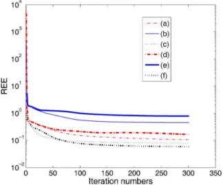
Fig. 4. Convergence comparison between the algorithms ConvNMF-ED (plots (a) and (d)), ConvNMF-KL (plots (b) and (e)), and SNMF2D-LS (plots (c) and (f)). Two random tests were performed for each algorithm withT = 256(plots (a) (b) and (c)), and 1024 (plots (d) (e) (f)) respectively.
TABLE II
COMPARISON OFCOMPUTINGTIMEREQUIRED FOR THEALGORITHMS RUNNING100 ITERATIONS. FOREACHT,THETIMECONSUMED
(INSECONDS) WASAVERAGEDOVER50 RANDOMTESTS
is required. As a consequence,Ho does not reveal the correct onset locations. Moreover, the magnitude spectrum of the notes described byWo(p)is less accurate than obtained by ConvNMF-KL and Con-vNMF-ED.
B. Convergence Performance
In this section, we compare numerically the convergence perfor-mance of the three algorithms. We perform two random tests for each
TABLE III
COMPARISON OFTP=FPFORNOTEONSETDETECTIONBETWEEN THETHREEALGORITHMS. FOREACHT,THERESULTWASAVERAGED OVER50 RANDOMREALIZATIONS. THEVALUES OFTP AREALSOSHOWN INBRACKETS.
algorithm withTset to 256 and 1024, respectively, and run each algo-rithm for 300 iterations. The evolution of the relative estimation error (REE) versus iteration number is drawn in Fig. 4, where REE is defined as
REE=
X 0 ^X
F
kXkF : (23)
This performance index is relatively less sensitive to the signal dynamics as compared with the absolute estimation error due to the adopted normalization. All the three algorithms were initialized randomly with the same starting points. The three algorithms have very similar convergence behavior, with SNMF2D-LS having lowest REE, followed by ConvNMF-ED and ConvNMF-KL.
C. Computational Load
To compare the computational complexity of the proposed algorithm with that of ConvNMF-KL, SNMF2D-LS and the algorithm in [6], we ran each algorithm 50 times for eachT, whereT was set to be 256, 512, 1024, 2048, and 4096, respectively. We measured the com-puting time required for 100 iterations. All the algorithms were ini-tialized randomly. Other parameters remained the same as those in Section IV-A. The average results over 50 tests for each algorithm are listed in Table II. More specifically, if we further average the results over differentT, the reductions of computing load of ConvNMF-ED as compared with ConvNMF-KL, SNMF2D-LS and Smaragdis’ algo-rithm in [6] are respectively 13%, 47%, and 51%. Clearly, the proposed algorithm ConvNMF-ED is the most efficient algorithm. WhenT be-comes larger or the signal to be analyzed bebe-comes longer, the advan-tage of ConvNMF-ED becomes more significant. This numerical result supports our theoretical analysis results in Section III-D.
D. Audio Object Separation Accuracy
In order to evaluate the convolutive NMF algorithms more objec-tively, it can be useful to measure the accuracy of the detected note events from Ho orWo(p)that is obtained using those algorithms. Here, we use the same peak-picking algorithm described [9] to detect the note onsets fromHo. The threshold used for peak-picking was set to 0.4 and held constant for all the tests. We evaluate the performance using the ratio between the percentage of true positives (i.e., the number of correct detections relative to that of total existing onsets, denoted as TP for brevity) and the percentage of the false positives (i.e., the number of erroneous onsets relative to that of the total detected onsets, denoted as FP for brevity) [21], i.e., TP=FP. A higher value of TP=FP indicates a relatively better performance. A detected note is considered to be a true positive if it falls into one analysis window within the orig-inal onset. Otherwise, it is considered as a false positive. In practice, there may exist a few missing notes that are not detected at all, which nevertheless does not affect the accuracy of evaluation using TP=FP. A subset of a commercial music audio database was used for the eval-uation, for which 25 testing signals, each containing various numbers of notes, were used [15]. For each signal,T was set to be 256, 512, 1024, 2048, and 4096, respectively, and 50 random realizations were run for eachT. Table III shows the average results of TP=FP, with TP also listed in the brackets. It can be seen from these figures that
SNMF2D-LS almost totally fails for onset detections of note events in the signals. This is not surprising regarding the discussion we had earlier in Sections III-D and IV-A. In contrast to both SNMF2D-LS and ConvNMF-KL, the proposed algorithm ConvNMF-ED provides the better decompositions that are particularly suitable for note onset detection.
V. CONCLUSION
A new multiplicative learning algorithm for convolutive NMF has been presented. The algorithm features novel learning rules derived from the squared Euclidean distance, together with an efficient method for computing the estimate of the low-rank approximation. The pro-posed algorithm has advantages over both Smaragdis’ algorithm and the algorithm by Schmidt and Morup, in the context of audio object sep-aration and note onset detection, in terms of the performance measure-ment of computational complexity and detection accuracy. The pro-posed algorithm can be a useful tool for a wide range of applications including the analysis of complex auditory scenes.
ACKNOWLEDGMENT
The authors would like to thank the associate editor and the anony-mous reviewers for their constructive comments.
REFERENCES
[1] D. D. Lee and H. S. Seung, “Learning the parts of objects by non-negative matrix factorization,”Nature, vol. 401, pp. 788–791, 1999. [2] D. D. Lee and H. S. Seung, “Algorithms for non-negative matrix
factor-ization,” inAdvances in Neural Information Processing. Cambridge, MA: MIT Press, 2001, vol. 13.
[3] P. O. Hoyer, “Non-negative matrix factorization with sparseness con-straints,”J. Mach. Learn. Res., no. 5, pp. 1457–1469, 2004. [4] A. Cichocki, R. Zdunek, and S. Amari, “Csiszar’s divergences for
non-negative matrix factorization: family of new algorithms,”Springer Lec-ture Notes in Comput. Sci., vol. 3889, pp. 32–39, 2006.
[5] P. Smaragdis and J. C. Brown, “Nonnegative matrix factorization for polyphonic music transcription,” inProc. IEEE Int. Workshop Applica-tions Signal Process. Audio Acoustics, New Paltz, NY, Oct. 2003, pp. 177–180.
[6] P. Smaragdis, “Non-negative matrix factor deconvolution, extraction of multiple sound sources from monophonic inputs,” inProc. 5th Int. Conf. Independent Component Analysis Blind Signal Separation, Granada, Spain, Sep. 22–24, 2004, vol. LNCS 3195, Lecture Notes on Computer Science, pp. 494–499.
[7] P. Smaragdis, “Convolutive speech bases and their application to super-vised speech separation,”IEEE Trans. Audio Speech Lang. Process., vol. 15, no. 1, pp. 1–12, 2007.
[8] P. D. O’Grady and B. A. Pearlmutter, “Convolutive non-negative ma-trix factorisation with a sparseness constraint,” inProc. IEEE Int. Work-shop Machine Learning Signal Process., Maynooth, Ireland, Sep. 6–8, 2006, pp. 427–432.
[9] W. Wang, Y. Luo, S. Sanei, and J. A. Chambers, “Non-negative matrix factorization for note onset detection of audio signals,” inProc. IEEE Int. Workshop Machine Learning Signal Process., Maynooth, Ireland, Sep. 6–8, 2006, pp. 447–452.
[10] W. Wang, “Squared Euclidean distance based convolutive non-negative matrix factorization with multiplicative learning rules for audio pattern separation,” inProc. IEEE Int. Symp. Signal Process. Info. Tech., Cairo, Egypt, Dec. 15–18, 2007.
[11] M. N. Schmidt and M. Morup, “Nonnegative matrix factor 2-D de-convolution for blind single channel source separation,” inProc. 6th Int. Conf. Independent Component Analysis Blind Signal Separation, Charleston, SC, 2006, pp. 700–707.
[12] M. Morup and M. N. Schmidt, “Sparse non-negative matrix Factor 2-D deconvolution,” Technical Univ., Denmark, 2006.
[13] M. Morup, K. H. Madsen, and L. K. Hansen, “Shifted non-negative matrix factorization,” inProc. IEEE Int. Workshop Machine Learning Signal Process., Maynooth, Ireland, Sep. 6–8, 2007, pp. 427–432. [14] M. Morup, 2007 [Online]. Available: http://www.mortenmorup.dk/
index_files/Page368.htm
[15] W. Wang, 2008 [Online]. Available: http://personal.ee.surrey.ac.uk/ Personal/W.Wang/demondata.html
[16] B. Wang and M. D. Plumbley, “Musical audio stream separation by non-negative matrix factorization,” inProc. DMRN Summer Conf., Glasgow, Jul. 23–24, 2005.
[17] R. M. Parry and I. Essa, “Incorporating phase information for source separation via spectrogram factorization,” in Proc. IEEE Int. Conf. Acoust., Speech, Signal Process., Honolulu, HI, Apr. 15–20, 2007, vol. 2, pp. 661–664.
[18] D. FitzGerald, M. Cranitch, and E. Coyle, “Sound source separation using shifted non-negative tensor factorization,” inProc. IEEE Int. Conf. Acoust., Speech, Signal Process., 2006, vol. V, pp. 653–656. [19] T. Virtanen, “Monaural sound source separation by non-negative
matrix factorization with temporal continuity and sparseness crite-rion,”IEEE Trans. Audio, Speech, Lang. Process., vol. 15, no. 3, pp. 1066–1074, Mar. 2007.
[20] M. Casey and A. Westner, “Separation of mixed audio sources by inde-pendent subspace analysis,” inProc. Int. Comput. Music Conf., Berlin, Germany, Aug. 2000, pp. 154–161.
[21] J. P. Bello, L. Daudet, S. A. Abdallah, C. Duxbury, M. Davies, and M. B. Sandler, “A tutorial on onset detection in musical signals,”IEEE Trans. Speech Audio Process., vol. 13, no. 5, pp. 1035–1047, Sep. 2005.
OFDM Joint Data Detection and Phase Noise Cancellation for Constant Modulus Modulations
Yu Gong and Xia Hong
Abstract—This correspondence proposes a new algorithm for the OFDM joint data detection and phase noise (PHN) cancellation for con-stant modulus modulations. We highlight that it is important to address the overfitting problem since this is a major detrimental factor impairing the joint detection process. In order to attack the overfitting problem we propose an iterative approach based on minimum mean square prediction error (MMSPE) subject to the constraint that the estimated data symbols have constant power. The proposed constrained MMSPE algorithm (C-MMSPE) significantly improves the performance of existing approaches with little extra complexity being imposed. Simulation results are also given to verify the proposed algorithm.
Index Terms—Constant modulus modulation, OFDM, phase noise can-cellation.
I. INTRODUCTION
The phase noise (PHN) in an orthogonal-frequency-division multi-plexing (OFDM) system arises from the imperfections at the receiver’s
Manuscript received August 26, 2008; accepted February 06, 2009. First ver-sion published March 21, 2009; current verver-sion published June 17, 2009. The associate editor coordinating the review of this manuscript and approving it for publication was Dr. Biao Chen.
The authors are with the School of Systems Engineering, The Univer-sity of Reading, Reading, RG6 6AY, U.K. (e-mail: [email protected]; [email protected]).
Color versions of one or more of the figures in this correspondence are avail-able online at http://ieeexplore.ieee.org.
Digital Object Identifier 10.1109/TSP.2009.2018362
oscillator, damaging the orthogonality among subcarriers [1], [2]. A typical PHN consists of two parts: the common PHN and the random PHN [3]. Most existing PHN cancellation algorithms (e.g., [3] and [4]) mainly consider the common PHN which is an averaging effect over the OFDM transmission and can be mitigated with the help of pilot symbols. The random PHN, on the other hand, is much more difficult to handle as it varies from one symbol to another even for slowly fading channels. Recently, a family of algorithms for joint data detection and PHN cancellation based on the probabilistic approach of variational in-ference have been proposed [5].
In general, a joint estimation process may suffer from the “overfit-ting” problem so that the estimate is too close to the received samples and fits into the noise. The overfitting problem is particularly serious in the joint OFDM data detection and PHN cancellation. This is because for an OFDM symbol withNsubcarriers, there areNdata symbols and NPHN to be determined from2Nobservations includingNfrom the receiving data model and anotherNfrom the PHN model. On another front, the PHN must be mitigated at every symbol since it varies from one symbol to another. This describes a very special case of parameter estimation problem: unlike the classic parameter estimation whereby the estimates can be improved by increasing the number of data sam-ples, here the number of unknown parameters (i.e., the symbols and PHN) always equals the number of the “observation” samples, making it particularly vulnerable to overfitting which thus must be carefully handled as otherwise the whole joint process may be invalidated.
We note that, although it was not explicitly identified, the algorithms described in [5] are in fact equivalent to the Bayesian regularization utilizing the Gaussian distributions as the priors, a common method to combat overfitting [6]. This, however, may not be sufficiently effective for the OFDM PHN cancellation. In our recent correspondence [7] and further in [8], we proposed a new joint data detection and PHN can-cellation algorithm based on minimum mean square prediction error (MMSPE), where the hard decision is applied to the symbol estimates at the end of each iteration. The hard decision process can effectively filter the noise out of the symbol estimates and remove the associated un-certainties due to the overfitting which would otherwise be carried for-ward over the iterations. However, the hard decision imposes as a non-linear constraint on the iterative procedure which may sometimes be too strong such that some symbol estimates are forced into the wrong direc-tion over the iteradirec-tions, resulting in performance loss. As will be shown in the simulation later in this correspondence, the MMSPE algorithm has close performance to, if not worse than, those proposed in [5] when the SNR is high (in which case there is little noise to be removed and the negative effect of the hard decision becomes more dominant). This motivates us to explore new methods to combat overfitting problem.
In this correspondence, we focus on the OFDM system with constant modulus modulations such as the PSK. Embedding the deterministica prioriinformation from the modulation that the data symbol must have constant power into the MMSPE cost function as a constraint, we pro-pose a constrained MMSPE (C-MMSPE) algorithm to jointly detect the data symbol and cancel the PHN. The C-MMSPE algorithm can better handle the overfitting and has significantly superior performance to both the MMSPE algorithm and the algorithms described in [5]. The idea of using constant modulus has been well understood in many com-munications applications such as the Godard blind equalization [9], but this is the first time to be applied to the OFDM PHN cancellation. Al-though in general any prior information about the system, especially deterministic knowledge, should greatly help to improve the model-ling performance, it usually leads to some complicated constrained op-timization problems with large computational complexity. Luckily in the case of the OFDM PHN cancellation, we will show that the derived