Lower Bound Techniques for Data Structures
by
Mihai Pˇ
atra¸scu
Submitted to the Department of
Electrical Engineering and Computer Science
in partial fulfillment of the requirements for the degree of
Doctor of Philosophy
at the
MASSACHUSETTS INSTITUTE OF TECHNOLOGY
September 2008
c
Massachusetts Institute of Technology 2008. All rights reserved.
Author . . . .
Department of
Electrical Engineering and Computer Science
August 8, 2008
Certified by . . . .
Erik D. Demaine
Associate Professor
Thesis Supervisor
Accepted by . . . .
Professor Terry P. Orlando
Chair, Department Committee on Graduate Students
Lower Bound Techniques for Data Structures
by
Mihai Pˇ
atra¸scu
Submitted to the Department of Electrical Engineering and Computer Science on August 8, 2008, in partial fulfillment of the
requirements for the degree of Doctor of Philosophy
Abstract
We describe new techniques for proving lower bounds on data-structure problems, with the following broad consequences:
• the first Ω(lgn) lower bound for any dynamic problem, improving on a bound that had been standing since 1989;
• for static data structures, the first separation between linear and polynomial space. Specifically, for some problems that have constant query time when polynomial space is allowed, we can show Ω(lgn/lg lgn) bounds when the space is O(n·polylogn). Using these techniques, we analyze a variety of central data-structure problems, and obtain improved lower bounds for the following:
• the partial-sums problem (a fundamental application of augmented binary search trees); • the predecessor problem (which is equivalent to IP lookup in Internet routers);
• dynamic trees and dynamic connectivity; • orthogonal range stabbing.
• orthogonal range counting, and orthogonal range reporting; • the partial match problem (searching with wild-cards); • (1 +)-approximate near neighbor on the hypercube; • approximate nearest neighbor in the `∞ metric.
Our new techniques lead to surprisingly non-technical proofs. For several problems, we obtain simpler proofs for bounds that were already known.
Thesis Supervisor: Erik D. Demaine Title: Associate Professor
Acknowledgments
This thesis is based primarily on ten conference publications: [84] from SODA’04, [83] from STOC’04, [87] from ICALP’05, [89] from STOC’06, [88] and [16] from FOCS’06, [90] from SODA’07, [81] from STOC’07, [13] and [82] from FOCS’08. It seems appropriate to sketch the story of each one of these publications.
It all began with two papers I wrote in my first two undergraduate years at MIT, which appeared in SODA’04 and STOC’04, and were later merged in a single journal version [86]. I owe a lot of thanks to Peter Bro Miltersen, whose survey of cell probe complexity [72] was my crash course into the field. Without this survey, which did an excellent job of taking clueless readers to the important problems, a confused freshman would never have heard about the field, nor the problems. And, quite likely, STOC would never have seen a paper proving information-theoretic lower bounds from an author who clearly did not know what “entropy” meant.
Many thanks also go to Erik Demaine, who was my research advisor from that freshman year until the end of this PhD thesis. Though it took years before we did any work together, his unconditional support has indirectly made all my work possible. Erik’s willingness to pay a freshman to do whatever he wanted was clearly not a mainstream idea, though in retrospect, it was an inspired one. Throughout the years, Erik’s understanding and tolerance for my unorthodox style, including in the creation of this thesis, have provided the best possible research environment for me.
My next step would have been far too great for me to take alone, but I was lucky enough to meet Mikkel Thorup, now a good friend and colleague. In early 2004 (if my memory serves me well, it was in January, during a meeting at SODA), we began thinking about the predecessor problem. It took us quite some time to understand that what had been labeled “optimal bounds” were not optimal, that proving an optimal bound would require a revolution in static lower bounds (the first bound to beat communication complexity), and to finally find an idea to break this barrier. This 2-year research journey consumed us, and I would certainly have given up along the way, had it not been for Mikkel’s contagious and constant optimism, constant influx of ideas, and the many beers that we had together.
This research journey remained one of the most memorable in my career, though, unfor-tunately, the ending was underwhelming. Our STOC 2006 [89] paper went largely unnoticed, with maybe 10 people attending the talk, and no special issue invitation. I consoled myself with Mikkel’s explanation that ours had been paper with too many new ideas to be digested soon after publication.
Mikkel’s theory got some support through our next joint paper. I proposed that we look at some lower bounds via the so-called richness method for hard problems like partial match or nearest neighbor. After 2 years of predecessor lower bounds, it was a simple exercise to obtain better lower bound by richness; in fact, we felt like we were simplifying our technique for beating communication complexity, in order to make it work here. Despite my opinion that this paper was too simple to be interesting, Mikkel convinced me to submit it to FOCS. Sure enough, the paper was accepted to FOCS’06 [88] with raving reviews and a special issue invitation. One is reminded to listen to senior people once in while.
After my initial interaction with Mikkel, I had begun to understand the field, and I was able to make progress on several fronts at the same time. Since my first paper in 2003, I kept working on a very silly dynamic problem: prove a lower bound for partial sums in the bit-probe model. It seemed doubtful that anyone would care, but the problem was so clean and simple, that I couldn’t let go. One day, as I was sitting in an MIT library (I was still an undergraduate and didn’t have an office), I discovered something entirely unexpected. You see, before my first paper proving an Ω(lgn) dynamic lower bound, there had been just one technique for proving dynamic bounds, dating back to Fredman and Saks in 1989. Everybody had tried, and failed, to prove a logarithmic bound by this technique. And there I was, seeing a clear and simple proof of an Ω(lgn) bound by this classic technique. This was a great surprise to me, and it had very interesting consequences, including a new bound for my silly little problem, as well as a new record lower bound in the bit-probe model. With the gods clearly on my side (Miltersen was on the PC), this paper [87] got the Best Student Paper award at ICALP.
My work with Mikkel continued with a randomized lower bound for predecessor search (our first bound only applied to deterministic algorithms). We had the moral obligation to “finish” the problem, as Mikkel put it. This took quite some work, but in the end, we succeeded, and the paper [90] appeared in SODA’07.
At that time, I also wrote my first paper with Alex Andoni, an old and very good friend, with whom I would later share an apartment and an office. Surprisingly, it took us until 2006 to get our first paper, and we have only written one other paper since then, despite our very frequent research discussions over beer, or while walking home. These two papers are a severe underestimate of the entertaining research discussions that we have had. I owe Alex a great deal of thanks for the amount of understanding of high dimensional geometry that he has passed on to me, and, above all, for being a highly supportive friend.
Our first paper was, to some extent, a lucky accident. After a visit to my uncle in Philadelphia, I was stuck on a long bus ride back to MIT, when Alex called to say that he had some intuition about why (1 +ε)-approximate nearest neighbor should be hard. As always, intuition is hard to convey, but I understood at least that he wanted to think in very high dimensions, and let the points of the database be at constant pairwise distance. Luckily, on that bus ride I was thinking of lower bounds for lopsided set disjointness (a problem left open by the seminal paper of Miltersen et al. [73] from STOC’95). It didn’t take long after passing to realize the connection, and I was back on the phone with Alex explaining how his construction can be turned in a reduction from lopsided set disjointness to nearest neighbor. Back at MIT, the proof obviously got Piotr Indyk very excited. We later merged with another result of his, yielding a FOCS’06 paper [16]. Like in the case of Alex, the influence that Piotr has had on my thinking is not conveyed by our number of joint papers (we only have one). Nonetheless, my interaction with him has been both very enjoyable and very useful, and I am very grateful for his help.
My second paper with Alex Andoni was [13] from FOCS’08. This began in spring 2007 as a series of discussions between me and Piotr Indyk about approximate near neighbor in
solution. By the summer of 2007, I had made up my mind that we had to seek an asymmetric communication lower bound. That summer, both I and Alex were interns at IBM Almaden, and I convinced him to join on long walks on the beautiful hills at Almaden, and discuss this problem. Painfully slowly, we developed an information-theoretic understanding of the best previous upper bound, and an idea about how the lower bound should be proved.
Unfortunately, our plan for the lower bound led us to a rather nontrivial isoperimetric inequality, which we tried to prove for several weeks in the fall of 2007. Our proof strategy seemed to work, more or less, but it led to a very ugly case analysis, so we decided to outsource the theorem to a mathematician. We chose none other than our third housemate, Dorian Croitoru, who came back in a few weeks with a nicer proof (if not lacking in case analysis).
My next paper on the list was my (single author) paper [81] from STOC’07. Ever since we broke the communication barrier with Mikkel Thorup, it had been clear to me that the most important and most exciting implication had to be range query problems, where there is a huge gap between space O(n2) and space O(npolylogn). Extending the ideas to these problems was less than obvious, and took quite a bit of time to find the right approach, but eventually I ended up with a proof of an Ω(lgn/lg lgn) lower bound for range counting in 2 dimensions.
In FOCS’08 I wrote follow-up to this, the (single author) paper [82], which I found very surprising in its techniques. That paper is perhaps the coronation of the work in this thesis, showing that proofs for many interesting lower bounds (both static and dynamic) can be obtained by simple reductions from lopsided set disjointness.
The most surprising lower bound in that paper is perhaps the one for 4-dimensional range reporting. Around 2004–2005, I got motivated to work on range reporting, by talking to Christian Mortensen, then a student at ITU Copenhagen. Christian had some nice results for the 2-dimensional case, and I was interested in proving that the 3-dimensional case is hard. Unfortunately, my proofs always seemed to break down one way or another. Christian eventually left for industry, and the problem slipped from my view.
In 2007, I got a very good explanation for why my lower bound had failed: Yakov Nekrich [79] showed in SoCG’07 a surprising O((lg lgn)2) upper bound for 3 dimensions (making it “easy”). It had never occurred to me that a better upper bound could exist, which in some sense served to remind me why lower bounds are important. I was very excited by this development, and immediately started wondering whether the 4-dimensional would also collapse to near-constant time. My bet was that it wouldn’t, but what kind of structure could prove 4 dimensions hard, if 3 dimensions were easy?
Yakov Nekrich and Marek Karpinski invited me for a one-week visit to Bonn in October 2007, which prompted a discussion about the problem, but not much progress towards a lower bound. After my return to MIT, the ideas became increasingly more clear, and by the end of the fall I had an almost complete proof, which nonetheless seemed “boring” (technical) and unsatisfying.
In the spring of 2008, I was trying to submit 4 papers to FOCS, during my job interview season. Needless to say, this was a challenging experience. I had an interview at Google
scheduled two days before the deadline, and I made an entirely unrealistic plan to go to New York with the 5am train, after working through the night. By 5am, I had a serious headache and the beginning of a cold, and I had to postpone the interview at the last minute. However, this proved to be a very auspicious incident. As I was lying on an MIT couch the next day trying to recover, I had an entirely unexpected revelation: the 4-dimensional lower bound could be proved by a series of reductions from lopsided set disjointness! This got developed into the set of reductions in [82], and submitted to the conference. I owe my sincere apologies to the Google researchers for messing their schedules with my unrealistic planning. But in the end, I’m glad things hapenned this way, and the incident was clearly good for science.
Contents
1 Introduction 13
1.1 What is the Cell-Probe Model? . . . 13
1.1.1 Examples . . . 13
1.1.2 Predictive Power . . . 14
1.2 Overview of Cell-Probe Lower Bounds . . . 15
1.2.1 Dynamic Bounds . . . 16
1.2.2 Round Elimination . . . 16
1.2.3 Richness . . . 17
1.3 Our Contributions . . . 18
1.3.1 The Epoch Barrier in Dynamic Lower Bounds . . . 18
1.3.2 The Logarithmic Barrier in Bit-Probe Complexity . . . 18
1.3.3 The Communication Barrier in Static Complexity . . . 19
1.3.4 Richness Lower Bounds . . . 20
1.3.5 Lower Bounds for Range Queries . . . 22
1.3.6 Simple Proofs . . . 23
2 Catalog of Problems 25 2.1 Predecessor Search . . . 25
2.1.1 Flavors of Integer Search . . . 25
2.1.2 Previous Upper Bounds . . . 26
2.1.3 Previous Lower Bounds . . . 27
2.1.4 Our Optimal Bounds . . . 28
2.2 Dynamic Problems . . . 29
2.2.1 Maintaining Partial Sums . . . 29
2.2.2 Previous Lower Bounds . . . 30
2.2.3 Our Results . . . 31
2.2.4 Related Problems . . . 31
2.3 Range Queries . . . 33
2.3.1 Orthogonal Range Counting . . . 34
2.3.2 Range Reporting . . . 36
2.3.3 Orthogonal Stabbing . . . 38
2.4 Problems in High Dimensions . . . 39
2.4.2 Near Neighbor Search in L1, L2 . . . 41
2.4.3 Near Neighbor Search in L-infinity . . . 44
3 Dynamic Omega(log n) Bounds 47 3.1 Partial Sums: The Hard Instance . . . 47
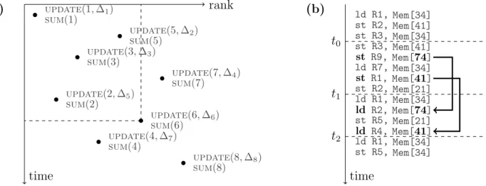
3.2 Information Transfer . . . 48
3.3 Interleaves . . . 49
3.4 A Tree For The Lower Bound . . . 50
3.5 The Bit-Reversal Permutation . . . 52
3.6 Dynamic Connectivity: The Hard Instance . . . 53
3.7 The Main Trick: Nondeterminism . . . 55
3.8 Proof of the Nondeterministic Bound . . . 55
3.9 Bibliographical Notes . . . 58
4 Epoch-Based Lower Bounds 59 4.1 Trade-offs and Higher Word Sizes . . . 60
4.2 Bit-Probe Complexity . . . 60
4.3 Lower Bounds for Partial Sums . . . 63
4.3.1 Formal Framework . . . 64
4.3.2 Bounding Probes into an Epoch . . . 65
4.3.3 Deriving the Trade-offs of Theorem 4.1 . . . 67
4.3.4 Proof of Lemma 4.3 . . . 68
5 Communication Complexity 71 5.1 Definitions . . . 71
5.1.1 Set Disjointness . . . 71
5.1.2 Complexity Measures . . . 72
5.2 Richness Lower Bounds . . . 72
5.2.1 Rectangles . . . 73
5.2.2 Richness . . . 74
5.2.3 Application to Indexing . . . 74
5.3 Direct Sum for Richness . . . 75
5.3.1 A Direct Sum of Indexing Problems . . . 75
5.3.2 Proof of Theorem 5.6 . . . 76
5.4 Randomized Lower Bounds . . . 77
5.4.1 Warm-Up . . . 77
5.4.2 A Strong Lower Bound . . . 79
5.4.3 Direct Sum for Randomized Richness . . . 80
5.4.4 Proof of Lemma 5.17 . . . 82
6 Static Lower Bounds 85
6.1 Partial Match . . . 86
6.2 Approximate Near Neighbor . . . 87
6.3 Decision Trees . . . 89
6.4 Near-Linear Space . . . 90
7 Range Query Problems 93 7.1 The Butterfly Effect . . . 94
7.1.1 Reachability Oracles to Stabbing . . . 94
7.1.2 The Structure of Dynamic Problems . . . 95
7.2 Adding Structure to Set Disjointness . . . 98
7.2.1 Randomized Bounds . . . 99
7.3 Set Disjointness to Reachability Oracles . . . 99
8 Near Neighbor Search in `∞ 103 8.1 Review of Indyk’s Upper Bound . . . 104
8.2 Lower Bound . . . 107
8.3 An Isoperimetric Inequality . . . 109
8.4 Expansion in One Dimension . . . 110
9 Predecessor Search 113 9.1 Data Structures Using Linear Space . . . 115
9.1.1 Equivalence to Longest Common Prefix . . . 115
9.1.2 The Data Structure of van Emde Boas . . . 116
9.1.3 Fusion Trees . . . 117
9.2 Lower Bounds . . . 119
9.2.1 The Cell-Probe Elimination Lemma . . . 119
9.2.2 Setup for the Predecessor Problem . . . 120
9.2.3 Deriving the Trade-Offs . . . 121
9.3 Proof of Cell-Probe Elimination . . . 124
9.3.1 The Solution to the Direct Sum Problem . . . 125
Chapter 1
Introduction
1.1
What is the Cell-Probe Model?
Perhaps the best way to understand the cell-probe model is as the “von Neumann bottle-neck,” a term coined by John Backus in his 1977 Turing Award lecture. In the von Neumann architecture, which is pervasive in today’s computers, the memory and the CPU are isolated components of the computer, communicating through a simple interface. At sufficiently high level of abstraction, this interface allows just two functions: reading and writing the atoms of memory (be they words, cache lines, or pages). In Backus’ words, “programming is basically planning and detailing the enormous traffic of words through the von Neumann bottleneck.” Formally, let the memory be an array of cells, each having w bits. The data structure is allowed to occupy S consecutive cells of this memory, called “the space.” The queries, and, for dynamic data structures, the updates, are implemented through algorithms that read and write cells. The running time of an operation is just the number of cell probes, i.e. the number of reads and writes executed. All computation based on cells that have been read is free.
Formally, the cell-probe model is a “non-uniform” model of computation. For a static data structure the memory representation is an arbitrary function of the input database. The query and update algorithms may maintain unbounded state, which is reset between operations. The query/update algorithms start with a state that stores the parameters of the operation; any information about the data structure must be learned through cell probes. The query and updates algorithms are arbitrary functions that specify the next read and write based on the current state, and specify how the state changes when a value is read.
1.1.1
Examples
Let us now exemplify with two fundamental data structure problems that we want to study. In Chapter 2, we introduce a larger collection of problems that the thesis is preoccupied with.
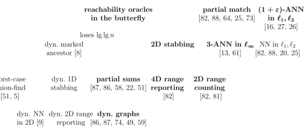
In the partial sums problem, the goal is to maintain an array A[1 . . n] of words (w-bit integers), initialized to zeroes, under the following operations:
update(k,∆): modify A[k]←∆.
sum(k): returns the partial sum Pki=1A[i].
The following are three very simple solutions to the problem:
• store that array A in plain form. The update requires 1 cell probe (update the corresponding value), while the query requires up to n cell probes to add values
A[1] +· · ·+A[k].
• maintain an array S[1 . . n], where S[k] = Pk
i=1A[i]. The update requires O(n) cell
probes to recompute all sums, while the query runs in constant time.
• maintain an augmented binary search tree with the array element in the leaves, where each internal node stores the sum of the leaves in its subtree. Both the query time and the update time areO(logn).
Dynamic problems are characterized by a trade-off between the update time tu and the
query time tq. Our goal is to establish the optimal trade-off, by describing a data structure
and a proof of a matching lower bound.
In most discussion in the literature, one is interested in the “running time per operation”, i.e. a single value max{tu, tq}which describes the complexity of both operations. In this view,
we will say that the partial sums problem admits an upper bound of O(lgn), and we will seek an Ω(lgn) lower bound. Effectively, we want to prove that binary search trees are the optimal solution for this problem.
To give an example of a static problem, consider predecessor search. The goal is to preprocess a setA ofn integers (of wbits each), and answer the following query efficiently:
predecessor(x): find max{y∈A|y < A}.
This problem can be solved with space O(n), and query time O(lgn): simply store the array in sorted order, and solve the query by binary search. Static problems can always be solved by complete tabulation: storing the answers to all possible queries. For predecessor search, this gives space O(2w), and constant query time. Later, we will see better upper bounds for this problem.
Static problems are characterized by a trade-off between the space S and the query time
t, which we want to understand via matching upper and lower bounds. In the literature, one is often interested in the query time achievable with linear, or near-linear space S =
O(npolylogn).
1.1.2
Predictive Power
For maximal portability, upper bounds for data structures are often designed in the word RAM model of computation, which considers any operation from the C programming lan-guage as “constant time.” Sometimes, however, it makes sense to consider variations of the model to allow a closer alignment of the theoretical prediction and practical performance. For example, one might augment the model with a new operation available on a family of CPUs. Alternatively, some operations, like division or multiplication, may be too slow on a
time epoch: # updates: # bits written: u 0 r0 tuw u u 1 r1 rtuw u u u u 2 r2 r2t uw u u u u u u u u 3 r3 r3t uw u u u u u u u u u u u u u u u u 4 r4 r4t uw ? query
info about epoch 3: 0 (r0+r1+r2)t
uw <2r2tuwbits Figure 1-1: Epochs grow exponentially at a rate of r, looking back from the query. Not enough information about epoch 3 is recorded outside it, so the query needs to probe a cell from epoch 3 with constant probability.
particular CPU, and one may exclude them from the set of constant-time operations while designing a new data structure.
By contrast, it has been accepted for at least two decades that the “holy grail” of lower bounds is to show results in the cell-probe model. Since the model ignores details particular to the CPU (which operations are available in the instruction set), a lower bound will apply to any computer that fits the von Neumann model. Furthermore, the lower bound holds for any implementation in a high-level programming language (such asC), since these languages enforce a separation between memory and the processing unit.
To obtain realistic lower bounds, it is standard to assume that the cells have w= Ω(lgn) bits. This allows pointers and indices to be manipulated in constant time, as is the case on modern computers and programming languages. To model external memory (or CPU caches), one can simply let w≈Blgn, where B is the size of a page or cache line.
1.2
Overview of Cell-Probe Lower Bounds
The cell-probe model was introduced three decades ago, by Yao [106] in FOCS’78. Unfor-tunately, his initial lower bounds were not particularly strong, and, as it often happens in Computer Science, the field had to wait for a second compelling paper before it took off.
In the case of cell-probe complexity, this came not as a second paper, but as a pair of almost simultaneous papers appearing two decades ago. In 1988, Ajtai [3] proved a lower bound for a static problem: predecessor search. In STOC’89, Fredman and Saks [51] proved the first lower bounds for dynamic problems, specifically for the partial sums problem and for union-find.
Static and dynamic lower bounds continued as two largely independent threads of re-search, with the sets of authors working on the two fields being almost disjoint. Dynamic lower bounds relied on the ad hoc chronogram technique of Fredman and Saks, while static lower bounds were based on communication complexity, a well-studied field of complexity theory.
1.2.1
Dynamic Bounds
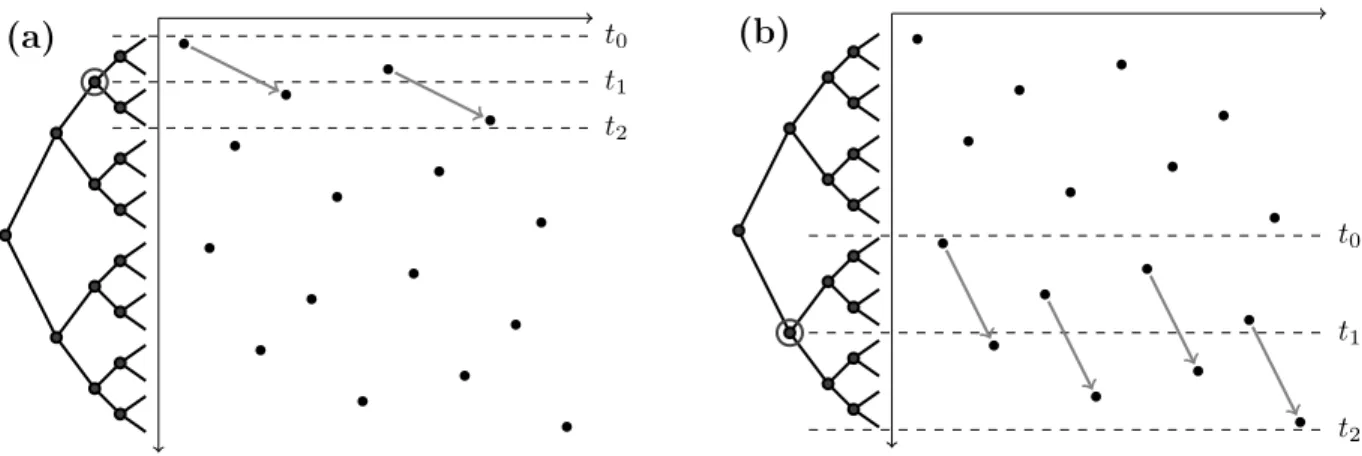
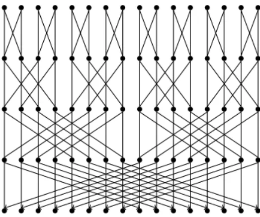
We first sketch the idea behind the technique of Fredman and Saks [51]; see Figure 1-1. The proof begins by generating a sequence of random updates, ended by exactly one query. Looking back in time from the query, we partition the updates into exponentially growing epochs: for a certain r, epoch i contains the ri updates immediately before epoch i−1.
The goal is to prove that for each i, the query needs to read a cell written in epoch i with constant probability. Then, by linearity of expectation over all epochs, we can bound the expected query time totq = Ω(logrn).
Observe that information about epoch i cannot be reflected in earlier epochs (those occurred back in time). On the other hand, the latest i−1 epochs contain less than 2·ri−1
updates. Assume the cell-probe complexity of each update is bounded by tu. Then, during
the latest i−1 epochs, only 2ri−1t
uw bits are written. Setting r=C·tuw for a sufficiently
large constant C, we have ri 2ri−1t
uw, so less than one bit of information is reported
about each update in epoch i. Assume that, in the particular computation problem that we want to lower bound, a random query is forced to learn information about a random update from each epoch. Then, the query must read a cell from epoch i with constant probability, because complete information about the needed update is not available outside the epoch. We have a lower bound oftq = Ω(logrn) = Ω(lgn/lg(wtu)). For the natural case
w= Θ(lgn), we have max{tu, tq}= Ω(lgn/lg lgn).
All subsequent papers [22, 70, 74, 59, 8, 49, 5, 9, 58] on dynamic lower bounds used this epoch-based approach of Fredman and Saks (sometimes called the “chronogram technique”). Perhaps the most influential in this line of research was that the paper by Alstrup, Husfeldt, and Rauhe [8] from FOCS’98. They proved a bound for the so-called marked ancestor problem, and showed many reductions from this single bound to various interesting data-structure problems.
In STOC’99, Alstrup, Ben-Amram, and Rauhe [5] showed optimal trade-offs for the union-find problem, improving on the original bound of Fredman and Saks [51].
1.2.2
Round Elimination
The seminal paper of Ajtai [3] turned out to have a bug invalidating the results, though this did not stop it from being one of the most influential papers in the field. In STOC’94, Miltersen [71] corrected Ajtai’s error, and derived a new set of results for the predecessor problem. More importantly, he recasted the proof as a lower bound for asymmetric commu-nication complexity.
The idea here is to consider a communication game in which Alice holds a query and Bob holds a database. The goal of the players is to answer the query on the database, through communication. A cell-probe algorithm immediately gives a communication protocol: in each round, Alice sends lgS bits (an address), and Bob replies with w bits (the contents of the memory location). Thus, a lower bound on the communication complexity implies a lower bound on the cell-probe complexity.
and Miltersen [71], was made explicit in STOC’95 by Miltersen, Nisan, Safra, and Wigder-son [73]. This technique is based on theround elimination lemma, a result that shows how to eliminate a message in the communication protocol, at the cost of reducing the problem size. If all messages can be eliminated and the final problem size is nontrivial (superconstant), the protocol cannot be correct.
Further work on the predecessor problem included the PhD thesis of Bing Xiao [105], the paper of Beame and Fich from STOC’99 [21], and the paper of Sen and Venkatesh [95]. These authors obtained better lower bounds for predecessor search, by showing tighter versions of round elimination.
Another application of round elimination was described by Chakrabarti, Chazelle, Gum, and Lvov [26] in STOC’99. They considered thed-dimensional approximate nearest neighbor problem, with constant approximation and polynomial space, and proved a time lower bound of Ω(lg lgd/lg lg lgd). This initial bound was deterministic, but Chakrabarti and Regev [27] proved a randomized bound via a new variation of the round elimination lemma.
1.2.3
Richness
Besides explicitly defining the round elimination concept, Miltersen et al. [73] also introduced a second technique for proving asymmetric lower bounds for communication complexity. This technique, called the richness method, could prove bounds of the form: either Alice communicatesabits, or Bob communicatesbbits (in total over all messages). By converting a data structure with cell-probe complexity t into a communication protocol, Alice will communicate tlgS bits, and Bob will communicate t·w bits. Thus, we obtain the lower bound t ≥ min{ a
lgS, b
w}. Typically, the b values in such proofs are extremely large, and the
minimum is given by the first term. Thus, the lower bound is t ≥ a/lgS, or equivalently
S ≥2a/t.
The richness method is usually used for “hard” problems, like nearest neighbor in high dimensions, where we want to show a large (superpolynomial) lower bound on the space. The bounds we can prove, having form S ≥ 2a/t, are usually very interesting for constant
query time, but they degrade very quickly with largert.
The problems that were analyzed via the richness method were:
• partial match (searching with wildcards), by Borodin, Ostrovsky, and Rabani [25] in STOC’99, and by Jayram, Khot, Kumar, and Rabani [64] in STOC’03.
• exact near neighbor search, by Barkol and Rabani [20] in STOC’00. Note that there exists a reduction from partial match to exact near neighbor. However, the bounds for partial match were not optimal, and Barkol and Rabani chose to attack near neighbor directly.
1.3
Our Contributions
In our work, we attack all the fronts of cell-probe lower bounds described above.
1.3.1
The Epoch Barrier in Dynamic Lower Bounds
As the natural applications of the chronogram technique were being exhausted, the main bar-rier in dynamic lower bounds became the chronogram technique itself. By design, the epochs have to grow at a rate of at least Ω(tu), which means that the large trade-off that can be
shown istq= Ω(lgn/lgtu), making the largest possible bound max{tu, tq}= Ω(lgn/lg lgn).
This creates a rather unfortunate gap in our understanding, since upper bounds ofO(lgn) are in abundance: such bounds are obtained via binary search trees, which are probably the single most useful idea in dynamic data structures. For example, the well-studied partial sums problem had an Ω(lgn/lg lgn) lower bound from the initial paper of Fredman and Saks [51], and this bound could not be improved to show that binary search trees are optimal. In 1999, Miltersen [72] surveyed the field of cell-probe complexity, and proposed sev-eral challenges for future research. Two of his three “big challenges” asked to prove an
ω(lgn/lg lgn) lower bound for any dynamic problem in the cell-probe model, respectively anω(lgn) lower bound for any problem in the bit-probe model (see§1.3.2). Of the remaining four challenges, one asked to prove Ω(lgn) for partial sums.
These three challenges are solved in our work, and this thesis. In joint work with Erik Demaine appearing in SODA’04 [84], we introduced a new technique for dynamic lower bounds, which could prove an Ω(lgn) lower bound for the partial sums problem. Though this was an important 15-year old open problem, the solution turned out to be extremely clean. The entire proof is some 3 pages of text, and includes essentially no calculation.
In STOC’04 [83], we augmented our technique through some new ideas, and obtained Ω(lgn) lower bounds for more problems, including an instance of list manipulation, dynamic connectivity, and dynamic trees. These two publications were merged into a single journal paper [86].
The logarithmic lower bounds are described in Chapter 3. These may constitute the easiest example of a data-structural lower bound, and can be presented to a large audience. Indeed, our proof has been taught in a course by Jeff Erickson at the University of Illinois at Urbana and Champaign, and in a course co-designed by myself and Erik Demaine at MIT.
1.3.2
The Logarithmic Barrier in Bit-Probe Complexity
The bit-probe model of computation is an instantiation of the cell-probe model with cells of
w = 1 bit. While this lacks the realism of the cell-probe model with w = Ω(lgn) bits per cell, it is a clean theoretical model that has been studied often.
In this model, the best dynamic lower bound was Ω(lgn), shown by Miltersen [74]. In his survey of cell-probe complexity [72], Miltersen lists obtaining anω(lgn) bound as one of the three “big challenges” for future research.
We address this challenge in our joint work with Tarnit¸ˇa [87] appearing in ICALP’05. Our proof is based on a surprising discovery: we present a subtle improvement to the classic chronogram technique of Fredman and Saks [51], which, in particular, allows it to prove logarithmic lower bounds in the cell-probe model. Given that the chronogram technique was the only known approach for dynamic lower bounds before our work in 2004, it is surprising to find that the solution to the desired logarithmic bound has always been this close.
To summarize our idea, remember that in the old epoch argument, the information revealed by epochs 1, . . . , i−1 about epochi was bounded by the number of cells written in these epochs. We will now switch to a simple alternative bound: the number of cells read during epochs 1, . . . , i−1 and written during epochi. This doesn’t immediately help, since all cell reads from epochi−1 could read data from epochi, making these two bounds identical. However, one can randomize the epoch construction, by inserting the query after a random
number of updates. This randomization “smoothes” out the distribution of epochs from which cells are read, i.e. a query readsO(tq/logrn) cells from every epoch, in expectation over
the randomness in the epoch construction. Then, theO(ri−1) updates in epochs 1, . . . , i−1
only read O(ri−1 ·t
u/logrn) cells from epoch i. This is not enough information if r
tu/logrn = Θ(tu/tq), which implies tq = Ω(logrn) = Ω(lgn/lgttuq). From this, it follows
that max{tu, tq}= Ω(lgn).
Our improved epoch technique has an immediate advantage: it is the first technique that can prove a bound for the regime tu < tq. In particular, we obtain a tight update/query
trade-off for the partial sums problem, whereas previous approaches could only attack the case tu > tq. Furthermore, by carefully using the new lower bound in the regime tu < tq,
we obtain an Ω (lg lglgnn)2 lower bound in the bit-prove model. This offers the highest known bound in the bit-probe model, and answers Miltersen’s challenge.
Intuitively, performance in the bit-probe model should typically be slower by a lgn factor compared to the cell-probe model. However, our Ω(lge 2n) bound in the bit-probe world is
far from an echo of anΩ(lge n) bound in the cell-probe world. Indeed, Ω(lg lglgnn) bounds in the
cell-probe model have been known since 1989, but the bit-probe record has remained just the slightly higher Ω(lgn). In fact, our bound is the first to show a quasi-optimal Ω(lge n)
separation between bit-probe complexity and the cell-probe complexity, for superconstant cell-probe complexity.
Our improved epoch construction, as well as our bit-probe lower bounds, are presented in Chapter 4.
1.3.3
The Communication Barrier in Static Complexity
All bounds for static data structures were shown by transforming the cell-probe algorithm into a communication protocol, and proving a communication lower bound for the problem at hand, either by round elimination, or by the richness method.
Intuitively, we do not expect this relation between cell-probe and communication com-plexity to be tight. In the communication model, Bob can remember past communication, and may answer new queries based on this. Needless to say, if Bob is just a table of cells, he
cannot “remember” anything, and his responses must be a function of Alice’s last message (i.e. the address being probed).
The most serious consequence of the reduction to communication complexity is that the lower bounds are insensitive to polynomial changes in the space S. For instance, going from space S =O(n3) to spaceS =O(n) only translates into a change in Alice’s message size by
a factor of 3. In the communication game model, this will increase the number of rounds by at most 3, since Alice can break a longer message into three separate messages, and Bob can remember the intermediate parts.
Unfortunately, this means that communication complexity cannot be used to separate data structures of polynomial space, versus data structures of linear space. By contrast, for many natural data-structure problems, the most interesting behavior occurs close to linear space. In fact, when we consider applications to large data bases, the difference between space O(n3) and space O(npolylogn) is essentially the difference between interesting and uninteresting solutions.
In our joint work with Mikkel Thorup [89] appearing in STOC’06, we provided the first separation between data structures of polynomial size, and data structures of linear size. In fact, our technique could prove an asymptotic separation between space Θ(n1+ε) and space
n1+o(1), for any constantε >0.
Our idea was to consider a communication game in which Alice holds k independent queries to the same database, for large k. At each step of the cell-probe algorithm, these queries need to probe a subset of at most k cells from the space of S cells. Thus, Alice needs to send O(lg Sk) = O(klgSk) bits to describe the memory addresses. For k close to n, and S = n1+o(1), this is asymptotically smaller than klgS. This means that the “amortized” complexity per query is o(lgS), and, if our lower bound per query is as high as for a single query, we obtain a better cell-probe lower bound. A result in communication complexity showing that the complexity of k independent problems increases by a factor of Ω(k) compared to one problem is called a direct sum result.
In our paper [89], we showed a direct sum result for the round elimination lemma. This implied an optimal lower bound for predecessor search, finally closing this well-studied prob-lem. Since predecessor search admits better upper bounds with spaceO(n2) than with space O(npolylogn), a tight bound could not have been obtained prior to our technique breaking the communication barrier.
For our direct sum version of round elimination, and our improved predecessor bounds, the reader is referred to Chapter 9.
1.3.4
Richness Lower Bounds
A systematic improvement. A broad impact of our work on the richness method was to show that the cell-probe consequence of richness lower bounds had been systematically underestimated: any richness lower bound implies better cell-probe lower bounds than what was previously thought, when the space is n1+o(1). In other words, we can take any lower
bound shown by the richness method, and obtain a better lower bound for small-space data structures by black-box use of the old result.
Remember that proving Alice must communicate Ω(a) bits essentially implies a cell-probe lower bound of t = Ω(a/lgS). By our trick for beating communication complexity, we will consider k = O(n/poly(w)) queries in parallel, which means that Alice will communicate
O(t·klgS
k) =O(tklg Sw
n ) bits in total.
Our novel technical result is a direct sum theorem for the richness measure: for any problemf that has an Ω(a) communication lower bound by richness,kindependent copies of
f will have a lower bound of Ω(k·a). This implies thatt·klgSwn = Ω(k·a), sot= Ω(a/lgSwn ). Our new bounds is better than the classict = Ω(a/lgS), for space n1+o(1). In particular, for
the most important case of S =O(npolylogn) and w=O(polylogn), our improved bound is better by Θ(lgn/lg lgn).
Our direct sums theorems for richness appeared in joint work with Mikkel Thorup [88] at FOCS’06, and are described in Chapter 5.
Specific problems. Our work has also extended the reach of the richness method, proving lower bound for several interesting problem.
One such problem is lopsided set disjointness (LSD), in which Alice and Bob receive
sets S and T (|S| |T|), and they want to determine whether S ∩ T = ∅. In their seminal work from STOC’95, Miltersen et al. [73] proved a deterministic lower bound for lopsided set disjointness, and left the randomized case as an “interesting open problem.” The first randomized bounds were provided in our joint work with Alexandr Andoni and Piotr Indyk [16], appearing in FOCS’06, and strengthened in our (single-author) paper [82] appearing in FOCS’08. Some of these lower bounds are described in Chapter 5.
Traditionally,LSDwas studied for its fundamental appeal, not because of data-structural
applications. However, in [82] we showed a simple reduction from LSD to partial match.
Despite the work of [73, 25, 64], the best bound for partial match was suboptimal, showing that Alice must communicate Ω(d/lgn) bits, where d is the dimension. Our reduction, coupled with our LSD result, imply an optimal bound of Ω(d) on Alice’s communication,
closing this issue. The proof of our reduction appears in Chapter 6.
Since partial match reduces to exact near neighbor, we also obtain an optimal communi-cation bound for that problem. This supersedes the work of [20], who had a more complicated proof of a tight lower bound for exact near neighbor.
Turning our attention to (1 +ε)-approximate nearest neighbor, we find the existing lower bounds unsatisfactory. The upper bounds for this problem use nO(1/ε2)
space, by dimension-ality reduction. On the other hand, the lower bounds of [26, 27] allowed constant ε and polynomial space, proving a tight time lower bound of Ω(lg lgd/lg lg lgd) in d dimensions. However, from a practical perspective, the main issue with the upper bound is the prohibitive space usage, not the doubly logarithmic query time. To address this concern, our paper with Andoni and Indyk [16] proved a communication lower bound in which Alice’s communication is Ω(ε12 lgn) bits. This shows that the space must be nΩ(1/(tε
2))
, for query time t. Our lower bound is once more by reduction from LSD, and can be found in Chapter 6.
Finally, we consider the near neighbor problem in the `∞ metric, in which Indyk [61] had shown an exotic trade-off between approximation and space, obtaining O(lg lgd)
approxi-mation for any polynomial space. In our joint work with Andoni and Croitoru [13], we gave a very appealing reformulation of Indyk’s algorithm in information-theoretic terms, which made his space/approximation trade-off more natural. Then, we described a richness lower bound for the problem, showing that this space/approximation trade-off is optimal. These results can be found in Chapter 8.
1.3.5
Lower Bounds for Range Queries
By far, the most exciting consequence of our technique for surpassing the communication barrier is that it opens the door to tight bounds for range queries. Such queries are some of the most natural examples of what computers might be queried for, and any statement about their importance is probably superfluous. The introductory lecture of any database course is virtually certain to contain an example like “find employees with a salary between 70000 and 95000, who have been hired between 1998 and 2001.”
Orthogonal range queries can be solved in constant time if polynomial space is allowed, by simply precomputing all answers. Thus, any understanding of these problems hinges on our technique to obtain better lower bounds for space O(npolylogn).
In my papers [81, 82], I prove optimal bounds for range counting in 2 dimensions, stabbing in 2 dimensions, and range reporting in 4 dimensions. Surprisingly, our lower bounds are once more by reduction from LSD.
Range counting problems have traditionally been studied in algebraic models. In the group and semigroup models, each point has an associated weight from an arbitrary commu-tative (semi)group and the “counting” query asks for the sum of the weights of the points in the range. The data structure can only manipulate weights through the black-box addition operator (and, in the group model, subtraction).
The semigroup model has allowed for every strong lower bounds, and nearly optimal results are known in all dimensions. By contrast, as soon as we allow subtraction (the group model), the lower bounds are very weak, and we did not even have a good bound for 2 dimensions. This rift between our understanding of the semigroup and stronger models has a deeper conceptual explanation. In general, semigroup lower bounds hide arguments of a very geometric flavor. If a value is included in a sum, it can never be taken out again (no subtraction is available), and this immediately places a geometric restriction on the set of ranges that could use the cell. Thus, semigroup lower bounds are essentially bounds on a certain kind of “decomposability” of geometric shapes. On the other hand, bounds in the group or cell-probe model require a different, information theoretic understanding of the problem. In the group model, the sum stored in a cell does not tell us anything in isolation, as terms could easily be subtracted out. The lower bound must now find certain bottlenecks in the manipulation of information that make the problem hard. Essentially, the difference in the type of reasoning behind semigroup lower bounds and group/cell-probe lower bounds is parallel to the difference between “understanding geometry” and “understanding computation”. Since we have been vastly more successful at the former, it should not come as a surprise that progress outside the semigroup model has been extremely slow.
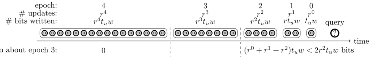
lopsided set disjointness[82, 16, 73] reachability oracles in the butterfly loses lg lgn partial match [82, 88, 64, 25, 73] (1 +ε)-ANN in `1, `2 [16, 27, 26] dyn. marked ancestor [8] 2D stabbing 3-ANN in`∞ [13, 61] NN in `1, `2 [82, 88, 20, 25] worst-case union-find [51, 5] dyn. 1D stabbing partial sums [87, 86, 58, 22, 51] 4D range reporting [82] 2D range counting [82, 81] dyn. NN in 2D [9] dyn. 2D range reporting dyn. graphs [86, 87, 74, 49, 59]
Figure 1-2: Dashed lines indicate reductions that were already known, while solid lines indicate novel reductions. For problems in bold, the results of this thesis are stronger than what was previously known. Citations indicate work on lower bounds.
an important challenge. As early as 1982, Fredman [48] asked for better bounds in the group model for dynamic range counting. In FOCS’86, Chazelle [31] echoed this, and also asked about the static case. Our results answer these old challenges, at least in the 2-dimensional case.
1.3.6
Simple Proofs
An important contribution of our work is to show clean, simple proofs of lower bounds, in an area of Theoretical Computer Science that is often dominated by exhausting technical details.
Perhaps the best illustration of this contribution is in Figure 1-2, which shows the lower bounds that can be obtained by reduction from lopsided set disjointness. (The reader unfa-miliar with the problems can consult Chapter 2.)
This reduction tree is able to unify a large fraction of the known results in dynamic data structures and static data structures (both in the case of large space, and for near-linear space). In many cases, our proofs by reduction considerably simplify the previous proofs. Putting all the work in a single lower bound has exciting consequences from the teaching perspective: instead of presenting many different lower bounds (even “simple” ones are seldom light on technical detail!), we can now present many interesting results through clean algorithmic reductions, which are easier to grasp.
Looking at the reduction tree, it may seem hard to imagine a formal connection between lower bounds for such different problems, in such different settings. Much of the magic of our results lies in considering a somewhat artificial problem, which nonetheless gives the right
link between the problems: reachability queries in butterfly graphs. Once we decide to use this middle ground, it is not hard to give reductions to and from set disjointness, dynamic marked ancestor, and static 4-dimensional range reporting. Each of these reductions is natural, but the combination is no less surprising.
Chapter 2
Catalog of Problems
This section introduces the various data-structure problems that we consider throughout this thesis. It is hoped that the discussion of each topic is sufficiently self-contained, that the reader can quickly jump to his or her topic of interest.
2.1
Predecessor Search
2.1.1
Flavors of Integer Search
Binary search is certainly one of the most fundamental ideas in computer science — but what do we use it for? Given a setS with |S|=n values from some ordered universeU, the following are natural and often-asked queries the can be solved by binary search:
exact search: given some x∈U, isx∈S?
predecessor search: given some x∈U, find max{y ∈S |y < S}, i.e. the predecessor of
x in the set S.
1D range reporting: given some interval [x, y], report all/one of the points in S∩[x, y]. Exact search is ubiquitous in computer science, while range reporting is a natural and important database query. Though at first sight predecessor search may seem less natural, it may in fact be the most widely used of the three. Some of its many applications include:
• IP-lookup, perhaps the most important application, is the basic query that must be answered by every Internet router when forwarding a packet (which probably makes it the most executed algorithmic problem in the world). The problem is equivalent to predecessor search [44].
• to make data structures persistent, each cell is replaced with a list of updates. Deciding which version to use is a predecessor problem.
• orthogonal range queries start by converting any universeU into “rank space”{1, . . . , n}. The dependence on the universe becomes an additive term in the running time.
• the succinct incarnation of predecessor search is known as the “rank/select problem,” and it underlies most succinct data structures.
• (1 +ε)-approximate near neighbor in any constant dimension (with the normal Eu-clidean metric) is equivalent to predecessor search [28].
• in the emergency planning version of dynamic connectivity, a query is equivalent to predecessor search; see our work with Mikkel Thorup [85].
It is possible to study search problems in an arbitrary universe U endowed with a com-parison operation (the so called comparison model), in which case the Θ(lgn) running time of binary search is easily seen to be optimal. However, this “optimality” of binary search is misleading, given that actual computers represent data in some well-specified formats with bounded precision.
The most natural universe is U ={0, . . . ,2w−1}, capturing the assumption that values
are arbitrary w-bit integers that fit in a machine word. The standard floating point repre-sentation (IEEE 754, 1985) was designed so that twow-bit floating point values compare the same as two w-bit integers. Thus, any algorithm for search queries that applies to integers carries over to floating point numbers. Furthermore, most algorithms apply naturally to strings, which can be interpreted as numbers of high, variable precision.
By far, the best known use of bounded precision is hashing. In fact, when one thinks of exact search queries, the first solution that comes to mind is probably hash tables, not binary search. Hash tables provide an optimal solution to this problem, at least if we accept randomization in the construction. Consider the following theorem due to Fredman, Koml´os, and Szemer´edi [50]:
Theorem 2.1. There exists a dictionary data structure using O(n) words of memory that answers exact search queries deterministically in O(1) time. The data structure can be constructed by a randomized algorithm in O(n) time with high probability.
Dietzfelbinger and Meyer auf der Heide [39] give a dynamic dictionary that implements queries deterministically in constant time, while the randomized updates run in constant time with high probability.
By contrast, constant time is not possible for predecessor search. The problem has been studied intensely in the past 20 years, and it was only in our recent work with Mikkel Thorup [89, 90] that the optimal bounds were understood. We discuss the history of this problem in the next section.
One-dimensional range reporting remains the least understood of the three problems. In our work with Christian Mortensen and Rasmus Pagh [76], we have shown surprising upper bounds for dynamic range reporting in one dimension, with a query time that is exponentially faster than the optimal query time for predecessor search. However, there is currently no lower bound for the problem, and we do not know whether it requires superconstant time per operation.
2.1.2
Previous Upper Bounds
The famous data structure of van Emde Boas [101] from FOCS’75 can solve predecessor search in O(lgw) = O(lg lgU) time, using linear space [103]. The main idea of this data
structure is to binary search for the longest common prefix between the query and a value in the database.
It is interesting to note that the solution of van Emde Boas remains very relevant in modern times. IP look-up has received considerable attention in the networking community, since a very fast solution is needed for the router to keep up with the connection speed. Research [44, 36, 102, 1] on software implementations of IP look-up has rediscovered the van Emde Boas solution, and engineered it into very efficient practical solutions.
In external memory with pages of B words, predecessor search can be solved by B-trees in time O(logBn). In STOC’90, Fredman and Willard [52] introduced fusion trees, which use an ingenious packing of multiple values into a single word to simulate a page of size
B = wε. Fusion trees solve predecessor search in linear space and O(log
wn) query time.
Since w = Ω(lgn), the search time is always O(lgn/lg lgn), i.e. fusion trees are always asymptotically better than binary search. In fact, taking the best of fusion trees and van Emde Boas yields a search time ofO(min{lglgwn, lgw})≤O(√lgn). Variations on fusion trees include [53, 104, 11, 10], though the O(logwn) query time is not improved.
In 1999, Beame and Fich [21] found a theoretical improvement to van Emde Boas’ data structure, bringing the search time down toO(lg lglgww). Combined with fusion trees, this gave them a bound of O(min{lglgwn, lg lglgww})≤ O(
q
lgn
lg lgn). Unfortunately, the new data structure
of Beame and Fich usesO(n2) space, and their main open problems asked whether the space could be improved to (near) linear.
The exponential trees of Andersson and Thorup [12] are an intriguing construction that uses a predecessor structure for nγ “splitters,” and recurses in each bucket of O(n1−γ)
el-ements found between pairs of splitters. Given any predecessor structure with polynomial space and query timetq≥lgεn, this idea can improve it in a black-box fashion to use O(n)
space and O(tq) query time. Unfortunately, applied to the construction of Beame and Fich,
exponential trees cannot reduce the space to linear without increasing the query to O(lgw). Nonetheless, exponential trees seem to have generated optimism that the van Emde Boas bound can be improved.
Our lower bounds, which are joint work with Mikkel Thorup [89, 90] and appear Chap-ter 9, refute this possibility and answer the question of Beame and Fich in the negative. We show that for near-linear space, such as spacen·lgO(1)n, the best running time is essentially the minimum of the two classic solutions: fusion trees and van Emde Boas.
2.1.3
Previous Lower Bounds
Ajtai [3] was the first to prove a superconstant lower bound. His results, with a correction by Miltersen [71], show that for polynomial space, there exists n as a function of w making the query time Ω(√lgw), and likewise there exists w a function of n making the query complexity Ω(√3lgn).
Miltersen et al. [73] revisited Ajtai’s proof, extending it to randomized algorithms. More importantly, they captured the essence of the proof in an independent round elimination lemma, which is an important tool for proving lower bounds in asymmetric communication.
Beame and Fich [21] improved Ajtai’s lower bounds to Ω(lg lglgww) and Ω(qlg lglgnn) respec-tively. Sen and Venkatesh [95] later gave an improved round elimination lemma, which extended the lower bounds of Beame and Fich to randomized algorithms.
Chakrabarti and Regev [27] introduced an alternative to round elimination, the message compression lemma. As we showed in [89], this lemma can be used to derive an optimal space/time trade-off when the space is S ≥n1+ε. In this case, the optimal query time turns out to be Θ min
logwn,lg lglgwS .
Our result seems to have gone against the standard thinking in the community. Sen and Venkatesh [95] asked whether message compression is really needed for the result of Chakrabarti and Regev [27], or it could be replaced by standard round elimination. By contrast, our result shows that message compression is essential even for classic predecessor lower bounds.
It is interesting to note that the lower bounds for predecessor search hold, by reductions, for all applications mentioned in the previous section. To facilitate these reductions, the lower bounds are in fact shown for the colored predecessor problem: the values in S are colored red or blue, and the query only needs to return the color of the predecessor.
2.1.4
Our Optimal Bounds
Our results from [89, 90] give an optimal trade-off between the query time and the spaceS. Letting a= lgSn·w, the query time is, up to constant factors:
min logwn lgw−algn lgw a lg(lgan·lgwa) lgwa lg(lgwa /lglgan) (2.1)
The upper bounds are achieved by a deterministic query algorithm. For any space S, the data structure can be constructed in timeO(S) with high probability, starting from a sorted list of integers. In addition, our data structure supports efficient dynamic updates: iftqis the
query time, the (randomized) update time is O(tq+Sn) with high probability. Thus, besides
locating the element through one predecessor query, updates change a minimal fraction of the data structure.
In the external memory model with pages of B words, an additional term of logBn is added to (2.1). Thus, our result shows that it is always optimal to either use the standard B-trees, or ignore external memory completely, and use the best word RAM strategy.
For space S =n·poly(wlgn) and w≥(1 +ε) lgn, the trade-off is simplified to: min logwn, lgwlg w
The first branch corresponds to fusion trees. The second branch demonstrates that van Emde Boas cannot be improved in general (for all word sizes), though a very small improvement can be made for word size w >(lgn)ω(1). This improvement is described in our paper with Mikkel Thorup [89].
Our optimal lower bound required a significant conceptual development in the field. Previously, all lower bounds were shown via communication complexity, which fundamentally cannot prove a separation between data structures of polynomial size and data structures of linear size (see Chapter 1). This separation is needed to understand predecessor search, since Beame and Fich beat the van Emde Boas bound using quadratic space.
The key idea is to analyze many queries simultaneously, and prove a direct-sum version of the round elimination lemma. As opposed to previous proofs, our results cannot afford to increase the distributional error probability. Thus, a second conceptual idea is to consider a stronger model for the induction on cell probes: in our model, the algorithm is allowed to
reject a large fraction of the queries before starting to make probes.
This thesis. Since this thesis focuses of lower bounds, we omit a discussion of the upper bounds. Furthermore, we want to avoid the calculations involved in deriving the entire trade-off of (2.1), and keep the thesis focused on the techniques. Thus, we will only prove the lower bound for the casew= Θ(lgn), which is enough to demonstrate the optimality of van Emde Boas, and a separation between linear and polynomial space. The reader interested in the details of the entire trade-off calculation is referred to our publication [89].
In Chapter 9, we first review fusion trees and the van Emde Boas data structure from an information-theoretic perspective, building intuition for our lower bound. Then, we prove our direct-sum round elimination for multiple queries, which implies the full trade-off (2.1) (though, we only include the calculation for w= 3 lgn).
2.2
Dynamic Problems
2.2.1
Maintaining Partial Sums
This problem, often described as “maintaining a dynamic histogram,” asks to maintain an array A[1 . . n] of integers, subject to:
update(k,∆): modify A[k]←∆, where ∆ is an arbitrary w-bit integer. sum(k): returns the “partial sum” Pki=1A[i].
This problem is a prototypical application of augmented binary search trees (BSTs), which give an O(lgn) upper bound. The idea is to consider a fixed balanced binary tree with n
leaves, which represent the n values of the array. Each internal node is augmented with a value equal to the sum of the values in its children (equivalently, the sum of all leaves in the node’s subtree).
A large body of work in lower bounds has been dedicated to understanding the partial sums problem, and in fact, it is by far the best studied dynamic problem. This should
not come as a surprise, since augmented BSTs are a fundamental technique in dynamic data structures, and the partial sums problem likely offers the cleanest setting in which this technique can be studied.
2.2.2
Previous Lower Bounds
The partial-sums problem has been a favorite target for new lower bound ideas since the dawn of data structures. Early efforts concentrated on algebraic models of computation. In the semigroup or group models, the elements of the array come from a black-box (semi)group. The algorithm can only manipulate the ∆ inputs through additions and, in the group model, subtractions; all other computations in terms of the indices touched by the operations are free.
In the semigroup model, Fredman [47] gave a tight Ω(lgn) bound. Since additive inverses do not exist in the semigroup model, an update A[i] ← ∆ invalidates all memory cells storing sums containing the old value of A[i]. If updates have the form A[i] ← A[i] + ∆, Yao [107] proved a lower bound of Ω(lgn/lg lgn). Finally, in FOCS’93, Hampapuram and Fredman [54] proved an Ω(lgn) lower bound for this version of the problem.
In the group model, a tight bound (including the lead constant) was given by Fredman [48] for the restricted class of “oblivious” algorithms, whose behavior can be described by matrix multiplication. In STOC’89, Fredman and Saks [51] gave an Ω(lgn/lg lgn) bound for the general case, which remained the best known before our work.
In fact, the results of Fredman and Saks [51] also contained the first dynamic lower bounds in the cell-probe model. Their lower bound trade-off between the update time tu
and query timetqstates thattq = Ω(lgn
lg(w+tu+ lgn)), which implies that max{tu, tq}=
Ω(lgn
lg(w+ lgn)).
In FOCS’91, Ben-Amram and Galil [22] reproved the lower bounds of Fredman and Saks in a more formalized framework, centered around the concepts of problem and output vari-ability. Using these ideas, they showed [23] Ω(lgn/lg lgn) lower bounds in more complicated algebraic models (allowing multiplication, etc).
Fredman and Henzinger [49] reproved the lower bounds of [51] for a more restricted version of partial sums, which allowed them to construct reductions to dynamic connectivity, dynamic planarity testing, and other graph problems. Husfeldt, Rauhe, Skyum [59] also explored variations of the lower bound allowing reduction to dynamic graph problems.
Husfeldt and Rauhe [58] gave the first technical improvement after [51], by proving that the lower bounds hold even for nondeterministic query algorithms. A stronger improvement was given in FOCS’98 by Alstrup, Husfeldt, and Rauhe [8], who prove thattqlgtu = Ω(lgn).
While this bound cannot improve max{tu, tq} = Ω(lgn/lg lgn), it at least implies tq =
Ω(lgn) when the update time is constant.
The partial sums problem has also been considered in the bit-probe model of computation, where each A[i] is a bit. Fredman [48] showed a bound of Ω(lgn/lg lgn) for this case. The highest bound forany dynamic problem in the bit-probe model was Ω(lgn), due to Miltersen et al. [74].
In 1999, Miltersen [72] surveyed the field of cell-probe complexity, and proposed sev-eral challenges for future research. Two of his three “big challenges” asked to prove an
ω(lgn/lg lgn) lower bound for any dynamic problem in the cell-probe model, respectively an ω(lgn) lower bound for any problem in the bit-probe model. Of the remaining four challenges, one asked to prove Ω(lgn) for partial sums, at least in the group model of com-putation.
2.2.3
Our Results
In our work with Erik Demaine [86, 87], we broke these barriers in cell-probe and bit-probe complexity, and showed optimal bounds for the partial sums problem.
In Chapter 3, we describe a very simple proof of an Ω(lgn) lower bound for partial sums, finally showing that the natural upper bound of binary search trees is optimal. The cleanness of this approach (the proof is roughly 3 pages of text, involving no calculation) stands in sharp contrast to the 15 years that the problem remained open.
In Chapter 4, we prove a versatile trade-off for partial sums, via a subtle variation to the classic chronogram technique of Fredman and Saks [51]. This trade-off is optimal in the cell-probe model, in particular reproving the Ω(lgn) lower bound. It is surprising to find that the answer to Miltersen’s big challenges consists of a small variation of what was already know.
Our trade-off also allows us to show an Ω(lgn/lg lg lgn) bound for partial sums in the bit-probe model, improving on Fredman’s 1982 result [48]. Finally, it allows us to show an Ω lg lglgnn2 lower bound in the bit-probe model, for dynamic connectivity. This gives a new record for lower bounds in the bit-probe model, addressing Miltersen’s challenge to show an
ω(lgn) bound.
Intuitively, performance in the bit-probe model should typically be slower by a lgn factor compared to the cell-probe model. However, our Ω(lge 2n) bound in the bit-probe world is
far from an echo of anΩ(lge n) bound in the cell-probe world. Indeed, Ω( lgn
lg lgn) bounds in the
cell-probe model have been known since 1989, but the bit-probe record has remained just the slightly higher Ω(lgn). In fact, our bound is the first to show a quasi-optimal Ω(lge n)
separation between bit-probe complexity and the cell-probe complexity, for superconstant cell-probe complexity.
2.2.4
Related Problems
List manipulation. In practice, one often seeks a cross between linked lists and array: maintaing a collection of items under typical linked-list operations, with the additional in-dexing operation (that is typical of array). We can consider the following natural operations, ignoring all details of what constitutes a “record” (all manipulation is done through pointers to black-box records):
insert(p, r): insert recordr immediately after record pin its list. delete(r): delete record r from its list.
link(h1, h2): concatenate two lists, identified by their head records h1 and h2.
cut(h, p): split the list with head at h into two lists, the second beginning from record p. index(k, h): return a pointer to the k-th value in the list with header ath.
rank(p): return the rank (position) of record pin its list. find(p): return the head of the list that contains record p.
All these operations, and many variants thereof, can be solved in O(lgn) time per oper-ation using augmented binary search trees. For insert/delete updates, the binary search tree algorithm must be able to maintain balance in a dynamic tree. Such algorithms abound (consider red-black trees, AVL trees, splay trees, etc). For link/cut, the tree algorithm
must support split and merge operations. Many dynamic trees support these operations inO(lgn) time, including 2-3-4 trees, AVL trees, splay trees, etc.
It turns out that there is a complexity gap between list manipulation with link/cut
operations, and list manipulation with insert/delete. In the former case, updates can make large topological changes to the lists, while in the latter, the updates only have a very local record-wise effect.
If the set of operations includes link, cut, and any of the three queries (including the minimalist find), we can show an Ω(lgn) lower bound for list manipulation. Thus,
augmented binary search trees give an optimal solution. The lower bound is described in Chapter 3, and needs a few interesting ideas beyond the partial-sums lower bound.
If the set of updates is restricted to insert and delete (with all queries allowed),
the problem admits an O(lgn/lg lgn) solution, as proved by Dietz [38]. This restricted case of list manipulation can be shown equivalent to the partial sums problem, in which every array element is A[i] ∈ {0,1}. The original lower bound of Fredman and Saks [51], as well as our trade-off from Chapter 4 show a tight Ω(lgn/lg lgn) bound for restricted partial sums problem. By reduction, this implies a tight bound for list manipulation with
insert/delete.
Dynamic connectivity. Dynamic graph problems ask to maintain a graph under various operations (typically edge insertions and deletions), and queries for typical graph properties (connectivity of two vertices, MST, shortest path, etc). This has been a very active area of research in the past two decades, and many surprising results have appeared.
Dynamic connectivity is the most basic dynamic graph problem. It asks to maintain an undirected graph with a fixed set of n vertices subject to the following operations:
insert(u, v): insert an edge (u, v) into the graph. delete(u, v): delete the edge (u, v) from the graph.
connected(u, v): test whether u and v lie in the same connected component.
If the graph is always a forest, Sleator and Tarjan’s classic “dynamic trees” [97] achieve an
O(lgn) upper bound. A simpler solution is given by Euler tour trees [55], which show that the problem is equivalent to list manipulation. If we maintain the Euler tour of each tree as a list, then an insert or delete can be translated to O(1) link/cut operations, and the

![Figure 3-2: (a) The vertical lines describe the information that the queries in [t 1 , t 2 ] from the updates in [t 0 , t 1 ]](https://thumb-us.123doks.com/thumbv2/123dok_us/10314489.2940550/50.918.136.796.109.358/figure-vertical-lines-information-queries-t-t-updates.webp)