This paper can be downloaded without charge at: The Fondazione Eni Enrico Mattei Note di Lavoro Series Index: http://www.feem.it/Feem/Pub/Publications/WPapers/default.htm
Social Science Research Network Electronic Paper Collection: http://ssrn.com/abstract=1130159
The opinions expressed in this paper do not necessarily reflect the position of
Vertical Integration and
Operational Flexibility
Michele Moretto and Gianpaolo RossiniNOTA DI LAVORO 37.2008
APRIL 2008
ETA – Economic Theory and Applications
Michele Moretto, Department of Economics, University of Padova
Vertical Integration and Operational Flexibility
SummaryThe main aim of the paper is to highlight the relation between flexibility and vertical integration. To this purpose, we go through the selection of the optimal degree of vertical disintegration of a flexible firm which operates in a dynamic uncertain environment. The enterprise we model enjoys flexibility since it can switch from a certain amount of disintegration to vertical integration and viceversa. This means that the firm never loses vertical control, i.e., the ability to produce all inputs even when it buys them in the market. This sort of flexibility makes for results which are somehow contrary to the Industrial Organization recent literature and closer to the Operations Research results. In this sense we provide a bridge between the two approaches and rescue Industrial Organization from counterintuitive conclusions.
Keywords: Vertical Integration, Outsourcing, Entry, Flexibility JEL Classification: L24, G 31, C61
We wish to thank Laura Vici for the provision of vertical integration statistics. The paper will be presented at the 6th Annual IIOC at Marymount University Washington, DC, May 16-18, 2008. We acknowledge the financial support of the Universities of Bologna and Padova within the 2007-8 60% scheme.
Address for correspondence:
Michele Moretto
Department of Economics University of Padova Via del Santo 22 Padova
Italy
1
Introduction
A crucial question in both Industrial Organization and Operations Research concerns the extension of the control of a vertical production process and its flexibility. This topic has come recently to the limelight (Acemoglu, Aghion, Griffith and Zilibotti, 2005; Acemoglu, Johnson and Mitton, 2005; Rossini, 2005, 2007) following the current wave of international outsourcing (Antràs and Helpman, 2004; Grossman and Helpman, 2002, 2005) with many firms increasing vertical disintegration on a crossborder basis by buying a growing chunk of inputs from independent foreign enterprises.
Even though most of current outsourcing is due to lower labour costs in the countries where portions of the vertical process of production is off-shored, vertical disintegration is often chosen for reasons not directly linked to labour costs. As Grossman and Helpman (2002) pointed out, vertical dis-integration may allow finer specialization in input production due to scale economies in R&D and production. This effect may be amplified by trade deepening, owing to better opportunities to concentrate on fewer stages of production. Nonetheless, vertical disintegration may also be adopted as a cushion against external shocks. By sharing the vertical control of produc-tion with other, preferably foreign, enterprises, each firm may enjoy a more flexible and less risky production organization, especially whenever different stages of the vertical production process require bearing relevant sunk costs. On the contrary, high quality firms may decide to increase their degree of vertical integration to make sure that quality standards are more likely met. All these considerations are bound to explaini) why vertical disintegra-tion shows variable and opposite trends across time and industries, ii) why we observe outsourcing among similar countries and within the same coun-try, iii) why there are many examples of insourcing 1, i.e., increased vertical integration, for instance, as a result of vertical mergers2.
1In June 7, 2005 the president of the Confederation of Indian Industry (CII) Sunil
Bharti Mittal told Democratic presidential candidate Hillary Clinton about Indian com-panies outsourcing to US firms, investing in the US and creating jobs ( IANS, 2005). Moreover, in 2007 Glaxo-Smith-Kline has decided to bring back to Europe labs involved in advanced R&D located in China. Moreover, some increased insourcing has been noticed recently in some Japanese high tech firms and in some high quality - high tech US firms. These are just few examples of reverse outsourcing which can be found in newspapers and in specialized publications.
2In the food industry, in the automotive industry in emerging countries, such as Indian
So far the decision as to vertically disintegrate and/or integrate has been analyzed as a once and for all choice, i.e., without contemplating any oppor-tunity for its reversal. Yet, a question arises as to whether a firm may be better off adopting a radical vertical disintegration with the loss of control of entire phases of the production process (Helpman and Grossman, 2005) or it may be preferable to retain the ability to produce the inputs bought from independent enterprises. For instance, this may be obtained by producing in-house just a quota of the input requirement. As a matter of fact, for each level of external input procurement, there are many ways to vertically dis-integrate. When a firm decides to offshore an input production to a foreign independent firm, the associated risk (due to exchange rates, foreign rules, production conditions in a remote country, quality standards, delivery time, shipment costs, etc.) may be quite high and worth some prudential behavior. An industrial real (not financial) way to decrease, or diversify away, this risk may require either keeping a share of the process of production in-house as a buffer or simply preserving the ability (know how and some facilities) to make it and, perhaps, reverse the offshoring decision by bringing back sections of the vertical chain of production whenever circumstances dictate so.
All these considerations confirm that the decision to outsource is neither a simple binary choice, nor a matter of sheer input costs of production. Yet, it appears to be quite related to the extent of flexibility needed by a firm so as to safely face uncertainty.
Industrial Organization (Alvarez and Stenbacka, 2007) and Operations Research (Van Mieghen, 1999) offer different answers as to the optimal tim-ing and extent of outsourctim-ing vis à vis internal production. The Operations Research interpretation3 maintains that firms subcontract more as market uncertainty (risk) increases, closely paralleling the behavior of financial op-tions, whose worth increases with uncertainty.
In Industrial Organization literature, once the decision as to the verti-cal arrangement of a firm is taken there is no possibility of reversing it: the amount of flexibility that outsourcing is meant to provide cannot change once a certain vertical organization has been decided. Moreover, in Alvarez and
3Van Mieghem (1999) contribution belongs to Operations Research literature which
highlights the flexibility that subcontracting offers to production and capacity planning. Van Mieghem (1999) paper extends and generalizes previous studies (Li, 1992 and Mc-Cardle, 1997) which dealt only with the strategic unidimensional problem of optimal pro-duction with outsourcing, without considering capacity selection, i.e. the optimal size of investment.
Stenbacka (2007), at higher levels of uncertainty the adoption of outsourc-ing is beoutsourc-ing postponed. This result is actually puzzloutsourc-ing, contrary to both Van Mieghem (1999) and common sense, since, in an uncertain dynamic framework, outsourcing is a way to do "production and capacity smoothing" making for the presumption that higher uncertainty should accelerate the adoption of outsourcing. But in current Industrial Organization literature the firm has an option to do outsourcing, yet not to do "production (and profit) smoothing" by switching among different levels of vertical integration to minimize profit variability.
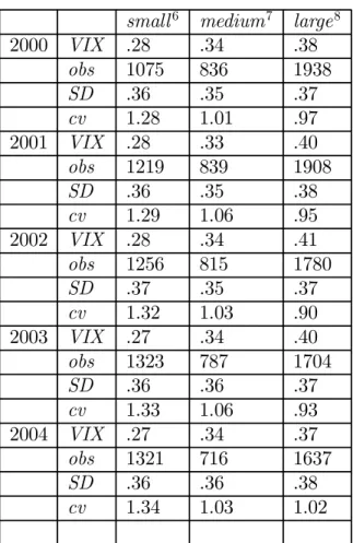
Recent literature (Acemoglu, Aghion, Griffith and Zilibotti, 2005) has cast some light on the relationship between vertical integration and size find-ing a direct link. A further confirmation on a different data set4 can be found in Table 1 below, where we present indices of vertical integration (VIX) com-puted at firm level for years 2000 through 2004.
Table 1: Vertical integration indices5
small6 medium7 large8
2000 VIX .28 .34 .38 obs 1075 836 1938 SD .36 .35 .37 cv 1.28 1.01 .97 2001 VIX .28 .33 .40 obs 1219 839 1908 SD .36 .35 .38 cv 1.29 1.06 .95 2002 VIX .28 .34 .41 obs 1256 815 1780 SD .37 .35 .37 cv 1.32 1.03 .90 2003 VIX .27 .34 .40 obs 1323 787 1704 SD .36 .36 .37 cv 1.33 1.06 .93 2004 VIX .27 .34 .37 obs 1321 716 1637 SD .36 .36 .38 cv 1.34 1.03 1.02
As it can be seen, vertical integration increases as firms get larger. The variability of the index of vertical integration goes down with size even though it remains quite high, somehow blurring the revelation power of data. Nonetheless, our empirical evidence is consistent with what found on a dif-ferent empirical basis by Acemoglu, Aghion, Griffith and Zilibotti (2005),
5obs stands for number of observations, SD stands for standard deviation,cv stands
for the coefficient of variation which is the ratio ofSD over the sample mean of theVIX index.
6Less than 300 employees.
7Between 300 and 1000 employees. 8More than 1000 employees.
even though the result on variability does not have, to our knowledge, any comparability in the literature.
On the trace of recent mentioned literature and evidence presented in Table 1, we try to explain the amount of flexibility acquired by firms and the observed relationship between size and vertical integration.
We wish to explore the choice of the extent of flexibility that can be se-cured by the mix between outsourcing and insourcing in a dynamic uncertain framework when the scale of production changes and input price volatility varies.
We shall analyze the choice of the vertical arrangement together with the entry decision when the firm is able to revise its vertical commitment if market conditions require it. This will partially bridge the gap between Operations Research and Industrial Organization and propose a unified inter-pretation of flexibility in terms of vertical disintegration and/or integration. In the next section we present the model. In the third part we go through the entry process. In the fourth we analyze the choice of capacity. In the fifth we go through some comparative statics. The epilogue contains a concluding summary.
2
The model
We consider a flexible vertical integration arrangement (i.e. F V I) in an industry in which the market price of the final good is certain and given to the firm.9
To perform its task the company buys a unit of a fundamental input for each unit of output (perfect vertical complementarity). The firm can either produce entirely a perfectly divisible intermediate good in-house at the marginal cost dt or buy a share α ∈ (0,1] of the input at the market
price ct. The enterprise may costlessly switch from making the input, when
ˆ
ct≡αct+ (1−α)dtrises abovedt,to buying it, ifˆctfalls belowdt.Therefore,
once decided the portion of input to procure from an independent enterprise, the instantaneous profit is:
πt = max[(p−dt),(p−cˆt)]X (1)
≡ [p−dt+ max(dt−cˆt,0)]X
where p is the output market price. The profit function (1) draws on a simplified linear technology with only one input. The quantity of output is
X units per year. Whenα≤1,with technologyF V I the firm manufactures the output by using a linear combination of produced and procured input, while keeping the flexibility of going back to total vertical integration every time c becomes too high.10
The market price, ct, of the input needed for the production of the final
good is uncertain. On the contrary, the marginal cost of internal production is constant, i.e., dt =d . Finally, for the sake of simplicity, we assume that
p−d > 0. Even though outsourcing may induce cost advantages, as c goes down, the firm retains its know-how to manufacture the input in a viable and profitable way.
Dynamic uncertainty in the market price of the input, ct, boils down to
a geometric Brownian motion:
dct=γctdt+σcdzt (2)
with dzt as the increment of a Wiener process (or Brownian motion),
un-correlated over time. The drift parameter is lower than the riskless interest rate, i.e., γ ≤ r.11 The process dz
t satisfies the conditions that E(dzt) = 0
and E(dz2
t) = dt. Therefore, E(dct)/ct = γdt and E(dct/ct)2 = σ2dt, i.e.,
starting from the initial value c0, the random position of the costct at time
t > 0 has a normal distribution with mean c0eγt and variance c20(eσ 2t
−1),
which increases as we look further and further into the future. Notice that the process “has no memory” (i.e., it is Markovian), and hence i) at any point in time t, the observed ct is the best predictor of future profits, ii) ct
may next move upwards or downwards with equal probability.
2.1
The value of the
F V I
technology
With a F V I technology we have to distinguish between two opposite cases. If ˆct > d the firm is Effectively Vertically Integrated (EV I). It does possess
the facilities and produces its own input, while keeping the option of buying
10We note that if α = 1, with a technology F V I the firm can switch between two
extremes: total vertical integration and total vertical disintegration.
11Alternatively, we could use an interest rate that includes an appropriate adjustment
for risk and take the expectation with respect to a distribution of c adjusted for risk neutrality (see Cox and Ross, 1976; Harrison and Kreps, 1979; Harrison, 1985).
it. On the contrary, if cˆt < d the firm is only Virtually Vertically Integrated
(V V I). It buys a shareα of the input while producing a portion 1−α and keeps the ability (option) to manufacture the whole input requirement if cˆt
goes up. Since for α≥0, the conditionˆct> d impliesct> d 12, the value of
the firm is given by the solution of the following free boundary dynamic pro-gramming problems (Dixit, 1989; Dixit and Pindyck 1994; Moretto, 1996):
ΓVEV I(ct;α) =−(p−d)X, f or ct> d (3)
and
ΓVV V I(ct;α) =−(p−αct−(1−α)d)X, for ct < d, (4)
where Γ indicates the differential operator: Γ = −r+γc∂c∂ +12σ2c2∂c∂22. The
solution of the differential equations (3) and (4) requires the following bound-ary conditions: lim c→∞ VEV I(ct;α)− p−d r X = 0 (5) and lim c→0 VV V I(ct;α)− p−(1−α)d r − αct r−γ X = 0, (6) where p−d
r X indicates the present value of operating the firm forever while
“making” the input andp−(1−α)d
r −
αct r−γ
Xis the present value of operating the firm forever while “buying” a share α of the input in the market. Then, from the assumptions and the linearity of the differential equations (3) and (4), using (6) and (5), we get:
12It is easy to show that
αct+ (1−α)d > d,
α(ct−d) > 0,
1. the firm’s value underEV I :13 VEV I(ct;α) = (p−d) r X+ ˆAc β2 t 2. and underV V I: VV V I(ct;α) = p−(1−α)d r − αct r−γ X+ ˆBcβ1 t .
Putting together the two equationsVEV I(c
t;α)andVV V I(ct;α)we get the
net discounted flows of profits that takes into account the value of changing the vertical arrangement:
V(ct;α) = EV I V V I p−d r X+ ˆAc β2 t if ct > d p−(1−α)d r − αct r−γ X+ ˆBcβ1 t if ct < d. (7)
Having indicated with p−d
r X and p−(1−α)d r − αct r−γ
X the present value of operating the firm forever, the additional terms Acˆ β2
t and Bcˆ β1
t indicate
respectively the value of the option to go from EV I to V V I and the value of the option to move the other way round. Therefore, the constants Aˆ
and Bˆ must be positive. As it may be seen, under F V I the opportunity to “make” the input with unit profits p−d > 0 rules out any closure option. Notice that V(ct) is a convex, decreasing function, with V(0) = p
−(1−α)d r X andlimc→∞V(ct) = p −d r X < p−(1−α)d r X.
To evaluate the constants we have to meet the value matching and the smooth pasting conditions at ct=d. That is14:
VEV I(d;α) =VV V I(d;α),
and
VcEV I(d;α) =VcV V I(d;α),
13Where β
2 < 0 and β1 > 1 are respectively, the negative and positive roots of the
characteristic equation Q(β) = 12σ2β(β−1) +γβ−r= 0(See Dixit and Pindyck, 1994,
pp.187-189).
14WhereV
whose solutions give: ˆ B =αB ≡ β α 1−β2(r−γβ2)d 1−β1 1 r(r−γ) ˆ A=αA≡ β α 1−β2(r−γβ1)d 1−β2 1 r(r−γ). (8) The constant Aˆ represents the value of the option to go from EV I to vertically disintegrated mode. Bˆ is the value of the option to go from V V I
to vertically integrated mode. First: it can be seen that Aˆ andBˆ are always nonnegative (Dixit and Pyndyck, 1994, p.189). Second: both constants are linear in α. If α = 0, the firm is always vertically integrated, Aˆ = 0 and also Bˆ = 0. If α= 1 the input is bought entirely from an independent firm. Nonetheless the firm keeps the option to switch to internal production.
2.2
Optimal
α
with an
EV I
technology
During the last decades we have extensively observed firms decreasing over time their degree of vertical integration15. On the contrary, during the first industrial revolution in Europe, at the end of the eighteenth century, and, at the beginning of the nineteenth century, an opposite trend occurred, i.e., external provision of inputs manufactured by artisans would be internalized in large firms, thanks to the introduction of new production techniques calling for more integrated processes (Grossman and Hart, 1986; Wallerstein, 1980). Nowadays, lower transaction costs, due to technology changes in transport and communication and more efficient domestic and international markets, seem to stimulate vertical disintegration, even though, as emphasized in the introduction, we observe also instances of insourcing.
In order to better interpret observed facts, we start, as in Alvarez and Stenbacka (2007), considering the case where a firm is manufacturing in-house its own input, while holding the option to switch to a mixed technology if, at a future date, ct becomes lower than d, i.e., the firm operates as EV I with
the option to become V V I.
With d < ct, the firm’s problem is to choose the optimal α once the
option to switch towardsV V I is being exercised. The enterprise must select
α that maximizes (7) minus the cost of setting up a dedicated production organization based on outsourcing:
15Empirical analysis on firm data over the last two decades is provided for Italy by
α∗
= arg maxN P VEV I(ct;α)
where:
NP VEV I(ct;α)≡VEV I(ct;α)−I(α)
andI(α)is the direct cost of developing the mixed technology, covering search for subcontractors, monitoring input quality and contract enforcement. We modelI(α)as Cobb-Douglas with increasing costs-to-scale and we translate it into a cost function which is quadratic inαmultiplied by a unit organization cost K, i.e.:
I(α) = K 2α
2. (9)
Then, without loss of generality, ifα = 0,the organizational cost of producing a quantity of output X is normalized to zero, i.e.,I(0) = 0. On the contrary, if α= 1,the cost of using complete outsourcing to produceX isI(1) = K2.16
We can now establish the following result:
Proposition 1 The optimal proportion of outsourced input is given by:
α∗ = 1 if ct≤˜c A Kc β2 t if ct>˜c (10) and the state-contingent net present value of the EV I technology associated with the option to switch to a mixed vertical mode is:
N P VEV I(ct, α ∗ (ct)) = p−d r X+Ac β2 t −K2 if d < ct≤˜c p−d r X+ 1 2 A2 Kc 2β2 t if ct>˜c, (11) where ˜c≡KA1/β2 .
Proof. See Appendix A
The above proposition shows that, ifct is low it is better to choose
com-plete outsourcing, while, as ct increases α goes down and tends to zero for
high values of ct.
16Results will not be altered if the investment cost isKαδ(withδ >1)and the organi-zation cost isI(0) =k >0,even when α= 0.
3
The choice of the optimal entry
Since we know the net present value of the project, NP VEV I(ct, α∗(ct)), we
can find the value of the option to invest in the project, F(ct), as well as
the optimal timing rule. The value of the option to invest is given by the solution of the following free boundary dynamic programming problem:
ΓF(ct) = 0, for ct> c∗ (12)
where c∗
is the threshold at which it is efficient to activate theEV I technol-ogy. In the case in which the option to switch to a mixed vertical arrangement is never exercised it will not be convenient for the firm to acquire the EV I
technology. Then, the solution of the differential equation (12) requires the following boundary condition: limc→∞F(ct) = 0.
By the linearity of the differential equation (12) and using the boundary condition, the value of the option to enter becomes:17
F(ct) =Ccβt2. (13)
To evaluate the constantC and the optimal entry trigger c∗
, we have to meet the corresponding matching value and smooth pasting conditions:
F(c∗ ) =NP VEV I(c∗ , α∗ (c∗ )), F′ (c∗ ) =N P VcEV I(c∗ , α∗ (c∗ )),
where the second equality18 follows fromNP VEV I
α (c
∗
, α∗
(c∗
)) = 0.
Furthermore, a necessary condition to make an investor enter the market with an EV I technology is that the optimal entry triggerc∗
be larger than
d.In words, at the entry the input price must be higher than the cost of pro-ducing it internally. Otherwise it would be optimal to switch immediately to
V V I. Figure 1 below plotsF(ct)andN P VEV I(ct, α∗(ct))where the optimal
trigger c∗
is determined, from the smooth-pasting condition, at the point of tangency T of the two curves.
17The general solution of the above differential equation is:
F(ct) =Ccβt2+Dc β1 t ,
since the investor decides the commitment only ifctgoes down, we can setD= 0.
18It should be: F′(c∗) =N P VEV I
V, F c* d ct F(ct) NPV(ct) 0 T Figure 1:
Figure 1: Value of the Investment OpportunityF(ct)and
N P VEV I(c
t, α∗(ct))
Then, we can establish the following proposition regarding the dynamics of the optimal entry timing and the choice of the production mode:
Proposition 2 1) IfK ∈ 2p−d r X, (r−γβ1)d (β1−β2)r(r−γ)
then the optimal entry trig-ger for the EV I technology is:
c∗ = 2p−d r XK A 1/β2 ∈[˜c,∞), (14) where A= (r−γβ1)d1−β2
(β1−β2)r(r−γ), and the optimal α is:
α∗ (c∗ ) = 2p−d r X K ∈ (0,1). (15)
2) The value of the option to invest in theEV I technology which accounts for the optimal level of outsourcing can be written as:
F(ct) = A 2p−d rKXc β2 t for ct > c∗(>c˜) p−d r X+ 1 2 A2 Kc 2β2 t for d < ct≤c∗ . (16)
Proof. See Appendix B The condition K ∈2p−d
r X,
(r−γβ1)d
(β1−β2)r(r−γ)
specifies the circumstances in which it is profitable to enter with theEV I technology, i.e., producing the in-put, while keeping alive the option to switch to a mixed vertical arrangement. However, if K /∈ 2p−d
r X,
(r−γβ1)d (β1−β2)r(r−γ)
the firm never invests in the EV I
technology. In particular, ifK < 2p−d
r X,by (15), we getα ∗
>1, which means that the firm invests only in V V I. On the other hand, if K > (r−γβ1)d
(β1−β2)r(r−γ)
the entry cost is so high that the firm stays out.
Unlike in Alvarez and Stenbacka19 (2007), if the firm enters with an EV I technology, it is never optimal to choose complete outsourcing, i.e., α∗
< 1
and the firm keeps on manufacturing in-house a small fraction of the input as a sort of prudential behavior. Condition (14) can also be written as:
Ac∗β2
=
2p−d
r XK, (17)
which says that the trigger, letting the firm enter, can be obtained by equat-ing the value of the option to switch fromEV I toV V I to the constant value
2p−d
r XK, which depends on, among other things, the cost of the in-house
inputdand the sunk costK. A larger sunk costKgenerates,ceteris paribus, a reduction of the optimal c∗
, making the firm delay entry. An increase of the cost of producing in-house the input boosts the optimal c∗
letting the firm anticipate entry.
4
The choice of capacity
So far we have considered the optimal entry-timing and the optimal mix of outsourcing with capacity fixed at X. Empirical evidence presented in the introduction and coming from recent literature (Acemoglu, Aghion, Griffith and Zilibotti, 2005) invites some investigation on the trade-off between entry costs, outsourcing and capacity. To this purpose, we generalize the model allowing the firm to adjust size continuously.
We suppose that capacity can be indexed by a continuum X ∈ X,X¯
and that the investment costs to set up an outsourcing network go up with
α and the size of the firmX. In particular, extending the cost function (9), we assume that the unit organization cost K depends on size. That is:
I(α, X;w) = 1
2K(X;w)α
2, (18)
where w represents the price of the (fixed) factors needed to set up the sub-contractors network, to write contracts, to monitor input quality. The organi-zation cost function K =K(X;w) shows the usual properties: KX(X;w)>
0, KXX(X;w)> 0, Kw(X;w)> 0 andKXw(X;w) = 0.20 By the definition
20By the Shephard’s Lemma, if the firm’s conditional factor demand is positively sloped
with respect ot X, we getKXw(X;w)≥0. However, we may alternatively assume that demand for the factors required to build up the subcontractors network is independent of capacity.
of I, if α= 0, the organizational cost drops to zero regardless of the size of the firm.21
Here, we consider a firm with a perfectly divisible plant of maximum size X.¯ The firm has to decide which plant to build, taking into account entry costs I. By (16) the optimal dimension requires choosing X for which the constant C(X;w) ≡ A2 p−d
rK(X;w)X is the largest. This is equivalent to
maximizing the ratio XK subject toK =K(X;w).Then, we get the following first order condition (FOC)22:
K(X∗
, w)−XKX(X ∗
, w) = 0. (19) From (19), a necessary condition for an optimal solution is a cost elasticity
εKX ≡ X
∗KX(X∗;w)
K(X∗;w) = 1, i.e., the average costAC(X;w)≡
K(X;w)
X is constant
around the optimum (constant returns to scale). Then, the optimal size is always, conditionally on w,efficient, i.e., X∗
(w) = arg minAC(X;w).
If there are economies or diseconomies of scale, the optimum comes from a binary comparison between the smallest and the largest size. In the first case, the optimal policy requires waiting to invest in the largest plant in the spectrum of output capacity, i.e., X∗
= ¯X. In the second case, investment occurs soon in the smallest plant in the spectrum, i.e., X∗
= X.
Finally, within the range where the SOC holds, an increase ofw implies an increase of the firm’s optimal size. That is, by (19) we get:
∂X∗ (w) ∂w =− Kw(X∗;w)−X∗KXw(X∗;w) SOC >0. (20)
5
Comparative Statics
The analysis performed so far could have been carried out using traditional economic analysis tools. However, our model allows for a deeper study of the effect of both the uncertainty and the project size on the entry policy as well as on the optimal outsourcing mix.
21The results would not change if we introduced a technology cost such thatI(0, X;w) =
k(X)>0.
22The second order condition (SOC) is always satisfied because of the convexity of
5.1
The effect of uncertainty
It is possible to show that an increase in the risk concerning the input market price (σ)always entails an increase in the optimal entry triggerc∗
,i.e., ∂c∂σ∗ >0
and the firm outsources earlier. On the contrary, by (15), we easily see that
α∗
is not going to change as uncertainty soars. If we analyze the conditionK ∈
2p−d r X, (r−γβ1)d (β1−β2)r(r−γ) , we see that on the left side it is simply determined by parameters. On the right side it depends on the degree of uncertainty.23 The interval becomes wider as un-certainty grows making the adoption of EV I more likely.
Finally, once the firm has resolved to invest in the EV I technology, we may investigate how uncertainty affects the probability of outsourcing the input manufacturing. According to (7), the probability of investing in the technologyEV I is represented by the likelihood that the input price touches the critical dfrom above starting from an initial ct> d.This may be written
as (Dixit, 1993, p.54): Pr(ct) = 1 if 2σγ2 ≤1 d ct 2γ σ2−1 if 2σγ2 >1
Starting atct in the interior of the range [d,∞), after a “sufficient” long
interval of time the process will for sure hit the barrier d if the trend is positive, but low with respect to uncertainty, or if it is negative. However, ifγ
is positive and sufficiently high with respect to volatility, the process may drift away and never hitd. Furthermore, higher volatility increases the probability of hitting the barrier dmaking more attractive, ceteris paribus, outsourcing. Indeed, the derivative of Pr(ct) with respect to σ is unambiguously positive
dPr dσ =− 4σγ (σ2)2 ln d ct d ct 2γ σ2−1 >0
All these results can be summarized in the following proposition:
23Defining (r−γβ1)d
(β1−β2)r(r−γ) ≡R,it can easily compute:
∂R ∂σ =
8dσ3
[8rσ2+ (σ2+ (σ2−2γ)2]32
Proposition 3 1) The optimal threshold to enter with the technology that allows to switch, in the future, to a partial outsourcing production is a strictly increasing function of input price volatility, i.e. ∂c∂σ∗ > 0. This means that higher uncertainty makes for earlier entry with the EV I technology.
2) The optimal share of outsourcing at entry does not depend on input price volatility, i.e., ∂α∂σ∗ = 0.
3) However, once the enterprise has adopted the EV I technology, an in-crease of volatility boosts the probability of switching to the V V I, i.e., to outsourcing.
Proof. See Appendix C
The above results run counter the Industrial Organization findings (Al-varez and Stenbacka, 2007). Entry is anticipated due to the opportunity to switch to outsourcing. Once a firm has entered with an EVI technology the likelihood that it will resort to outsourcing increases with uncertainty. However, the extent of outsourcing established at the time of entry does not depend on input price volatility. This is due to the fact that the firm we consider is flexible and can change the decision to vertically integrate or dis-integrate. In this sense our results provide a generalization of previous ones since our firm is flexible also in the choice of "being flexible".
5.2
The effect of the firm’s size
Here we wish to explore the effects of size on entry and outsourcing decisions. By (20), an increase of the organization cost K(X;w) translates into an increase of the firm’s optimal size X∗
. Then, we may write the following: Proposition 4 1) An increase in the entry cost which translates into a larger size X∗
produces an entry delay, i.e.,
∂c∗
∂w <0.
2) An increase in the entry cost making for a larger size of the firm produces a decrease in the degree of vertical disintegration [as evidence in the introduction suggests], i.e.,
∂α∗
∂w <0.
6
Conclusions
We have analyzed the decision to outsource input production totally or par-tially in a dynamic uncertain environment. The enterprise analyzed must decide entry, vertical mode and capacity. The firm is flexible and it can revise the vertical organization decision if market requires to do so. This flexibility makes for results which are at odds with received results of Indus-trial Organization, stating, among other things, that uncertainty is going to postpone the adoption of outsourcing. In our framework outsourcing pro-vides a sort of cushion against risk and becomes more appealing in risky conditions. Therefore, outsourcing is anticipated as uncertainty soars, as common sense suggests. Nonetheless, flexibility makes for the level of verti-cal integration independent of uncertainty at entry, since the firm possesses an option to vary the level of vertical integration once it is in. Even this second result is at odds with received literature and is due to the extent of flexibility the firm is thought to possess. Finally, as evidence from the intro-duction and recent literature suggests, when size increases, the complexity of the outsourcing network may overcome that of internal organization leading to higher vertical integration for large firms.
A
Proof of Proposition 1
Since Aˆ=αA, the optimal vertical arrangement is given by:
α∗ = arg maxNP VEV I(ct, α) (21) = arg max p−d r X+αAc β2 t − K 2α 2 .
Then, the FOC is:
Acβ2
t −Kα = 0 (22)
while the SOC is always satisfied. From (22) it is immediate to show that:
α∗ = 1 if ct≤˜c A Kc β2 t if ct>˜c (23) where c˜≡KA1/β2 . Finally, by substitutingα∗ in (7) and (9), we get (11) in the text.
B
Proof of Proposition 2
The operating constraints to find C andc∗
are: F(c∗ ) =N P VEV I(c∗ , α∗ (c∗ )) (24) and F′ (c∗ ) =NP VcEV I(c∗ , α∗ (c∗ )). (25)
We distinguish two cases according to the value taken by the optimal trigger
c∗
:
• If c∗
≤˜c(and d < c∗
), if the firm invests, it will choose α = 1and the two conditions (24) and (25) become:
Cc∗β2 = p−d r X+Ac ∗β2 − K 2 and β Cc∗β2−1 =Aβ c∗β2−1 .
However,Cc∗β2 cannot simultaneously satisfy value matching and smooth
pasting conditions with p−d
r X +Ac
∗β2
− K2. In other words, to make
c∗
≤˜c,we need p−d
r X ≥
K
2,which impliesα= 1.Then, it is not possible
to obtain c∗
. • If c∗
> ˜c (and d < ˜c), by (23) the firm will choose α < 1. Then the equations (24) and (25) become:
Cc∗β2 = p−d r X+ 1 2 A2 Kc ∗2β2 and β2Cc ∗β2−1 = A 2 Kβ2c ∗2β2−1 .
By some substitutions we get:
A2 Kc ∗2β2 = p−d r X+ A2 Kc ∗2β2 − K 2 A K 2 c∗2β2 = 2p−d r X.
Then, we have that:
Ac∗β2 = 2p−d r XK (26) C=A 2p−d rK X >0. (27)
Finally, substituting (26) into (23) we get the value of α∗
in the text. Let us now consider the conditions which guarantee the existence of the optimal trigger c∗
. Recalling that A˜cβ2 = K, by (26), the first
condition c∗
>c˜is satisfied iff:
2p−d
r XK < K.
Therefore, sinceK >0, we may write:
p−d r X <
K 2 .
From (8) we getAdβ2 = 1
β1−β2(r−γβ1)d 1
r(r−γ),and the second condition
d <˜cis satisfied iff: K < 1 β1−β2(r−γβ1)d 1 r(r−γ) .
Putting all results together, we get:
2p−d r X < K < 1 β1−β2 (r−γβ1)d 1 r(r−γ) .
C
Proof of Proposition 3
Let us consider first the effect of uncertainty onc∗
.From (26) and the implicit function theorem we get:
∂c∗ ∂σ =− ∂A ∂σc ∗β2 +A∂β2 ∂σ(lnc ∗ )c∗β2 Aβ2c∗β2−1 whereA= β 1 1−β2(r−γβ1)d 1−β2 1
r(r−γ).Taking the derivative ofAwith respect
to σ we obtain: ∂A ∂σ = − ∂β1 ∂σ − ∂β2 ∂σ (β1−β2)2(r−γβ1)d 1−β2 1 r(r−γ)− − 1 β1−β2 γ∂β1 ∂σ d 1−β2 + (r−γβ1) ∂β2 ∂σ (d 1−β2 ) lnd 1 r(r−γ) = 1 r(r−γ) 1 (β1−β2)(r−γβ1)d 1−β2 − ∂β1 ∂σ − ∂β2 ∂σ (β1−β2) − γ (r−γβ1) ∂β1 ∂σ − ∂β2 ∂σ lnd = A − 1 (β1−β2) ∂β1 ∂σ + ( 1 (β1−β2) −lnd) ∂β2 ∂σ − γ (r−γβ1) ∂β1 ∂σ . Since ∂β1 ∂σ <0and ∂β2
∂σ >0, d < 1is a sufficient condition to get ∂A
∂σ >0,even
though we know that (as shown in Dixit and Pindyck, 1994, pp. 189-190 Figure 6.1) the result holds also for much higher values of d. Therefore,
∂A >0, ∂β2 >0 andc∗
Consider now the effect of uncertainty onα∗
. Since the firm enters when
ct =c∗, from (23) and (26) it is immediate to show that ∂α ∗
∂σ = 0. To verify
this, we take the derivative of α∗
= K1Ac∗β2 with respect to σ : ∂α∗ ∂σ = 1 K ∂A ∂σc ∗β2 +A ∂β2 ∂σ (lnc ∗ ) +β2 1 c∗ ∂c∗ ∂σ c∗β2 .
This expression can be simplified by substituting c1∗ ∂c∗ ∂σ, i.e.: 1 c∗ ∂c∗ ∂σ =− ∂A ∂σc ∗β2 +A∂β2 ∂σ(lnc ∗ )c∗β2 Aβ2c∗β2 =− ∂A ∂σ Aβ2 − ∂β2 ∂σ(lnc ∗ ) β2 . Then: ∂α∗ ∂σ = 1 K ∂A ∂σc ∗β2 +A ∂β2 ∂σ (lnc ∗ )− ∂A ∂σ A − ∂β2 ∂σ (lnc ∗ ) c∗β2 = 1 K ∂A ∂σc ∗β2 +A − ∂A ∂σ A c∗β2 = 1 K ∂A ∂σc ∗β2 −∂A ∂σc ∗β2 = 0.
D
Proof of Proposition 4
Let us consider first the effect of w on c∗
. From (14) we get: ∂c∗ ∂w = 1 β2 2p−d r X ∗(w)K(X∗(w);w) A 1/β2−1 × 1 A 2p−d r X ∗ (w)K(X∗ (w);w) −1/2 p−d r ∂X∗ (w)K(X∗ (w);w) ∂w
Therefore the sign of ∂c∗
∂w is driven by the sign of −
∂X∗(b)K(X∗(b);b) ∂b , i.e., ∂c∗ ∂w ∝ − ∂X∗ (w)K(X∗ (w);w) ∂w =− ∂X∗(w) ∂w K(X ∗ (w);w)+ +X∗ (w)KX(X∗(w);w)∂X ∗(w) ∂w +Kw(X ∗ (w);w) <0.
Let us consider now the effect ofw onα∗ . From (15) we get: ∂α∗ ∂w = 2p−d r X ∗ (w) K(X∗(w), w) −1/2 p−d r ∂K(XX∗∗((ww)),w) ∂w .
Again the sign of ∂α∂w∗ is driven by the sign of ∂
X∗(w) K(X∗(w),w) ∂w , i.e., ∂α∗ ∂w ∝ ∂K(XX∗∗((ww)),w) ∂w ≡ ∂ 1 KX(X∗(w),w) ∂w = −(KXX(X ∗ (w), w))∂X∂w∗(w)−KXw(X∗(w), w) KX(X∗(w), w)2 <0
References
[1] Acemoglu, D., Aghion, P., Griffith, R. and Zilibotti, F. (2005), “Vertical Integration and Technology: Theory and Evidence,” CEPR DP 5258. [2] Acemoglu, D., Johnson, S., and Mitton, T. (2005), “Determinants of
Vertical Integration: Finance, Contracts and Regulation,” NBER WP 11424.
[3] Alvarez, L.H.R. and Stenbacka, R. (2007), “Parial outsourcing: A real options perspective” International Journal of Industrial Organization, 25, 91-102.
[4] Antràs, P. and Helpman, E. (2004) "Global sourcing". CEPR DP 4170. [5] Armour, H.O., and Teece, D.J., (1980), "Vertical Integration and Tech-nological Innovation", Review of Economics and Statistics 62, 490-94. [6] Bhagwati, J., Panagariya, A. and Srinivasan, T.N., (2004), "The
Mud-dles over Outsourcing", Journal of Economic Perspectives 18, 93-114. [7] Cox, J.C. and Ross, S.A. (1976), “The Valuation of Options for
Alterna-tive Stochastic Processes”, Journal of Financial Economics,3, 145-166. [8] Dixit, A. (1989), “Entry and Exit Decisions under Uncertainty”,Journal
of Political Economy, 97, 620-638.
[9] Dixit A., (1993), The Art of Smooth Pasting. Harwood Academic Pub-lishers, Chur CH.
[10] Dixit, A. - Pindyck R.S. (1994), Investment under Uncertainty, Prince-ton University Press, PrincePrince-ton.
[11] Grossman, S.J. and Hart, O.D. (1986), "The Costs and Benefits of Own-ership: A Theory of Vertical and Lateral Integration", Journal of Polit-ical Economy, 94, 691-719.
[12] Grossman, G.M., Helpman, E. (2002), "Integration Versus Outsourcing in Industry Equilibrium",Quarterly Journal of Economics,117, 85-120. [13] Grossman, G.M., Helpman, E. (2005), "Outsourcing in a Global
[14] Harrison, J.M. and Kreps, D. (1979), “Martingales and Arbitrage in Multiperiod Securities Markets”.Journal of Economic Theory, 20, 381-408.
[15] McDonald, R. and Siegel, D. (1986), “The Value of Waiting to Invest”, Quarterly Journal of Economics, 101, 707-28.
[16] Hu, Y. and Øksendal, B. (1998), "Optimal Time to Invest when the Price Processes are Geometric Brownian Motions", Finance and Stochastics, 2, 295-310.
[17] IANS (2007) "Reverse outsourcing creating jobs in US, Hillary Clinton told". http://in.news.yahoo.com/070607/43/6grkn.html
[18] McLaren , J. (1999), "Supplier Relations and the Market Context: A Theory of Handshakes", Journal of International Economics, 48, 121-138.
[19] McLaren, J. (2000) ”Globalization” and Vertical Structure. American Economic Review, 90, 1239-1254.
[20] Moretto, M. (1996), “A Note on Entry-Exit Timing with Firm-Specific Shocks”, Giornale degli Economisti e Annali di Economia,55, 75-95. [21] Myers, S.C. and Majd, S. (1990), "Abandonment Value and Project
Life", Advances in Futures and Options Research, 4, 1-21.
[22] Perry, M.K. (1989) Vertical Integration: Determinants and Effects. In R. Schmalensee and R. Willig (eds), Handbook of Industrial Organization, vol. 1, pp. 103-255, Amsterdam, North-Holland.
[23] Rajan, R. and Zingales, L. (2001), "The Firm as a Dedicated Hierarchy: a Theory of the Origins and Growth of Firms", Quarterly Journal of Economics, 116, 805-851.
[24] Rossini, G., (2007) “Pitfalls in Private and Social Incentives of Vertical Crossborder Outsourcing,”Review of International Economics,15, 932-947.
[25] Rossini, G. and Ricciardi, D. (2005) “An Empirical Assessment of Ver-tical Integration on a Sample of Italian Firms,” Review of Economic Conditions in Italy,3, 517-532.
[26] Sen, P. (2005) "India and China start reverse outsourc-ing of foreign pilots to counter shortages". Available at: http://www.indiadaily.com/editorial/3997.asp; accessed 19 Febru-ary, 2008.
[27] Spengler, J. (1950), "Vertical Integration and Antitrust Policy".Journal of Political Economy, 58, 347-52.
[28] Van Mieghen, J. (1999) “Coordinating investment, production and sub-contracting”. Management Science,45, 954-71.
[29] Wallerstein, I., (1980)The Modern World System. II. Mercantilism and the European World Economy, 1600 - 1750,New York: Academic Press. [30] Williamson, O. E., (1971), "The Vertical Integration of Production: Market Failure Considerations", American Economic Review, 61, 112-123.
[31] Williamson, O. E., (1975), Markets and hierarchies, The Free Press, New York.
NOTE DI LAVORO DELLA FONDAZIONE ENI ENRICO MATTEI Fondazione Eni Enrico Mattei Working Paper Series
Our Note di Lavoro are available on the Internet at the following addresses: http://www.feem.it/Feem/Pub/Publications/WPapers/default.htm
http://www.ssrn.com/link/feem.html http://www.repec.org http://agecon.lib.umn.edu http://www.bepress.com/feem/
NOTE DI LAVORO PUBLISHED IN 2008
CCMP 1.2008 Valentina Bosetti, Carlo Carraro and Emanuele Massetti: Banking Permits: Economic Efficiency and Distributional Effects
CCMP 2.2008 Ruslana Palatnik and Mordechai Shechter: Can Climate Change Mitigation Policy Benefit the Israeli Economy? A Computable General Equilibrium Analysis
KTHC 3.2008 Lorenzo Casaburi, Valeria Gattai and G. Alfredo Minerva: Firms’ International Status and Heterogeneity in Performance: Evidence From Italy
KTHC 4.2008 Fabio Sabatini: Does Social Capital Mitigate Precariousness? SIEV 5.2008 Wisdom Akpalu: On the Economics of Rational Self-Medication
CCMP 6.2008 Carlo Carraro and Alessandra Sgobbi: Climate Change Impacts and Adaptation Strategies In Italy. An Economic Assessment
ETA 7.2008 Elodie Rouvière and Raphaël Soubeyran: Collective Reputation, Entry and Minimum Quality Standard IEM 8.2008 Cristina Cattaneo, Matteo Manera and Elisa Scarpa: Industrial Coal Demand in China: A Provincial Analysis IEM 9.2008 Massimiliano Serati, Matteo Manera and Michele Plotegher: Econometric Models for Electricity Prices: A
Critical Survey
CCMP 10.2008 Bob van der Zwaan and Reyer Gerlagh: The Economics of Geological CO2 Storage and Leakage
KTHC 11.2008 Maria Francesca Cracolici and Teodora Erika Uberti: Geographical Distribution of Crime in Italian Provinces: A Spatial Econometric Analysis
KTHC 12.2008 Victor Ginsburgh, Shlomo Weber and Sheila Weyers: Economics of Literary Translation. A Simple Theory and Evidence
NRM 13.2008 Carlo Giupponi, Jaroslav Mysiak and Alessandra Sgobbi: Participatory Modelling and Decision Support for Natural Resources Management in Climate Change Research
NRM 14.2008 Yaella Depietri and Carlo Giupponi: Science-Policy Communication for Improved Water Resources Management: Contributions of the Nostrum-DSS Project
CCMP 15.2008 Valentina Bosetti, Alexander Golub, Anil Markandya, Emanuele Massetti and Massimo Tavoni: Abatement Cost Uncertainty and Policy Instrument Selection under a Stringent Climate Policy. A Dynamic Analysis
KTHC 16.2008 Francesco D’Amuri, Gianmarco I.P. Ottaviano and Giovanni Peri: The Labor Market Impact of Immigration in Western Germany in the 1990’s
KTHC 17.2008 Jean Gabszewicz, Victor Ginsburgh and Shlomo Weber: Bilingualism and Communicative Benefits
CCMP 18.2008 Benno Torgler, María A.GarcíaValiñas and Alison Macintyre: Differences in Preferences Towards the Environment: The Impact of a Gender, Age and Parental Effect
PRCG 19.2008 Gian Luigi Albano and Berardino Cesi: Past Performance Evaluation in Repeated Procurement: A Simple Model of Handicapping
CTN 20.2008 Pedro Pintassilgo, Michael Finus, Marko Lindroos and Gordon Munro (lxxxiv): Stability and Success of Regional Fisheries Management Organizations
CTN 21.2008 Hubert Kempf and Leopold von Thadden (lxxxiv): On Policy Interactions Among Nations: When Do Cooperation and Commitment Matter?
CTN 22.2008 Markus Kinateder (lxxxiv): Repeated Games Played in a Network
CTN 23.2008 Taiji Furusawa and Hideo Konishi (lxxxiv): Contributing or Free-Riding? A Theory of Endogenous Lobby Formation
CTN 24.2008 Paolo Pin, Silvio Franz and Matteo Marsili (lxxxiv): Opportunity and Choice in Social Networks CTN 25.2008 Vasileios Zikos (lxxxiv): R&D Collaboration Networks in Mixed Oligopoly
CTN 26.2008 Hans-Peter Weikard and Rob Dellink (lxxxiv): Sticks and Carrots for the Design of International Climate Agreements with Renegotiations
CTN 27.2008 Jingang Zhao (lxxxiv): The Maximal Payoff and Coalition Formation in Coalitional Games
CTN 28.2008 Giacomo Pasini, Paolo Pin and Simon Weidenholzer (lxxxiv): A Network Model of Price Dispersion
CTN 29.2008 Ana Mauleon, Vincent Vannetelbosch and Wouter Vergote (lxxxiv): Von Neumann-Morgenstern Farsightedly Stable Sets in Two-Sided Matching
CTN 30.2008 Rahmi İlkiliç (lxxxiv): Network of Commons
CTN 31.2008 Marco J. van der Leij and I. Sebastian Buhai (lxxxiv): A Social Network Analysis of Occupational Segregation CTN 32.2008 Billand Pascal, Frachisse David and Massard Nadine (lxxxiv): The Sixth Framework Program as an Affiliation
PRCG 34.2008 Carmine Guerriero: The Political Economy of Incentive Regulation: Theory and Evidence from US States IEM 35.2008 Irene Valsecchi: Learning from Experts
PRCG 36.2008 P. A. Ferrari and S. Salini: Measuring Service Quality: The Opinion of Europeans about Utilities ETA 37.2008 Michele Moretto and Gianpaolo Rossini: Vertical Integration and Operational Flexibility
(lxxxiv) This paper was presented at the 13th Coalition Theory Network Workshop organised by the Fondazione Eni Enrico Mattei (FEEM), held in Venice, Italy on 24-25 January 2008.
2008 SERIES
CCMP Climate Change Modelling and Policy (Editor: Marzio Galeotti )
SIEV Sustainability Indicators and Environmental Valuation (Editor: Anil Markandya) NRM Natural Resources Management (Editor: Carlo Giupponi)
KTHC Knowledge, Technology, Human Capital (Editor: Gianmarco Ottaviano) IEM International Energy Markets (Editor: Matteo Manera)
CSRM Corporate Social Responsibility and Sustainable Management (Editor: Giulio Sapelli) PRCG Privatisation Regulation Corporate Governance (Editor: Bernardo Bortolotti) ETA Economic Theory and Applications (Editor: Carlo Carraro)