An extensive evaluation of seven machine learning methods for rainfall prediction in weather derivatives

(1)

Kent Academic Repository

Full text document (pdf)

Copyright & reuse

Content in the Kent Academic Repository is made available for research purposes. Unless otherwise stated all content is protected by copyright and in the absence of an open licence (eg Creative Commons), permissions for further reuse of content should be sought from the publisher, author or other copyright holder.

Versions of research

The version in the Kent Academic Repository may differ from the final published version.

Users are advised to check http://kar.kent.ac.uk for the status of the paper. Users should always cite the published version of record.

Enquiries

For any further enquiries regarding the licence status of this document, please contact: [email protected]

If you believe this document infringes copyright then please contact the KAR admin team with the take-down information provided at http://kar.kent.ac.uk/contact.html

Citation for published version

Cramer, Sam and Kampouridis, Michael and Freitas, Alex A. and Alexandridis, Antonis (2017)

An extensive evaluation of seven machine learning methods for rainfall prediction in weather

derivatives. Expert Systems with Applications, 85 . pp. 169-181. ISSN 0957-4174.

DOI

https://doi.org/10.1016/j.eswa.2017.05.029

Link to record in KAR

http://kar.kent.ac.uk/61742/

Document Version

Author's Accepted Manuscript

(2)

Expert Systems With Applications 00 (2017) 1–27

An extensive evaluation of seven machine learning methods for

rainfall prediction in weather derivatives

Sam Cramera,∗_{, Michael Kampouridis}a,1,_{, Alex A. Freitas}a,1,_{, Antonis K. Alexandridis}b,1,

a

School of Computing University of Kent, UK

b

Kent Business School University of Kent, UK

Abstract

Regression problems provide some of the most challenging research opportunities in the area of machine learning, and more broadly intelligent systems, where the predictions of some target variables are critical to a specific application. Rainfall is a prime example, as it exhibits unique characteristics of high volatility and chaotic patterns that do not exist in other time series data. This work’s main impact is to show the benefit machine learning algorithms, and more broadly intelligent systems have over the current state-of-the-art techniques for rainfall prediction within rainfall derivatives. We apply and compare the predictive performance of the current state-of-the-art (Markov chain extended with rainfall prediction) and six other popular machine learning algorithms, namely: Genetic Programming, Support Vector Regression, Radial Basis Neural Networks, M5 Rules, M5 Model trees, and k-Nearest Neighbours. To assist in the extensive evaluation, we run tests using the rainfall time series across data sets for 42 cities, with very diverse climatic features. This thorough examination shows that the machine learning methods are able to outperform the current state-of-the-art. Another contribution of this work is to detect correlations between different climates and predictive accuracy. Thus, these results show the positive effect that machine learning-based intelligent systems have for predicting rainfall based on predictive accuracy and with minimal correlations existing across climates.

Keywords: weather derivatives, rainfall, machine learning

1. Introduction

Regression problems provide some of the most challenging research opportunities in the area of machine learning. Not only is the difficulty of a problem determined by how effective a given machine learning or data mining technique is, but is linked to the difficulties faced within the structure of the data set. There exists several chaotic data structures in the real world that exhibit unique behaviour, whereby few trends or patterns are apparent. One such data series that exhibits high volatility, few reoccurring patterns and highly fluctuating trends is rainfall.

∗_{Corresponding author. Email address: [email protected]. Telephone: +44 1634 20 2989}

1

Email addresses: [email protected], [email protected], [email protected].

(3)

S. Cramer et al. / Expert Systems With Applications 00 (2017) 1–27 2

Rainfall is a crucial phenomenon within a climate system, whose chaotic nature has a direct influence on water resource planning, agriculture and biological systems. Within finance, the level of rainfall over a period of time is vital for estimating the value of a financial security. Over recent years, scientists’ abilities in understanding and predicting rainfall have increased, due to numerous models developed for increasing the accuracy of rainfall prediction.

Subsequently, such efforts in new techniques can lead to the correct predictions of rainfall amounts for weather derivatives. Rainfall derivatives share similar principles with weather derivatives and other regular derivatives. They are defined as contracts between two or more parties, where the value of a contract is dependent upon the underlying financial asset. Hence, in the case of weather derivatives, the underlying asset is a weather type, such as rainfall. One significant difference between common derivatives and weather derivatives is that the underlying asset that governs the price of the contract is not tradable. Therefore, many existing methods in the literature for other derivatives become unsuitable for the prediction of weather derivatives.

Rainfall derivatives is a new method for reducing the financial risk posed by adverse or uncertain weather circumstances. These contracts are aimed towards individuals whose business is directly or indirectly affected by rainfall. For example, farmers whose crops are their main source of income, requiring a certain range of rainfall over a period of time to maximise their income. Moreover, rainfall derivatives are a better alternative than insurance, because it can be difficult to prove that the rainfall has had an impact unless it is destructive, such as severe floods or drought. Therefore, rainfall derivatives offer a simple solution to resolving the problems of financial protection against unfavourable rainfall. Similar contracts exist for other weather variables, such as temperature and wind.

The pricing of rainfall derivatives consists of two problems. The first problem is the prediction of accumulated rainfall over a specified period. The second problem is developing

a pricing framework2

. The latter has its own unique problematic features, as rainfall

deriva-tives constitute an incomplete market3

. This paper focuses on the first aspect of predicting the level of rainfall. Note it is important to have a model that can accurately predict the level of rainfall before pricing derivatives, because the contracts are priced on the predicted accumulated rainfall over a period of time. Hence, we want to reduce issues of mispricing.

Prediction in rainfall derivatives poses many obstacles, both in research and in financial practice. There is a light amount of literature researched in rainfall derivatives, because the concept is fairly new, as well as rainfall can be very difficult to accurately measure. In financial practice, investors also share the same kind of difficulties, deterring the trad-ing of rainfall derivatives in financial markets. Therefore, our broad goal is to develop a methodology for accurate rainfall prediction, which should decrease the observed risk from investors.

We aim to tackle the problems outlined through utilising the benefits of machine learning

2

Where deriving a fair price for a contract is key (i.e. how much a unit of rainfall costs)

3

In incomplete markets, the derivative can not be replicated via cash and the underlying asset; this is because one can not store, hold or trade weather variables.

(4)

algorithms, or more broadly intelligent systems, allowing for a much more reliable and understandable way of solving these problems. Moreover, we can apply a range of machine learning (data mining) techniques to solve real-life problems (Liao et al., 2012; Patel et al., 2015; Cosma et al., 2017). The process of predicting rainfall and pricing falls under this concept, where a machine learning based intelligent system can either discover a set of rules or provide an equation. This information can be used in order to assist investors and those responsible for pricing, insuring that prices are as accurate as possible.

Markov-chain extended with rainfall prediction (MCRP) (Wilks, 1998) is the most

com-monly and successfully used rainfall prediction method in the literature4

. MCRP is broken down into two stages. The first stage is to produce an occurrence pathway using a Markov-chain (i.e. a sequence of rainy or dry days). The second stage is to generate a random rainfall amount (from a distribution) for every rainy day in the sequence. We refer the reader to Wilks (1998) for a complete description and to Cabrera et al. (2013); Ritter et al. (2014) where MCRP was most recently applied for rainfall derivatives.

MCRP is a popular approach having the key advantages of providing a simplistic and lightweight algorithm for the problem of daily rainfall prediction. However, one of its key disadvantages is that MCRP is heavily reliant on past information being reflective of the future, by taking the past average to be the major contribution to future rainfall. MCRP relies on a stochastic process to simulate future rainfall pathways, but it produces a large number of potential pathways that are not necessarily reflective of future events. Thus, producing weak predictive models as the annual deviations and short term behaviour in rainfall are not explicitly captured. Moreover, the model needs to be tuned for each city as each exhibits unique statistical properties and a general “one-size-fits-all” model can not be applied. The disadvantage is that MCRP does not produce a general model that can be applied to all cities. Meaning that with new information (e.g. updated weather information or different data sets), more emphasis is required on calibrating a new model. Therefore, it is computationally inefficient by the continuous need to specify a new model for each day. Without updating the model, MCRP will never change the output, as there is no consideration of recent rainfall behaviour.

The above disadvantages inspired the use of machine learning methods to provide more accurate predictions, where the dynamics and behaviour in rainfall can be captured, favour-ing prediction over the need for simulation. A key advantage is that the structure and patterns of the data are explored, creating a sophisticated model to represent the problem. However, a potential drawback of machine learning methods is that they must be tuned, which can be very computationally expensive and hard to find an optimum model set-up if an algorithm has many parameters. Thus, leading to problems of model mis-specification, which can overcome through a rigorous tuning procedure. The use of machine learning algorithms allows for a more robust model set-up, capable of representing a range of differ-ent climates and providing new predictions on the availability of new information. Thus, machine learning methods are computationally more efficient compared to MCRP since the

4

Our interests are in the approaches used within the rainfall derivatives literature, instead of methods used for different problem domains such as rainfall-runoff.

(5)

need for constant calibration can be relaxed.

Typical applications within machine learning revolve around short term predictions (e.g. rainfall-runoff models up to a few hours (Hung et al., 2009) or monthly amounts (Wu et al., 2015; Mislan et al., 2015)). For daily predictions, Weerasinghe et al. (2010) used a feed-forward back-propagation neural network for daily rainfall prediction in Sri Lanka, which was inspired by the chain-dependent approach from statistics. Kisi & Shiri (2011) applied Genetic Programming (GP) to daily rainfall data, but the GP performed poorly by itself, although when assisted by wavelets the predictive accuracy did improve. In the context of rainfall derivatives there exists a few applications of GP (Cramer et al., 2015, 2016a,b), which showed that GP statistically outperformed MCRP.

One issue within daily rainfall prediction using machine learning methods is the chal-lenges that exist with trying to fit the time series of rainfall. The unique characteristic of a highly discontinuous and irregular pattern exhibited by daily rainfall makes the problem very hard for fitting the time series of rainfall. A machine learning method must cope with irregular and randomly occurring spikes, indicating rainfall on a given day, where each day has little connection to the previous day. Cramer et al. (2015) notes the issues for this particular type of time series and suggests accumulating rainfall to allow GP to cope with the issues of discontinuity and chaotic nature of daily rainfall, whilst maintaining the con-sistency of the end goal of pricing rainfall derivatives. More precisely, Cramer et al. (2015) suggested the use of a sliding window accumulation method in order to predict accumu-lated rainfall amounts on a daily basis. By accumulating daily rainfall data, the problem of rainfall prediction aligns with the goal of pricing, as the cost of a contract is based on the accumulated level of rainfall over a period of time.

This work poses an important step forward for more accurate rainfall pricing accuracy, by building on the authors’ previous GP works (Cramer et al., 2015, 2016a,b) in the following four ways. Firstly, we consider the effect of comparing daily rainfall against accumulated levels of rainfall. Secondly, we shift the focus to a more general consideration of other well known machine learning methods. Thirdly, we apply a wider range of data sets from two continents. Finally, we consider the analysis of correlations between different climates (in different cities) and the results of different algorithms to determine whether certain climates are easier to predict. By establishing this analysis helps to answer whether the increase in predictive performance is due to machine learning methods, the accumulation of rainfall, or a mixture of both.

In this paper, we apply and compare the predictive performance of the current state-of-the-art (Markov chain extended with rainfall prediction) and six other popular machine learning algorithms, namely: Genetic Programming, Support Vector Regression, Radial Basis Neural Networks, M5 Rules, M5 Model trees, and k-Nearest Neighbours. To assist in the extensive evaluation, we test using two different data set-ups. The first is based on the daily prediction of rainfall and the second is based on accumulating the rainfall through a sliding window. The former is traditionally done within rainfall derivatives, whereas the latter is more intuitive to the problem domain, since rainfall contracts are priced on accumulated amounts. More information regarding the rationale in these two different data set-ups can be found in Section 3.

(6)

Hence, this paper has two main contributions: (i) extensively testing daily against ac-cumulated rainfall with several machine learning techniques, and to (ii) evaluate whether any correlations exist between specific climatic features (which differ across cities) and al-gorithms’ predictive performance. In order to achieve these two contributions we require implementing a range of different machine learning techniques and having data sets about cities not exclusively around Europe, but also including cities from around the United States of America.

This paper is laid out as follows: in Section 2 we present and analyse the data to get a better representation of the problem. In Section 3 we outline the sliding window accumulation of rainfall for the problem of rainfall derivatives. In Section 4 we give an overview of all machine learning techniques that are to be applied to the problem. In Section 5 we outline all of the experimental set up, including the error measurement, parameter tuning and how the experimentation will take place. In Section 6 we present the results and analyse the effect of our methodology over all algorithms. Finally, we conclude in Section 7.

2. Data

The daily rainfall data used is summarised in Table 1, which includes a total of 20 cities from around Europe and 22 from around the United States of America (USA). The data

was retrieved from NOAA NCDC5

. We use data from two continents, because very different weather systems exist across the two continents, which will be highlighted later.

The data is chosen based on two criteria. The first criterion is having different types of climates, from very dry to very wet. Secondly, the cities were chosen based on being geographically different. Therefore, the cities selected may have similar climates, but be very far apart from each other. The goal of selecting based on these two properties is to not bias our experimentation to one particular type of climate, or geographic region. Moreover, this also allows us to look for patterns and test whether certain climates are easier to predict. We will examine the data to ensure that upon the analysis of our results, we can determine whether there are any biases between certain climates and our chosen algorithms. Ideally, we would hope that all algorithms perform equally well across all climates showing that each algorithm is able to generalise.

From a closer inspection of the data, we can describe the nature of the data given in Tables 2 and 3. One of the most important aspects about these tables is the climatic difference between cities in the USA and Europe. We can observe the percentage of dry days for cities in the USA varying from 56.67% to 92.93%, compared to 40.82% to 77.03% for cities in Europe. Despite the USA appearing to have drier climates, the total amount of rainfall on an annual basis is much higher than in Europe. The observed average annual rainfall in the USA is 981.08mm, compared to 849.25mm for Europe. This is an interesting difference between the two continents, the USA has short wet spell lengths, but experiences far more extreme rainfall in a single day. Whereas, Europe has longer wet spell lengths, but experiences a more stable amount of rainfall. The annual rainfall amount for the USA is

5

https://www.ncdc.noaa.gov/

(7)

S. Cramer et al. / Expert Systems With Applications 00 (2017) 1–27 6 Table 1: The list of all cities whose daily rainfall amounts will be used for experiments.

City State City Country

Akron Ohio Amsterdam Netherlands

Atlanta Georgia Arkona Germany

Boston Massachusetts Basel Switzerland

Cape Hatteras North Carolina Bilbao Spain

Cheyenne Wyoming Bourges Germany

Chicago Illinois Caceres Spain

Cleveland Ohio Delft Netherlands

Dallas Texas Gorlitz Germany

Des Moines Iowa Hamburg Germany

Detroit Michigan Ljubljana Slovenia

Jacksonville Florida Luxembourg Luxembourg

Kansas City Kansas Marseille France

Las Vegas Nevada Oberstdorf Germany

Los Angeles California Paris France

Louisville Kentucky Perpignan France

Nashville Tennessee Potsdam Germany

New York City New York Regensburg Germany

Phoenix Arizona Santiago Portugal

Portland Oregon Strijen Netherlands

Raleigh North Carolina Texel Netherlands

St Louis Missouri

Tampa Florida

very volatile each year, with the volatility of annual rainfall amounting at 22.13%, compared to 17.86% for Europe. Therefore, each year the USA can expect a larger deviation away from the average rainfall amount. This can also be seen when considering the interquartile range of daily intensities, with the USA having a larger spread compared to Europe.

Considering the tables, we can see one big difference in the highest intensities. In 60% of the cities within Europe the highest intensity is less than 100mm, but we observe that only in 18% of cities the highest intensity is less than 100mm. Although not clear in the table, it is seldom seen that these large rainfall intensities values occur in Europe. However, these large spikes in rainfall for the USA are far more common, occurring at least once or twice a year.

Investigating the two tables does give an indication that the two geographic locations are different, and it will be interesting to note if the results of our experimentation are affected. Looking at Figure 1, we can observe daily rainfall data from four different cities, two within the USA and two within Europe. The cities were chosen arbitrarily and we use these examples throughout the paper to demonstrate various aspects of our data. This gives a picture to the information displayed in Tables 2 and 3. One of the striking aspects is the

(8)

S . C ra m er et a l. / E xp er t S ys tem s W ith A p p lic a tio n s 0 0 (2 0 1 7 ) 1 – 2 7

Table 2: A statistical description of our data for the USA.

City Dry days (%) Longest dry spell (days) Longest wet spell (days) Mean dry spell (days) Mean wet spell (days) Average daily rainfall (0.1mm) Average annual rainfall (0.1mm) Daily volatility (%) Highest intensity (0.1mm) Median intensity (0.1mm) Inter-quartile range of intensity (0.1mm) Akron 56.67 21 11 2.89 2.21 29.13 10659.68 19.85 1229 76 97 Atlanta 68.56 28 14 3.94 1.93 34.78 12498.20 19.49 1697 112 160 Boston 65.17 37 13 3.44 1.85 30.32 11158.28 15.14 1552 94 127 Cape Hatteras 66.33 26 12 3.77 1.93 40.66 14727.36 19.01 2207 107 158 Cheyenne 71.84 33 12 4.43 1.85 10.90 3969.20 19.83 617 56 66 Chicago 66.01 24 9 3.64 1.89 25.69 9368.60 18.87 1742 81 114 Cleveland 57.13 21 13 2.98 2.22 28.25 10338.44 18.65 1166 74 92 Dallas 78.59 85 9 5.05 1.88 25.35 9006.72 26.42 1331 117 170 Des Moines 69.09 42 8 3.90 1.86 25.36 9195.44 21.92 1151 89 128 Detroit 62.98 23 10 3.26 1.92 23.57 8654.08 15.22 1161 76 97 Jacksonville 69.17 34 17 4.25 1.96 36.40 13378.32 21.84 1989 102 159 Kansas City 71.58 41 8 4.23 1.77 26.60 9648.08 22.29 1115 99 142 Las Vegas 92.93 146 6 7.94 1.69 2.92 1061.40 53.38 419 64 71 Los Angeles 90.58 225 7 7.75 1.80 8.46 3131.12 50.78 1151 91 134 Louisville 66.03 39 11 3.61 1.86 33.23 12008.68 15.88 1834 102 140 Nashville 67.00 25 10 3.82 1.90 34.49 12596.36 13.99 1842 102 150

New York City 66.17 26 12 3.54 1.82 34.67 12742.40 17.15 1923 102 143

Phoenix 57.07 51 25 4.16 2.79 25.89 9377.64 23.36 683 69 76 Portland 90.54 143 9 7.18 1.74 5.18 1888.40 38.11 838 71 85 Raleigh 68.38 38 12 3.98 1.86 31.10 11245.64 16.23 1433 102 136 St Louis 69.05 23 8 3.97 1.80 28.61 10262.08 18.46 1420 99 134 Tampa 71.01 40 15 4.52 1.91 33.56 12070.28 20.92 2106 109 173 7

(9)

S . C ra m er et a l. / E xp er t S ys tem s W ith A p p lic a tio n s 0 0 (2 0 1 7 ) 1 – 2 7

Table 3: A statistical description of our data for Europe.

City Dry days (%) Longest dry spell (days) Longest wet spell (days) Mean dry spell (days) Mean wet spell (days) Average daily rainfall (0.1mm) Average annual rainfall (0.1mm) Daily volatility (%) Highest intensity (0.1mm) Median intensity (0.1mm) Inter-quartile range of intensity (0.1mm) Amsterdam 40.82 38 35 3.03 4.39 26.68 9724.00 15.98 581 64 68 Arkona 54.61 49 24 3.20 2.66 15.12 5500.96 16.26 656 53 48 Basel 53.39 24 17 3.36 2.94 23.37 8597.68 15.22 850 65 70 Bilbao 53.03 24 28 3.32 2.96 31.06 11317.28 15.47 1081 81 96 Bourges 52.68 28 22 3.25 2.93 20.42 7472.96 15.37 790 62 60 Caceres 76.39 125 17 5.80 2.62 14.60 5403.08 28.02 1285 76 94 Delft 43.04 29 36 3.03 3.88 26.01 9418.60 15.64 763 62 65 Gorlitz 52.75 29 18 3.16 2.86 17.89 6587.36 17.77 737 55 54 Hamburg 48.33 32 22 3.08 3.28 21.40 7813.00 18.61 682 59 64 Ljubljana 58.09 33 21 3.66 2.75 37.39 13767.00 14.74 1396 103 147 Luxembourg 51.33 28 23 3.32 3.17 23.19 8556.24 14.46 643 62 67 Marseille 77.03 53 12 5.28 2.14 14.61 5347.36 27.76 1460 80 104 Oberstdorf 45.43 36 20 2.92 3.48 45.96 16874.24 13.17 1217 92 110 Paris 56.83 31 19 3.47 2.69 16.94 6229.12 18.24 1042 56 52 Perpignan 75.06 50 9 4.93 1.95 15.65 5793.56 30.65 2220 76 125 Potsdam 53.29 29 19 3.13 2.77 16.15 5908.32 17.05 841 53 51 Regensburg 51.92 25 19 3.09 2.89 17.87 6567.64 14.63 566 56 55 Santiago 51.45 41 53 3.92 3.69 47.23 17335.52 20.69 1186 102 139 Strijen 45.72 37 32 3.15 3.60 22.55 8156.48 16.96 705 59 55 Texel 45.35 27 45 3.03 3.53 22.55 8191.92 17.39 461 60 57 8

(10)

(a) Delft (b) Gorlitz

(c) Des Moines (d) Portland

Figure 1: The daily rainfall (0.1mm) time series for the period 01/01/2015 - 30/01/2016

sheer volatility on a day by day basis, another is the randomness between the dry to wet days. Although the latter is hard to identify from this snapshot of the data, Tables 2 and 3 do give some insight into this phenomenon by looking at the various statistics given for the dry/wet spell lengths.

Observing the data does give some potential difficulties of trying to predict rainfall amounts. Firstly, there is the issue of when a certain day should be dry or wet. Secondly, how to calculate when to make the transition from wet to dry and vice versa. Thirdly, how to predict what the rainfall amount should be, given that the rainfall amount can be from 1mm up to and above the maximum observed rainfall intensity, shown in Tables 2 and 3. This is made increasingly more challenging, given that the previous day makes little impact to what the current day’s rainfall intensity is.

The analysis of the data provides an insight to the difficulties associated with daily rainfall data. From the statistics describing the data, we can clearly identify that the time series is non-stationary and is very volatile, given the large fluctuations around the intensities and overall volatility of the annual amounts. To confirm our visual inspections, we test for non-stationarity using the augmented Dickey-Fuller test (Said & Dickey, 1984) to determine whether the data is stationary at the 95% confidence level. The results are very conclusive

(11)

for all data sets with allp-values less than the smallest value available in critical value tables

(0.001). Therefore, we have very strong evidence to suggest that the data is highly non-stationary. Moreover, when we consider the time series plots of daily rainfall, we can clearly see a highly nonlinear relationship with abrupt spikes and periods of no activity. From a regression perspective, this particular time series would be incredibly hard to fit a model on satisfactorily. Ultimately for this type of data set, it most likely can not be explained by a single regression equation.

The key findings that will be interesting to examine from our results are whether:

• The predictive error is similar between Europe and the USA.

• Drier or wetter climates are associated with a lower predictive error

• More volatile cities are associated with higher predictive error.

• High rainfall intensities are associated with higher predictive error.

3. Sliding Window Accumulation of Rainfall

As highlighted in the previous section, we have many different data sets showcasing very different and somewhat difficult climates to predict. The unique characteristics of rainfall data that are shown in Tables 2 and 3 begin to describe just how chaotic and interesting the data series is on a daily basis. In such cases, the usual approach in time series would be to take the moving average to help smooth the data. However, this would be inappropriate for our problem domain, given we want accumulated amounts of rainfall over a period of time to price rainfall derivatives. By averaging out the values, we would be unable to achieve the final goal despite smoothing out the problem of rainfall prediction. In this case a sliding window is preferred, which is similar to the moving average whereby the daily rainfall series is summed, but the rainfall amounts are not averaged out. The sliding window for a given day is given by:

rts =

te X

t=ts

rt, (1)

where,rt is the accumulated amount of rainfall for a given day, with the day varying over a

contract period from ts till te. As mentioned earlier, the idea of the sliding window should

help smooth out the characteristics of rainfall. This is consistent with pricing a contract, whereby the price of a contract is the total amount of rainfall within a specified period of time, otherwise known as the contract period. The most common contract traded is monthly and contracts are only available for the months of March through October. Given we are interested in pricing monthly contracts, we use a sliding window length that covers the majority of contracts that are traded between March and October. In this paper, the modal length of month within that period is 31 days. We do not look for an optimum period to accumulate to help with prediction, because our problem domain is set out as the accumulated rainfall amounts over the contracts that are currently traded.

(12)

4. Overview of Machine Learning Algorithms

Within this section we will introduce the current state-of-the-art of Markov chain ex-tended with rainfall prediction and mention six other machine learning techniques used in our experiments.

4.1. Markov chain extended with rainfall prediction

The most commonly used methodology in the rainfall prediction literature is Markov chain extended with rainfall prediction (MCRP), based on the single-site version of Wilks (1998). The process has been implemented in the rainfall derivative literature by Cao et al. (2004b); Odening et al. (2007); Cabrera et al. (2013); Ritter et al. (2014). MCRP is a daily

rainfall model that is split into two processes. Firstly, the occurrence pattern (wet or dryXt)

is calculated and secondly the intensity of rainfallrtgiven that the day was wet is computed.

The estimated amount of rainfall is given by:

Rt=rt_·Xt (2)

The occurrence process Xt is the order of Markov chain that best fits a city’s data

based on the Akaike information criterion (Akaike, 1974). The rainfall amount rt is either

a randomly drawn value from the gamma or mixed exponential distribution, whichever explains the data better (Roldan & Woolhiser, 1982; Buishand, 1978; Wilks, 1999). As the transitional probabilities and distribution parameters are estimated for each day, a truncated fourier series is estimated via Maximum Likelihood Estimation (MLE), as suggested by Roldan & Woolhiser (1982).

4.2. Other Machine Learning Approaches

In addition to MCRP, we also use a wide variety of non-linear machine learning techniques in our experiments. Firstly, we apply Genetic Programming as outlined in Cramer et al. (2015), which had some modifications to tailor it to the problem domain, including a set of terminals specific for the data, a wrapper around each individual to avoid negative solutions and a balance between different types of terminals. We also apply Support Vector Regression

(SVR), Radial Basis Function, k-Nearest Neighbour and M5, both model trees (M5P) and

rules (M5R). None of these techniques have been applied to the problem of rainfall derivatives before. The implementation of these algorithms are those used in Hall et al. (2009); Chang & Lin (2011) and we refer the interested reader to Broomhead & Lowe (1988); Vapnik et al. (1996); Quinlan (1992); Holmes et al. (1999) for a full description of each technique.

5. Experimental Setup

In this section we outline the data used for experimentation and parameter tuning for MCRP, GP, SVR, RBF, KNN and M5 (both M5R and M5P) outlined in Section 4. Fur-thermore, we will outline how we will run the experimentation and how the results will be compared. Our contribution is to determine whether the accumulated rainfall has a positive effect on the performance of our algorithms and whether the algorithms are biased towards certain types of climate.

(13)

5.1. Error measurement and GP fitness function

The fitness used for evaluating an individual (candidate solution) of the GP and the overall performance of each technique is the root-mean-squared error (RMSE), given by:

RM SE = v u u t1 T T X t=1 (rt−r¯t)2, (3)

whereT is the length of the training set, rt represents the predicted rainfall amount and ¯rt

represents the actual rainfall amount for the tth data point (time index). The RMSE will

be calculated based on the accumulated rainfall amounts.

5.2. Training/Testing set up

All algorithms will have their predictive error compared on all 42 different data sets across the USA and Europe and will all use exactly the same length of data. In total we will be using 20 years of data in order to construct all of the variables in our data sets, meaning that all algorithms, except MCRP, will be trained on 10 years of data and be tested on one year of data. Whereas, MCRP will use the full 20 years of data without the need for variable creation. The 20 year period spans from 01/01/1990 to 31/12/2009, with a 10 year training set from 01/01/2000 to 31/12/2009. All techniques will be compared on the same unseen testing data set of 01/01/2010 to 31/12/2010.

5.3. Parameter Tuning

Two methods will be used for parameter tuning. Due to the difference in setup between MCRP and the other techniques we are unable to have a common tuning method. The first method will be used for tuning MCRP parameters to each city according to the literature. The second parameter tuning method will be used for the other machine learning techniques applied within this paper. As highlighted earlier, one of the disadvantages of MCRP is that MCRP is purely driven off the historical data of each city and needs to be tuned according to the specific data set. For MCRP we need to tune for each city the daily transitional probabilities for the Markov chain between wet and dry days and also the parameters for calculating the intensity for each day. For the gamma distribution, this involves tuning

the shape (α) and rate (β) parameter for each day. For mixed exponential, this involves

tuning the mean of the two exponential distributions (β and γ) and the mixing parameter

(α). The other techniques have the advantage of requiring parameters that are tuned to a general problem domain, thus a single tuning of a model setup can be applied to any rainfall prediction problem.

We use an offline parameter tuning tool called iRace (López-Ibáñez et al., 2011) to

tune our remaining algorithms. It is an iterative process and will sample many different parameter configurations and evaluate them across multiple problem instances to find an optimal algorithm configuration for the input data instances. The advantage of using such a tool is that no prior knowledge is required and even for experienced users of a certain algorithm, iRace will consider parameter value combinations that a user may never have

(14)

considered. Additionally, the process of finding the best configuration is more effective than blindly guessing or simply using the best parameter configuration for a previously solved but very different problem. Across each iteration, iRace will resample algorithm configurations that performed well by eliminating poorer configurations via the Friedman test. Therefore, allowing iRace to search a large space of the algorithm’s parameter configurations, and focus on promising areas.

Using such a tool is crucial as it reduces the chance of bias through the tuning procedure, as we can treat each technique equally, assigning each algorithm the same computational resources. Additionally, by performing the process manually, we might be more likely to settle on a suboptimal configuration. In order to generalise our configurations as best as possible we propose a set of steps required to perform parameter tuning to avoid bias within the data. Firstly, to find robust algorithm configurations and assist in the generalisation, we will tune based on a small set of cities which are not part of our data sets given in Section 2. Secondly, we do not use the same period as the testing set for our original cities to avoid any potential bias. We use ten separate cities which have climates similar to those in our main data set, such that we tune on a representative sample. The cities from Europe are: Berg, De Kooy, Falsterbo, Nancy, Valencia, and the cities from the USA are: Akron, Charlotte, Little Rock, Minneapolis and Philadelphia.

From our ten data sets (five in each continent), we create multiple different training sets to use for tuning from each city and test on a validation set, which will constitute the final year in each new subset of data. More precisely, for each city’s data set we create 9 smaller data subsets, each consisting of 10 years of rainfall data with a preserved temporal order, and a 5 year overlap between each data set. For the testing year 2015, our first training set would be the years spanning from 2005 until 2014, the second would be 2000 until 2009 and so on. Using such an overlap allows for the generation of a higher number of data subsets, making the parameter tuning procedure more robust.

Even though we are using different cities for tuning, we still use the last year in each data subset and not the testing set period. The reason is that climatic effects must remain unseen at all times. For example, a drought period developing in Europe may affect most cities, if this occurs during the testing periods then all algorithms have been biased towards this behaviour. Hence, within the 10 years of each data subset, the first 9 years are used for model building and the tenth year for validation.

The results from tuning of the bench-marking (algorithms) parameters are shown in Table 4, and the results from tuning the GP are shown in Table 5.

5.4. Experimentation

We will compare the results of each algorithm on data before and after accumulating the rainfall and discover what the effect is and how beneficial it is. The exception is that MCRP is strictly a daily prediction technique and can not be adapted to use the sliding window. However, we still report the error after accumulation has been applied on the daily predictions, to act as a benchmark.

Due to applying a wide variety of regression techniques, different data set ups will be required. Firstly, MCRP is heavily reliant on a large number of Monte Carlo simulations

(15)

S. Cramer et al. / Expert Systems With Applications 00 (2017) 1–27 14 Table 4: Optimal parameters using iRace for the four benchmark non-linear models: SVR, RBF, M5R and M5P for daily (top) and accumulated (bottom) rainfall

SVR RBF M5R and M5P

SVM Type epsilon-SVR Minimum SD 17.5624 minInstance 32 49

Cost 9.6974 NumClusters 71 Regression tree no yes

Gamma 6.8399 Ridge 3.2138 Unpruned no no

Kernel Type RBF Unsmoothed yes no

Epsilon 0.3017

SVM Type epsilon-SVR Minimum SD 25.3373 minInstance 9 1

Cost 8.4114 NumClusters 2 Regression tree yes yes

Gamma 0.5382 Ridge 3.2443 Unpruned yes no

Kernel Type RBF Unsmoothed no no

Epsilon 0.4719

(10,000 runs) before we are able to take the median result. We require 10,000 runs to allow the technique to converge. Based on how MCRP works, we will not be able to predict the rainfall amounts using the sliding window technique and have to predict daily before accumulating.

GP is a stochastic algorithm, so we run GP for 50 times before taking the median result from the set of the best individual on the training set from each run. RBF, which is also a stochastic algorithm, will also be run 50 times, but neural networks are known for getting stuck in local optima and so we take the best result on the training set across all 50 runs. SVR, KNN, M5P and M5R are all deterministic and only one run will be required.

6. Results

In this section we look at the predictive error between algorithms before and after ac-cumulating the rainfall. In order for a fair comparison across different approaches and data sets, the errors will be normalised based on the mean of the current data set. We perform the following normalisation:

CV(RMSE) = RMSE

ˆ

x (4)

where ˆx is the mean of the target variable on the testing set, with the new objective

mea-sure for comparison being the coefficient of variation of the RMSE (CV(RMSE)). We opt for the mean instead of the range to act as our normalisation constant, to avoid biasing the perceived CV(RMSE), given that our data exhibits large volatile spikes and skews the range. In this section, we will first establish whether the accumulation has an impact on the model performance before analysing how the different algorithms performed on the problem. Within the analysis we will also consider the effect of analysing cities in the USA and Europe separately, since we have shown that the two climates are very different.

(16)

S. Cramer et al. / Expert Systems With Applications 00 (2017) 1–27 15 Table 5: The optimal configuration of GP using iRace for daily prediction and accumulated prediction.

GP Parameters GP daily GP accumulated

Max depth of tree 6 5

Population size 1100 1400 Crossover 55% 81% Mutation 33% 38% Primitive 34% 32% Terminal/Node bias 31% 48% Elitism 1% 6% Number of generations 70 50

ERC negative low -465.36 -366.29

ERC negative high -47.41 -120.17

ERC positive low 191.95 131.85

ERC positive high 407.01 366.01

6.1. Comparison Against Accumulated Rainfall

Tables 7 and 8 show the CV(RMSE) for each algorithm before and after accumulating the rainfall. In all cases we can observe that the use of the sliding window accumulation decreases the predictive error. Considering the effect of predicting accumulated rather than daily amounts, we can observe that the difficulty of the problem has decreased, which is reflected by the respective smaller CV(RMSE). We observed a error reduction of around 70% on average, with the most noticeable improvements for Phoenix (92% for RBF and M5P), Ljubljana (88% for RBF and SVR) and New York city (88% for SVR). Moreover, comparing Figures 2 and 3, we can visually see the improvements in predictive performance from accumulating rainfall using a sliding window. We notice that SVR, RBF and GP are the top performing algorithms, whereas the best algorithms prior to the accumulation were M5P, GP and MCRP. We can observe that the algorithms are able to fit the accumulated data much better than the original daily values, but there is still a concern with the predictive error for all methods.

The machine learning techniques find it very challenging to predict daily rainfall, let alone even fit the data. What we observe from Figure 2 is that the techniques try to find an average level of rainfall for each day. This means that when we try to predict on a daily basis, we predict that every day rains, indicating that the model is underfitting by not considering the dry and wet day pattern. We know this behaviour to be false based on the information presented earlier in Tables 2 and 3, where we expect (depending on the data set) somewhere between 10% to 60% of days to be wet over a year. One of the reasons for this behaviour is that all algorithms (except MCRP) are mis-specified for the fitting of daily rainfall (regardless of tuning). In this particular problem domain, the highly discontinuous and irregular pattern restricts the algorithms from focussing on the classification and regression aspect simultaneously. Each algorithm appears to only focus on the regression side without considering the discontinuous nature of the data.

(17)

S. Cramer et al. / Expert Systems With Applications 00 (2017) 1–27 16 Table 6: The rainfall prediction coverage (given by Equation 5) for all algorithms, presented as the median coverage and the range of minimum and maximum coverage across all data sets.

Algorithm Europe The USA

Median Range Median Range

GP 57% 22%-100% 41% 12%-92% SVR 26% 17%-67% 22% 7%-46% RBF 34% 0%-73% 21% 1%-67% M5P 77% 40%-100% 65% 39%-99% M5R 75% 45%-98% 56% 31%-99% KNN 0% 0% 0% 0%

The exception to this is MCRP, which does exceptionally well at capturing the structure of rainfall on a daily basis, where we find that the rainfall pathways generated are similar to that of our prior information. However, the approach itself is predictively very weak, which we expect, as the model is fully representative of the historical data and does not take into account annual variations or extreme values.

Even though we are able to reduce the complexity of the problem by accumulating rainfall, the algorithms could not maximise the predictive accuracy with the accumulated rainfall. We can observe this by the lack of coverage for all possible rainfall amounts, shown in Table 6 and visually in Figure 3. The coverage is defined by the percentage between the range of each algorithm’s predictions and the range of rainfall in the data set, given by:

Coverage = rmax−rmin

ˆ

rmax−rˆmin

, (5)

where r represents the predicted rainfall amounts and ˆr represents the rainfall amounts

observed in the dataset. If rmin < ˆrmin, then we set rmin = ˆrmin. Similarly, if rmax >rˆmax,

then we set rmax = ˆrmax.

In some cases, we cover the full 100% of possible rainfall amounts for GP and M5P. However, in a small number of cases we only cover as low as 0% for RBF. A coverage of 0% means the algorithm predicted a single value. This highlights an important aspect of possible model mis-specification, most likely occurring from our tuning process, because we wanted to have a robust parameter setting for all data sets, instead of trying to find the best parameter setting for each data set (city) separately. The reasons for having a single parameter set are twofold: for efficiency purposes (it would be very computationally expensive to try to optimise parameters for each data set), and for improving an algorithm’s robustness across a series of different data sets. One downside is that this parameter tuning approach may affect the coverage of the algorithm and hence lead to underfitting. Within the domain of rainfall derivatives, prices of contracts are updated daily, which also requires the rainfall model to be updated daily, from the arrival of new information. To avoid the unnecessary computational cost of tuning every day, a single parameter set should be sufficient. Moreover, there may exist an ad-hoc scenario where a contract may need to be priced, which is not part of the

(18)

S . C ra m er et a l. / E xp er t S ys tem s W ith A p p lic a tio n s 0 0 (2 0 1 7 ) 1 – 2 7 17

Table 7: The standardised results for European cities with the daily prediction’s CV(RMSE) shown on the left side and the sliding window accumulation CV(RMSE) shown on the right side. Values in bold represent the best performance in CV(RMSE) both before and after the data accumulation.

Data Daily prediction Accumulated prediction

SVR RBF M5R M5P KNN GP MCRP SVR RBF M5R M5P KNN GP MCRP Amsterdam 2.894 2.857 2.796 2.780 2.920 2.760 2.840 0.855 0.834 0.973 0.923 0.935 0.851 1.219 Arkona 1.899 1.908 1.869 1.880 1.912 1.763 1.761 0.423 0.399 0.551 0.575 0.510 0.490 1.111 Basel 1.531 1.531 1.836 1.535 1.533 1.370 1.377 0.264 0.303 0.379 0.367 0.271 0.287 0.604 Bilbao 6.226 5.628 5.749 5.870 6.463 6.667 6.511 2.624 2.431 2.928 2.953 3.166 2.612 2.058 Bourges 1.587 1.563 1.573 1.565 1.600 1.700 1.470 0.325 0.318 0.437 0.425 0.358 0.355 0.679 Caceres 3.186 3.067 3.053 3.087 3.160 2.363 2.054 0.708 0.712 0.823 0.977 1.050 0.827 1.373 Delft 4.190 4.117 4.110 4.063 4.202 4.773 4.850 1.471 1.389 1.614 1.445 1.489 1.367 1.773 Gorlitz 1.913 1.929 1.921 1.870 1.914 1.104 1.103 0.315 0.410 0.451 0.506 0.339 0.411 0.768 Hamburg 1.551 1.496 1.502 1.494 1.573 1.527 1.509 0.421 0.395 0.462 0.471 0.430 0.437 0.817 Ljubljana 10.660 10.652 10.516 10.548 10.700 7.053 6.123 1.187 1.259 1.736 1.795 3.082 1.300 1.609 Luxembourg 1.274 1.242 1.254 1.251 1.283 0.901 0.993 0.275 0.279 0.349 0.383 0.226 0.294 0.465 Marseille 2.104 2.015 1.982 1.989 2.046 1.667 1.586 0.347 0.350 0.536 0.449 0.746 0.411 0.641 Oberstdorf 2.740 2.718 2.722 2.663 2.767 2.361 2.320 0.462 0.469 0.554 0.547 0.671 0.557 0.609 Paris 0.923 0.899 0.917 0.913 0.928 0.840 1.002 0.200 0.204 0.233 0.243 0.200 0.221 0.473 Perpignan 16.219 14.641 15.028 15.385 16.132 12.040 7.405 2.403 2.494 3.093 2.940 9.344 2.548 3.865 Potsdam 1.362 1.303 1.368 1.353 1.369 1.352 1.493 0.231 0.254 0.333 0.324 0.394 0.278 0.705 Regensburg 1.268 1.255 1.260 1.248 1.269 1.194 1.239 0.273 0.273 0.338 0.338 0.243 0.280 0.622 Santiago 17.405 16.207 16.165 15.810 17.986 15.933 16.071 5.777 5.342 6.585 7.410 8.057 6.039 3.606 Strijen 1.026 1.010 1.028 1.006 1.031 1.413 1.378 0.432 0.430 0.437 0.470 0.453 0.419 0.509 Texel 0.987 0.986 0.990 0.966 0.996 0.965 0.931 0.280 0.282 0.294 0.302 0.350 0.294 0.440 Mean rank 12.25 10.60 11.05 10.10 13.20 9.85 9.90 1.90 2.05 4.90 5.10 4.75 3.25 6.10 17

(19)

S . C ra m er et a l. / E xp er t S ys tem s W ith A p p lic a tio n s 0 0 (2 0 1 7 ) 1 – 2 7 18

Table 8: The standardised results of the USA with the daily prediction’s CV(RMSE) shown on the left side and the sliding window accumulation CV(RMSE) shown on the right side. Values in bold represent the best performance in CV(RMSE) both before and after the data accumulation.

Data Daily prediction Accumulated prediction

SVR RBF M5R M5P KNN GP MCRP SVR RBF M5R M5P KNN GP MCRP Atlanta 4.955 4.905 4.893 4.889 4.942 5.597 5.161 1.450 1.353 1.469 1.439 1.554 1.352 1.044 Boston 3.611 3.586 3.645 3.594 3.611 2.859 2.476 0.552 0.570 0.889 0.761 1.375 0.594 0.879 Capehatteras 7.739 7.653 7.637 7.615 7.706 8.999 8.177 2.409 2.279 2.501 2.616 2.759 2.209 1.453 Cheyenne 1.248 1.256 1.486 1.218 1.234 1.184 1.407 0.356 0.365 0.365 0.307 0.458 0.351 0.638 Chicago 4.531 4.498 4.757 4.461 4.525 4.180 3.452 0.835 0.816 1.037 1.054 1.350 0.938 1.163 Cleveland 5.756 5.756 5.748 5.758 5.758 4.967 4.459 1.207 1.232 1.286 1.344 1.219 1.224 1.413 Dallas 1.603 1.649 1.659 1.604 1.590 3.188 2.729 1.069 1.040 1.107 1.061 1.198 1.019 0.514 Des Moines 6.235 6.252 6.227 6.209 6.213 5.697 5.041 1.200 1.061 1.443 1.491 2.170 1.239 1.313 Detroit 5.530 5.538 5.534 5.549 5.529 3.375 2.993 0.847 0.807 0.953 0.971 1.001 0.860 1.371 Indianapolis 2.644 2.661 2.684 2.660 2.643 3.522 2.847 1.024 1.032 1.031 1.057 1.090 1.022 0.709 Jacksonville 2.191 2.217 2.191 2.149 2.170 1.670 1.500 0.395 0.396 0.418 0.385 0.503 0.434 0.425 Kansas 3.936 3.938 3.949 3.937 3.906 3.758 3.061 0.916 0.929 0.986 1.108 1.377 0.929 0.819 Las Vegas 0.175 0.182 0.175 0.175 0.175 0.333 0.814 0.066 0.057 0.075 0.101 0.067 0.065 0.411 Los Angeles 1.409 1.397 1.405 1.405 1.405 1.420 1.316 0.251 0.276 0.331 0.371 0.475 0.363 0.726 Louisville 3.051 3.067 3.137 3.079 3.056 4.195 3.754 1.070 1.066 1.089 1.167 1.240 1.064 0.735 Nashville 3.037 3.089 3.059 3.037 3.031 2.563 2.344 0.412 0.406 0.539 0.517 0.455 0.454 0.598 New York 3.568 3.597 3.575 3.526 3.560 2.724 2.505 0.406 0.445 0.794 0.552 0.710 0.525 0.642 Phoenix 2.217 2.344 2.205 2.205 2.205 0.959 0.980 0.206 0.164 0.279 0.225 0.171 0.191 0.792 Portland 1.729 1.701 1.742 1.675 1.750 1.989 2.075 0.717 0.673 0.756 0.776 0.976 0.725 0.569 Raleigh 2.949 2.946 2.948 2.915 2.930 2.363 2.206 0.468 0.413 0.527 0.539 0.483 0.403 0.531 St Louis 2.710 2.677 2.677 2.657 2.707 3.835 3.266 1.122 1.093 1.090 0.979 1.212 1.038 0.686 Tampa 3.025 3.004 3.007 2.998 2.986 3.089 2.693 0.901 0.847 0.973 1.031 1.072 0.928 0.470 Mean rank 11.41 11.50 11.68 10.05 10.41 11.05 10.18 2.82 2.50 5.00 4.82 5.95 2.86 4.32 18

(20)

traded cities. Thus, having a robust parameter set is then important for allowing for a more flexible framework.

For our problem domain we may be pricing for contracts up to 10 months in advance, thus requiring effective long run predictions of rainfall. Future work should focus on improving coverage, by training and predicting on shorter, more specific time frames or creating a set of parameters more customised to certain climates, a compromise between the “one-size-fits-all” approach used here and the much more computationally expense individual tuning approach of tuning parameters for each individual data set. This kind of compromise would help algorithms learn from more specific data, which should reduce the exposure to irregular patterns and extreme values whilst reducing predictive error.

Despite the observed issues with the algorithms, we have clearly shown the improvement that can be made by extensively evaluating the accumulation of rainfall to increase model performance. In general, all algorithms’ predictive errors were reduced following the data accumulation, and this approach produced models more reflective of the rainfall time series. These results are a key step forward towards more accurate derivatives pricing and will help overcome issues of mispricing, by predicting rainfall amounts in the correct context of accumulated amounts.

6.2. Algorithm’s performances according to climates

The final aspect that we evaluate is whether there is any correlation between the al-gorithms’ predictive performance and characteristics of different climates. Therefore, we consider how the accuracy of rainfall predictions from Tables 7 and 8 compares with the descriptive statistics explaining the climate from Tables 2 and 3 based on the results from accumulating the rainfall. This will be an interesting comparison, which may help future research by identifying certain patterns that need to be incorporated into future models. We do not consider looking into the daily predictions, because none of the algorithms (except MCRP) predicted the daily values well and our main research goal is to study the accumu-lated rainfall amounts. We link this back to our areas of interest indicated in Section 2, and we want to investigate to what extent the following statements are true:

• The predictive error is similar between Europe and the USA.

• Drier or wetter climates are associated with a lower predictive error.

• More volatile cities are associated with higher predictive error.

• High rainfall intensities are associated withe higher predictive error.

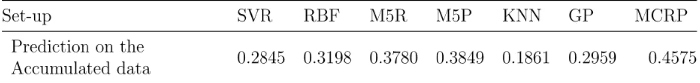
For the first point of interest, we consider how the algorithms performed in cities from Europe against cities from the USA. We use the Mann-Whitney U-test to determine whether the predictive error for both daily and accumulated data is affected by the continent. Table

9 shows the pvalues for the Mann-Whitney U-test at the 5% significance level for all

algo-rithms. We can clearly see that there is no significant difference between cities from Europe

and the USA, withpvalues ranging from 0.1861 to 0.4575. Therefore, we are confident that

the predictive error of each algorithm is similar between Europe and the USA. 19

(21)

(a) Delft - GP (b) Delft - RBF (c) Delft - MCRP

(d) Gorlitz - GP (e) Gorlitz - RBF (f) Gorlitz - MCRP

(g) Des Moines - GP (h) Des Moines - RBF (i) Des Moines - MCRP

(j) Portland - GP (k) Portland - RBF (l) Portland - MCRP

Figure 2: Comparison of GP’s, RBF’s and MCRP’s predictive performance on four cities using the daily rainfall. The dashed line represents the actual daily rainfall amount (0.1mm) and the solid line represents the predicted daily rainfall amount (0.1mm).

(22)

(a) Delft - GP (b) Delft - RBF (c) Delft - MCRP

(d) Gorlitz - GP (e) Gorlitz - RBF (f) Gorlitz - MCRP

(g) Des Moines - GP (h) Des Moines - RBF (i) Des Moines - MCRP

(j) Portland - GP (k) Portland - RBF (l) Portland - MCRP

Figure 3: Comparison of GP’s, RBF’s and MCRP’s predictive error (RMSE) on four cities after accumulating the daily rainfall. The dashed line represents the actual rainfall amount (0.1mm) after the accumulation of rainfall and the solid line represents the predicted rainfall amount (0.1mm).

(23)

S. Cramer et al. / Expert Systems With Applications 00 (2017) 1–27 22 Table 9: Mann-Whitney U-test results (pvalue) to determine whether each algorithm performed statistically

better in one continent.

Set-up SVR RBF M5R M5P KNN GP MCRP

Prediction on the

Accumulated data 0.2845 0.3198 0.3780 0.3849 0.1861 0.2959 0.4575

Table 10: The linear correlation coefficient (r) andpvalue for European cities, in order to determine whether

there is sufficient evidence that a relationship exists between a data set property and an algorithm’s predictive error, measured by CV(RMSE). Thepvalue is shown in brackets below the correlation coefficient. Significant

relationships (p <0.05) are shown in bold.

Data set property SVR RBF M5R M5P KNN GP MCRP

% of dry days 0.05 0.08 0.10 0.08 0.33 0.08 0.30

(0.8197) (0.7421) (0.6823) (0.7262) (0.1493) (0.7454) (0.2049)

Average dry spell 0.21 0.23 0.24 0.23 0.40 0.23 0.39

(0.3763) (0.3350) (0.3106) (0.3261) (0.0822) (0.3315) (0.0907)

Average wet spell 0.15 0.13 0.10 0.12 -0.17 0.13 -0.10

(0.5187) (0.5900) (0.6617) (0.6110) (0.4606) (0.5811) (0.6744) Annual rainfall 0.07 0.10 0.11 0.12 0.30 0.10 0.22 (0.776) (0.6898) (0.6402) (0.6137) (0.1965) (0.6805) (0.3434) Volatility 0.24 0.26 0.27 0.25 0.50 0.26 0.47 (0.3091) (0.2652) (0.2572) (0.2904) (0.0256) (0.2745) (0.0349) Highest intensity 0.40 0.44 0.45 0.42 0.72 0.42 0.65 (0.0776) (0.0536) (0.0442) (0.0670) (0.0003) (0.0641) (0.0019) Interquartile range -0.57 -0.59 -0.61 -0.58 -0.74 -0.58 -0.70 (0.0089) (0.0057) (0.0042) (0.0069) (0.0002) (0.0071) (0.0006)

We compare the percentage of wet/dry days, the average spell length, average daily rainfall, volatility, highest intensity and interquartile range for each city against the predic-tive error for each algorithm, establishing whether a strong correlation exists. The results for both Europe and the USA are presented in Tables 10 and 11, showing the Pearson product-moment linear correlation coefficient for each pair of algorithm and data set

prop-erty. Additionally, we include thep value, in order to determine whether there is a

statisti-cally significant relationship between the predictive error and the descriptive statistics. The values highlighted in bold indicate a statistically significant relationship at the 5% level.

Looking at both Table 10 and 11, we can see a mixed picture of relationships and it appears that there are some strong correlations between climatic aspects and predictive error. In order to assist the comparison against our points of interest, we discuss separately the relationships for European and the USA cities, because we have already determined the significant differences in climate between these two sets of cities in Section 2.

When considering if the percentage of dry days is significantly correlated with predictive error, we observe that across Europe, little relationship exists with the correlation coefficient

r values ranging between 0.05 to 0.33 looking at Table 10. Therefore, there is some positive

relationship, but not enough for a statistically significant result. On the other hand looking 22

(24)

S. Cramer et al. / Expert Systems With Applications 00 (2017) 1–27 23 Table 11: The linear correlation coefficient (r) andpvalue for the USA cities, in order to determine whether

there is sufficient evidence that a relationship exists between a data set property and an algorithm’s predictive error, measured by CV(RMSE). Thepvalue is shown in brackets below the correlation coefficient. Significant

relationships (p <0.05) are shown in bold.

Data set property SVR RBF M5R M5P KNN GP MCRP

% of dry days -0.3 -0.31 -0.35 -0.31 -0.26 -0.30 -0.48

(0.1818) (0.1663) (0.1124) (0.1628) (0.2461) (0.1683) (0.0230)

Average dry spell -0.40 -0.41 -0.46 -0.41 -0.39 -0.42 -0.47

(0.0644) (0.0550) (0.0304) (0.0557) (0.0692) (0.0539) (0.0276)

Average wet spell -0.06 -0.07 -0.06 -0.07 -0.16 -0.08 0.22 (0.8009) (0.7645) (0.7759) (0.7616) (0.4729) (0.7362) (0.3151) Annual rainfall -0.42 -0.40 -0.33 -0.33 -0.27 -0.37 0.14 (0.0496) (0.0656) (0.1323) (0.1310) (0.2216) (0.0926) (0.5288) Volatility -0.36 -0.37 -0.42 -0.36 -0.35 -0.37 -0.32 (0.0955) (0.0861) (0.0546) (0.0964) (0.1107) (0.0894) (0.1486) Highest intensity 0.46 0.48 0.51 0.48 0.43 0.49 0.08 (0.0298) (0.0247) (0.0151) (0.0247) (0.0463) (0.0199) (0.7085) Interquartile range -0.40 -0.41 -0.43 -0.42 -0.45 -0.44 -0.03 (0.0676) (0.0606) (0.0450) (0.0489) (0.0361) (0.0396) (0.9100)

at Table 11, we observe r values between -0.26 to -0.48 within the USA, indicating that

for MCRP there is some correlation at the 5% significance level. Interestingly, with all algorithms having a negative correlation, the drier the climate the smaller the CV(RMSE). This difference in the findings for Europe and the USA makes sense, given that the USA has longer dry spell lengths compared to Europe, which is far more changeable. Therefore, from a predictive perspective it is easier to predict constant behaviour over a period of time rather than more sporadic behaviour.

When we consider the volatility we observe a completely different picture. Across

Eu-rope, there is a positive correlation with r values ranging between 0.24 and 0.50. In the

case of KNN and MCRP there is sufficient evidence to suggest a relationship exists at the 5% significance level, indicating the CV(RMSE) increases with higher levels of volatility. However, we observe the opposite relationship looking at the correlation values from the

USA, with r values between -0.32 and -0.42. Unlike Europe, we do not see any algorithm

exhibiting a significant relationship, but we see a slight improvement in CV(RMSE) the higher the volatility. One reason for this negative relationship is because the volatility is closely linked with the balance of dry and wet days, which links back to the spell lengths previously discussed. This underlying relationship means that the higher the volatility, the drier the climate is, and we have shown that drier climates are negatively correlated to the CV(RMSE) for cities in the USA.

Finally, when we consider the rainfall intensities, we notice a broadly similar pattern

across Europe and the USA. Across Europe, we observer values in the range of 0.40 to 0.72

with MCRP, KNN and M5R having a significant correlation. Similarly, within the USA

we observe r values in the range of 0.08 to 0.51, with all algorithms having a significant

correlation except for MCRP. These findings are expected for both geographic areas since 23

(25)

we noticed when analysing the data earlier that achieving the highest peaks is very difficult. The relationships noticed with the intensity and volatility are reflected by the interquartile range, which is heavily dependent on both aspects. We witness a reduction in CV(RMSE) from data exhibiting a larger interquartile range, which makes sense for rainfall data series as the cities with larger interquartile ranges have a more consistent climate. We witness this alongside the improvement in rainfall prediction coverage as previously shown in Table 6.

From examining the different climates based on our four points of interest, we notice that the patterns of results for all algorithms in general are different when we compare results for Europe and the USA. There are two benefits we can see from the analysis. The first one is the benefit the accumulation of rainfall has across both geographic areas, with no significant difference in the predictive error of all algorithms between Europe and the USA. Secondly, the binary problem of dry and wet days appears to have been satisfactorily solved, since the predictive error is not significantly affected in general regardless of the balance between dry and wet days. However, we do witness that some relationships are present between climatic indicators and predictive error for some algorithms, namely, volatility, maximum potential rainfall intensities and the interquartile range. Future research should look into capturing these shocks of the model, which fall outside of the interquartile range, including the known range of the training set. Capturing this behaviour should result in the algorithms performing equally in predictive power across all climates.

The experimental results show that the use of machine learning-based intelligent sys-tems has greatly assisted in the prediction of rainfall for rainfall derivatives. Moreover, by producing better rainfall predictions, the pricing accuracy should increase. This has two implications to the field of rainfall derivatives. Firstly investors can become more confident within the market. Secondly as result of the first point, more users can be attracted to trade in the market, increasing the liquidity of the rainfall derivatives market.

7. Conclusion

This paper extensively evaluates a recently proposed method for predicting accumulated rainfall amounts using a sliding window (Cramer et al., 2015), within the problem of rain-fall derivatives, dealing with complex data sets which exhibit extreme rainrain-fall values and volatility. The method was proposed in order to predict the accumulated rainfall amounts (rather than predicting daily rainfall) for such applications as financial securities (e.g. rain-fall derivatives), where prices of contracts are based on accumulated amounts over a given period. By accumulating rainfall allows for patterns that were previously unrecognised and helps deal with the problem of discontinuity and extreme rainfall values.

We applied a range of well established machine learning algorithms and the most com-monly used techniques within rainfall derivatives, to predict rainfall before and after ac-cumulating the rainfall amounts. The motivation for this paper is to make the process of rainfall prediction simpler and more effective, overcoming some of the difficulties that ex-ist within the daily rainfall time series. Hence, this paper has two main contributions: (i) extensively testing the accumulation of rainfall on several machine learning techniques, and

(26)

(ii) evaluating whether the combination of the data accumulation and algorithms is affected across varying climates.

We evaluated the predictive error on 42 cities from around Europe and the USA before and after accumulating daily rainfall using a sliding window. Our results show that there is sufficient evidence that accumulating rainfall amounts leads to superior predictive power than predicting using the daily amounts. Furthermore, when applied to the accumulated data, Radial Basis Functions, Support Vector Regression and Genetic Programming were the best algorithms in general, where Radial Basis Functions statistically outperformed the most commonly used approach of Markov chain extended with rainfall prediction. As each algorithm used the same parameter set for all data sets, we can not guarantee that the optimal parameter set was used. This was to show that a robust parameter set is effective, but there were occasions where the regression models were mis-specified during training.

We did notice that there exists some relationship between climatic features and predictive error in general across all algorithms, namely the volatility of rainfall, maximum rainfall intensities and the interquartile range of rainfall. Most importantly, we do not witness any significant difference in the algorithms’ predictive error across Europe and the USA. Additionally, the problem of discontinuity within the rainfall time series is satisfactorily solved by accumulating rainfall amounts.

Within the broad area of intelligent systems, we have shown that machine learning algorithms can be applied to difficult problems such as rainfall prediction. The application of seven machine learning algorithms reported in this work shows that intelligent systems are useful complementing the results reported by Liao et al. (2012); Patel et al. (2015); Cosma et al. (2017), who all show the benefit that machine learning-based intelligent systems can have on real-life scenarios.

Future work will include testing on variable lengths of training and testing data sets to assist in predicting the accumulated rainfall for a single contract, rather than a “one-size-fits-all” approach. Moreover, modifying the tuning procedure to produce a parameter setting customised to a data set’s climate. We could also test the concept on other data sets that exhibit a pattern of similar time series to rainfall. Finally, another research direction is to extend the algorithms to overcome the weaknesses identified earlier in Section 6.2.

References

Akaike, H. (1974). A new look at the statistical model identification. IEEE Transactions on Automatic Control,19, 716–723.

Broomhead, D. S., & Lowe, D. (1988). Multivariable Functional Interpolation and Adaptive Networks. Complex Systems 2, (pp. 321–355).

Buishand, T. A. (1978). Some remarks on the use of daily rainfall models. Journal of Hydrology, 36, 295–308.

Cabrera, B. L., Odening, M., & Ritter, M. (2013). Pricing rainfall futures at the CME. Journal of Banking & Finance,37, 4286 – 4298.

Cao, M., Li, A., & Wei, J. Z. (2004b). Precipitation modeling and contract valuation. The Journal of Alternative Investments, 7, 93–99.

Chang, C.-C., & Lin, C.-J. (2011). LIBSVM: A library for support vector machines. ACM Transactions on Intelligent Systems and Technology, 2, 27:1–27:27.