Civil Engineering Journal
Vol. 5, No. 8, August, 2019Development of Traffic Volume Forecasting Using Multiple
Regression Analysis and Artificial Neural Network
Ramadan Duraku
a, Riad Ramadani
b*a University of Prishtina, Faculty of Mechanical Engineering, Department of Traffic and Transport, 10 000 Prishtina, Kosovo. b University of Prishtina, Faculty of Mechanical Engineering, Department of Design and Mechanisation , 10 000, Prishtina, Kosovo.
Received 09 March 2019; Accepted 09 July 2019
Abstract
The purpose of this study is to develop a model for traffic volume forecasting of the road network in Anamorava Region. The description of the current traffic volumes is enabled using PTV Visum software, which is used as an input data gained through manual and automatic counting of vehicles and interviewing traffic participants. In order to develop the forecasting model, there has been the necessity to establish a data set relying on time series which enables interface between demographic, socio-economic variables and traffic volumes. At the beginning models have been developed by MLR and ANN methods using original data on variables. In order to eliminate high correlation between variables appeared by individual models, PCA method, which transforms variables to principal components (PCs), has been employed. These PCs are used as input in order to develop combined models PCA-MLR and PCA-RBF in which the minimization of errors in traffic volumes forecasting is significantly confirmed. The obtained results are compared to performance indicators such R2, MAE, MSE and MAPE and the outcome of this undertaking is that the model PCA-RBF provides minor errors in
forecasting.
Keywords: Traffic Volume; Forecasting Model; Multiple Regression Analysis; Artificial Neural Network; Principal Component Analysis.
1.
Introduction
Transport planning requires the use of demographic and social economic variables in order to estimate traffic volume forecasting for a particular country or region [1]. In recent years traffic volume has been increasing by an annual average of 4.13% in the main road network of Anamorava region, causing a decrease in the service level and resulting in longer travel times, in a decrease of road safety etc. [2]. Road traffic plays an important role in this region because it is the one connection to the country and through its community trips are carried out. This increase has a direct impact in traffic volume forecasting which can be done through forecasting methods such as: econometric regressions, travel-demand modelling and neural network modelling [3].
Many researchers have dealt with the development of models to traffic volume forecast. Morf and Houska (1958) [4] have developed a model to forecast the traffic in rural areas in the State of Illinois (USA) using Multiple Regression Analysis (MLR) method.Tennant (1975) has developed a model for the assessment of traffic volumes in rural area in developing countries including some socio-economic variables, using land and principles of traffic generation in the region of Mali in Kenia. MLR method is used in order to find variables with higher impact which has been the employment followed by vehicle ownership [5].
* Corresponding author: [email protected]
http://dx.doi.org/10.28991/cej-2019-03091364
© 2019 by the authors. Licensee C.E.J, Tehran, Iran. This article is an open access article distributed under the terms and conditions of the Creative Commons Attribution (CC-BY) license (http://creativecommons.org/licenses/by/4.0/).
Then, Neveu (1982)has developed a number of models involving elasticity parameters in MLR in order to forecast traffic volumes as Annual Average Daily Traffic (AADT) for different roads category. Variables included in the model are: population, number of households, vehicle ownership and employment [6]. This model has been improved by Fricker and Saha (1987) increasing the number of variables in order to forecast traffic volume in the rural roads of Indiana State (USA). The traffic volume has been considered as a dependent variable, whilst 13 variables have been taken as independent at the level of country and region [7].
Varagouli et al. (2005) have developed a model to forecast by MLR method taking into consideration some independent variables which affect the travel demand of the prefecture of Xanthi in Northern Greece [8].
Pupavac (2014) has developed two models to forecast traffic volume on Croatian motorways using econometric methods involving five independent variables and two other dependent variables [9]. Semeida (2014) has developed models according to MLR and Generalized Linear Modelling (GLM) in order to forecast traffic demand for countries with low number of populations, the case of Port Said Governorate in Egypt. He has concluded that GLM model provides the best results in forecasting the number of trips [10].
Nevertheless, methods based on MLR have their defects because dependencies between variables are given in linear form. Thus, with the intention to overcome non-linearity in last decades, neural network has been used in the field of traffic and transport engineering applying various algorithms [11]. ANN has the strong ability to approximate the function and through them the non-linearity between variables and historic traffic data can be reduced compared to other methods [12].
Adamo (1994) has developed a model to estimate AADT using Artificial Neural Network (ANN) and MLR, concluding that the ANN has slightly outperformed the MLR approach [13]. Sharma et al. (2000) have developed models for traffic volume forecast according to traditional methods and ANN in interstates roads with high-volume in Minnesota. The given research is extended to the low-volume roads. By comparing them, it has been found out that ANN provides better results [14].
Tang et al. (2003) have used adapted time-series, neural network, nonparametric regression, and Gaussian maximum methods in order to develop models for traffic volume forecasting by day of the week, by month and AADT for the entire year 1999. The research has been completed using traffic data for the period 1994-1998 in Hong Kong [15]. Duddu and Pulugurtha (2013) have developed a model using statistical methods and ANN taking into account demographic principles in order to estimate link-level AADT based on characteristics of the land use, in the city of Charlotte, North Carolina [16].
Islam et al. (2018) has applied ANN methods and support vector machines (SVM) to estimate AADT based on variables: road geometry, existing counts and local socio-economic data, applying various algorithms for supervised learning of ANN [17]. Park et al. has applied Radial Basis Function (RBF) neural network for traffic volumes forecasting in a freeway. The obtained results show that RBF gives suitable function and it requires less time for calculations [18]. Zhang et al. (2007) have used a combination based on Principal Component Analysis (PCA) and Combined Neural Network (CNN) for short-term traffic flow forecasting. With the transformation of variables using PCA method, Principal Components (PCs) have been used as input data for CNN enabling dimensional reduction of input variables and the size of CNN network. The results according to this approach have been much better than the typical Error Back-Propagation neural network (BPNN) with the same data [19]
.
Doustmohammadi and Anderson (2016) develop the models that can accurately estimate AADTs within a small or medium sized community. Variables that uses these models are a combination of roadway and socio-economic factors within a quarter-mile buffer of the desired count location. These models were tasted and validated to accurately predict across different communities of similar size to support AADT estimation on desired roadways in different communities [20].
Raja et al. (2018) develop a model using linear regression using known AADTs and collection of socio-economic and location variables as a means to estimate the AADT. This model relied on five independent variables nearby population, number of households in the area, employment in the area, population to job ratio and access to major roads. This model is use to estimate traffic volume on low-volume rural and local roads for 12 counties in Alabama [21].
Khan et al. (2018) develops AADT estimation models for different roadway functional classes with two machine learning techniques: Artificial Neural Network (ANN) and Support Vector Regression (SVR). The models aim to predict AADT from short-term counts. The comparison reveals the superiority of SVR for AADT estimation for different roadway functional classes over all other methods [22].
Fu et al. (2016) develops an alternative and low-cost approach for estimating annual average daily traffic values (AADTs) and the associated transport emissions for all road segments in a country. This is achieved by parsing and processing commonly available information from existing geographical data, census data, traffic data and vehicle fleet
data. It was found that AADT estimation based on a neural network performs better than traditional regression models [23].
In this study the model for traffic volume forecasting in Anamorava region is developed. Initially, the current status of traffic volumes in this region has been determined using PTV Visum software, which uses data on traffic volumes as an input. The model is developed according to MLR and ANN methods including 12 independent original variables. In order to develop a model with better performance, respectively to have less errors in forecasting, PCA, in which original variables are transformed in non-correlated PCs, is employed. Those PCs are afterwards used as an input for development of model according to combined PCA-MLR and PCA-ANN methods. In each one of the four methods some significant models have been found, but, based on statistical analysis only the best ones have been selected. Furthermore, comparing those models according to performance indicators, it has been found out that the best model for traffic volume forecasting has resulted to be the one according to PCA-RBF method. The current model is accomplished according to parameters in given region and it can be used in practice.
2.
Materials and Methods
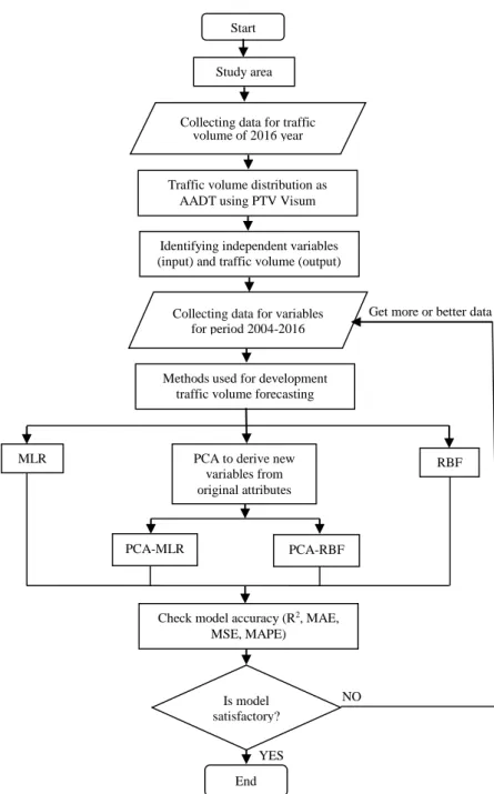
This section provides methodology and processing stages for the development of the model for forecasting traffic volume by flow chart as presented by Figure 1.
Figure 1.The flow chart of the developed models
Start
Collecting data for traffic volume of 2016 year
Traffic volume distribution as AADT using PTV Visum
Identifying independent variables (input) and traffic volume (output)
Collecting data for variables for period 2004-2016
Methods used for development traffic volume forecasting
MLR PCA to derive new RBF
variables from original attributes
PCA-MLR PCA-RBF
Check model accuracy (R2, MAE,
MSE, MAPE) Is model satisfactory? End NO YES Study area
2.1.Study Area
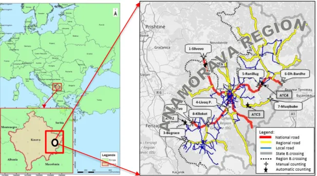
The development of the model for traffic volume forecasting has been carried out in Anamorava region, which is situated in the Peninsula Balkan and South East of Kosovo, Figure 2. The given region includes six municipalities (Gjilan, Vitia, Kamenica, Partesh, Kllokot, and Ranillug) with an area of 1331 km2 [24]. The road network of this region
consists of national, regional and local roads. The two national road represent major transportation links between the capital city of this region Gjilan with the other regions of Kosovo and neighbor’s municipality of Kosovo. Also, in Figure 2 shows the map of traffic flow measurement stations (automatic and manual) for this study.
Figure 2. Anamorava region and its current road network
2.2.Data Collection
In order to develop a model for traffic volumes forecasting, an overview of traffic load distribution on the road network is required. In this regard, data were collected for one work day (15.05) as well as weekend day (21.05) during the period of time 07.00 a.m until 19.00 p.m in May of 2016 with an intention not to require application of a weekly nonlinear coefficient of trips. Traffic counting is accomplished manually (MTC) in eight locations as well as automatic counting (ATC) which took place at four locations (1-Slivovo, 2-Sojevo, 3-Ranillug and 4-Pasjan), with former being suitable for the application of forecasting methods as presented in this paper, Figure 1. There are 11523 interviews conducted based on face-to-face method which consists of 19.43% of the total flow of 59317 vehicles. After the research, counting and interviewing was done using the MS Exel program. Using the ratio between counting and interviewing, it is possible to find traffic volume for 12 h. Converting traffic from 12h into 24h has been done by employing related correction coefficient gained Ke,Kint and Kcon which shows traffic volumes as AADT [25]. The final origin-destination (O-D) matrix is established by processing and interconnecting counting and interviews of traffic participants for the period of time 24h, by Equation 1.
(24 ) 12 int
(
/ 24 )
matrix h e con
OD
VOL
K
K
K
vehicle
h
(1) Where ODmatrix(24h)– is the origin-destination matrix of trips realized by vehicle in time interval 24 hour, VOL12– is the number of vehicles counting in 12 hours interval, Ke– is the passenger car space equivalent,K
int=VOL12/I12is the coefficient of interview calculated by number of vehicles counting (VOL12) and number of interview (I12) realized in 12 hours interval and Kcon=VOL24/VOL12– is the converting coefficient of traffic volume from 12 hours to 24 hours.Once the description of traffic volumes has been made through modelling at PTV Visum, then it was done comparing the results with data count for each location separately. In the beginning there was a discrepancy, but with the application of the balancing process which is based on the production and assign by equilibrium method using the TFlowFuzzy algorithm it was achieved that these discrepancies would achieve satisfactory values [26]. Calibration was carried out with GEH test application [27]. Referring to the results achieved, it is seen that the 8 locations where they were taken for analysis, 7 or 86% of them fulfil the condition defined by GEH <5, as presented in Table 1.
Table 1. Summary of GEH test indicators
Evaluation aggregate
GEH: Avg. 2
GEH:<5.0 86%
Deviation:Avg. 3%
Deviation: Avg. weighed 4%
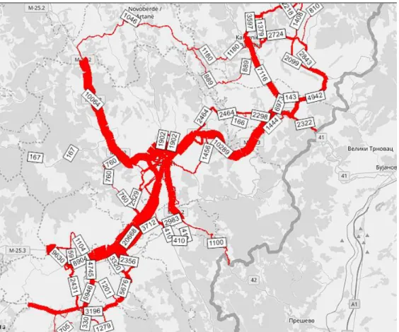
Once this matrix is imported to PTV Visum software, the development of the macro model is enabled through which the generation and the distribution of traffic volumes conducted for unit of vehicle category on current road network of this region is obtained, Figure 3 [28]. The model includes 373 nodes, 948 connections and 13 zones.
Figure 3. Traffic volume distribution on current main road network
In order to develop a model for traffic volumes forecasting, initially, 12 demographic and socio-economic variables which have an impact in traffic demand have been identified. Afterwards, the data-set is established for these variables in time historic format for the period 2004-2016 [29], through which it was enabled to establish dependence with traffic volumes. The data-set related to the traffic volumes is established for four locations in which automatic counting are static.
2.3.Modelling Methods
In order to develop the model for traffic volume forecasting MLR and ANN methods as well as combined methods PCA-MLR and PCA-ANN are employed [30].
2.3.1. Multiple Regression Analysis
Multiple regression analysis is a statistical method used to investigate the relation between variables based on mathematical model that called regression model. MLR explains dependent variable yi as the result of changing in k, independent variables (x1, x2,...,xik) to certain size and direction, where i represents number of years, k is the number of independent variables. A schematic form of MLR method is shown in Figure 4.
Figure 4. Scheme of MLR method
The general form of MLR is expressed by Equation 2 [33]:
0 1 1 1 2
...
i i i k ik i
y
x
x
x
(2)Where, yi: is dependent variable, β0: isintercept, β1,β2,...,βk: are regression coefficients, xik: are independent variables and εi: is error associated during regression.
Here it is important to verify whether two or more independent variables are strongly correlated, known as the multicollinearity phenomenon. If this happens then it has taken measures for its elimination, because it affects negatively to the predictive ability of the model. Different techniques are used to eliminate it. As a technique that is commonly used is that "stepwise" because during model selection includes statistical indicators VIF and DW [31]. This technique works on the principle of adding and removing variables in each iteration.
In case we have only two alternative models with a level of significance p<0.05, choosing one of them as best is done by evaluating parameters according to the standard error by applying the "Sum of Squares" method to the prediction. Testing is done through various statistical indicators R, R2, Adjusted R, ANOVA through test F, t-test,
residual analysis etc. The final selection of one of the significant models is done by selecting the minimum value that ANOVA gives under the Fisher F-test. But in cases where a significant number of models is greater than two but finite, for selecting the best model, are using selection criteria as well: Akaike Information Criterion (AIC), Amemia Prediction Criterion (APC), Mallow`s Prediction Criterion (Cp), Schwarz Bayesian Criterion (SBC) [32].
2.3.2. PCA-MLR method
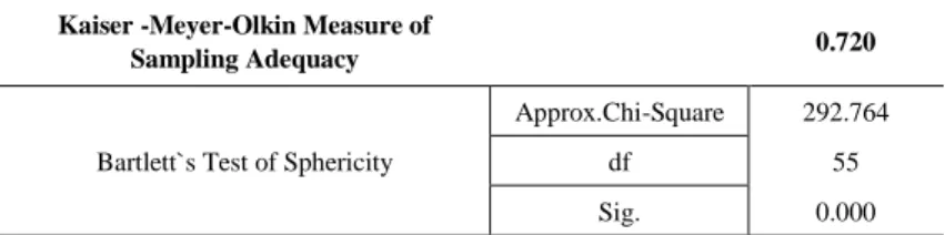
The PCA method is part of the multivariate statistical nonparametric method, through which the elimination of the high correlation between the initial variables (multicollinearity phenomenon) and improved the predictive ability of the model, namely reducing error in prediction. This method is used to summarize the information collected by several observed variables that are strongly correlated with each other and by reducing them to a smaller number of factors or by forming a new data set that contains a number of principal components (PCs). These obtained PCs are non-correlated and they get linear weight like a combination of original variables and they are also used as input for MLR method. Moreover, PCA method relies on three basic steps: estimation of suitability of data, extracting main components and rotation of vectors. In order to justify PCA method it is necessary to verify suitability data through tests according to Kaiser-Meyer-Olkin (KMO>0.5) and Bartlett Test (p<0.05) [33]. The next step is to extract PCs, which are obtained by calculating the eigen values of the matrix. They PCs which have eigen values greater than 1 (eigen>1) should be taken into consideration during the construction of the model where the order is made going from the largest variance to the smallest. The last step is the rotation of factors through which new factors can be acquired and interpreted.
The analysis through PCA-MLR enables a combination of PCA and MLR methods in order to establish mutual relation between dependent variable yiandPCs which are obtained as the result of multiplying original independent variables xik by eigenvectors. A schematic form of PCA-MLR is shown in Figure 5.
Figure 5. Scheme of PCA-MLR method
The general analytical form of PCA-MLR is presented in Equation 3 [33]:
0 1 1 2 2 0 1 ( ... ) n i k k j j i k y
PC
PC
PC
PC u
(3)Where, β0: isintercept, β1, β2,...,βk: are the regression coefficients, PC1, PC2,...PCn: are basic components, ui: is the error associated during regression.
2.3.3. Artificial Neural Network
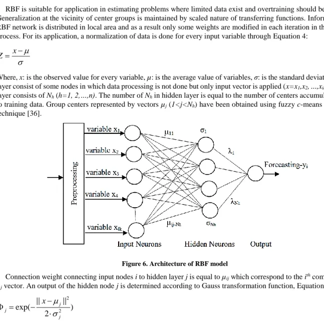
ANN shows high level interface adaptation of non-linear processing neuron elements for parallel processing of data through simple way. ANN method avoids detailed mathematical analysis and it is used to overcome non-linearity which is present through input and output variables used to develop the model [34]. This method is also used to learn, to adjust, to generalize, to investigate and to reproduce linear and nonlinear relation between variables etc. [35]. There are several variants of ANN method. Based on processing information they are classified into: feed forward (Single Layer Perceptron, Multilayer Perceptron, Radial Basis Network) and back forward (Competitive Networks, Kohonen`s SON, Hopfield Network, ART models). One variant is RBF neural network which works in feed-forward error-back propagation network, and it is widely used. RBF has a simple topology and it consists of three layers: input layer, hidden layer and output layer, Figure 6. Nodes contained in hidden layer have non-linear transfer function with radial base, while nodes in output layer have linear transfer function.
RBF is suitable for application in estimating problems where limited data exist and overtraining should be avoided. Generalization at the vicinity of center groups is maintained by scaled nature of transferring functions. Information on RBF network is distributed in local area and as a result only some weights are modified in each iteration in the training process. For its application, a normalization of data is done for every input variable through Equation 4:
x
Z
(4)Where, x: is the observed value for every variable, µ: is the average value of variables, σ: is the standard deviation. Input layer consist of some nodes in which data processing is not done but only input vector is applied (x=x1,x2, ...,xik). Hidden layer consists of Nh (h=1, 2,…,n). The number of Nh in hidden layer is equal to the number of centers accumulated used to training data. Group centers represented by vectors µj (1<j<Nh) have been obtained using fuzzy c-means algorithm technique [36].
Figure 6. Architecture of RBF model
Connection weight connecting input nodes i to hidden layer j is equal to µij which correspond to the ith component of µj vector. An output of the hidden node j is determined according to Gauss transformation function, Equation 5:
2 2
exp(
)
2
j j jx
(5)Where, x: is the input vector for neuron, µj : is the centric value of basis node j in hidden layer , ||x- µj ||: is the Euclidean distance between a center vector and the set of data points, σj2: is the variance of the function for each of the centers (j)
or range of influence of the Gaussian function from centers µj and is calculated according to Equation 6 [36]:
2 1
1
,
3
h N j j i i hN
1
j
N
h (6)In Equation 6, factor σjis equal to 1/3 of the value of the number of nodes Nhand average distance from group centers. Connection of nodes from hidden layer j in output node layer is defined by its weight λj. The value y in the output of network is shown by Equation 7:
1 h N j j j
y
(7)The weights λj are calculated after getting minimal error of network between the value at output y and the desired value yd based on the data-set of network training. Furthermore, in order to train network and find out weights λj, the problem should be solved through unconstrained optimization method Equation 8:
1 ( ) N i i d i MinimizeE
y y
(8)Where: N: is the total number of cases of training sample, λj are weights which connection of nodes from hidden layer j in output node layer, yi -value in output layer, yi
d– desired value in output layer. In order to solve the problem of minimization of error descent gradient algorithm is used as shown in [37].
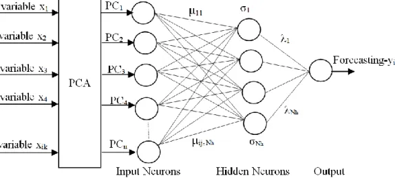
2.3.4. PCA-RBF Method
The combination of PCA and RBF methods, PCA-RBF method is combined through which there is possibility to get the relation between the dependent variable yi and obtained uncorrelated PCs as input variables in RBF [38]. For this reason, we initially apply the PCA method as a preprocessor to the neural network according to the RBF method to eliminate high correlation between original variables xik. It is known fact that PCA operates with the data that function in the linear form, while that of the ANN for data that have a nonlinear form. The idea here is when they are used together, to have the opportunity to effectively cover the linear and nonlinear part of the forecast. Moreover, the combination according to this approach will minimize the complexity of problem of training in network. The way of functioning is presented in Figure 7.
Figure 7. Architecture of PCA-RBF model
3.
Results and Discussions
In order to develop a model to forecast the traffic volume there is the necessity to fulfil some preconditions such as variance, normality tests,graphical method and description of variables. The analysis starts with variance of testing of data-set for dependent variable yi for locations such Slivove, Sojeva, Ranillug and Pasjan. In order to estimate the variance on traffic volumes for above mentioned locations Levene test is used through which homogeneity is verified for the level of significance (Sig.=0.429>Sig.=0.05), as presented in Table 2.
Table 2. Variance test of homogeneity for dependent variable yi.
Levene Statistic Sig.
0.867 0.429
This test with the value 0.867 it means that the variance of homogeneity between locations has approximate value. For the given locations, testing of normality of data is done through Shapiro-Wilk test, in which the value of the coefficients ß next to each location has turned to be at significant level Sig>0.05, as presented in Table 3.
Table 3. Normality test for dependent variable yi
Type of road Location Number of observed Kolmogorov Test Shapiro Wilk Test ß Sig. Normality
National All locations together 39 0.112 0.200 0.05 fulfilled
National Slivovo 13 0.823 0.013 0.05 fulfilled
National Sojevo 13 0.888 0.093 0.05 fulfilled
National Ranillug 13 0.914 0.207 0.05 fulfilled
Regional Pasjan 13 0.826 0.014 0.05 fulfilled
This result proves that there is no necessity to do transformation of data according to any function (log, sqrt etc.). Therefore, in order to simplify the problem, based on results of two tests which was fulfilled in general only Slivove location, which represents other locations, is treated.
Apart from this, graph method is also used to verify the dependency of any independent variable xik to the dependent variable yi in which it results in variable x12 (number of vehicles registered in Anamorava level), which shows a tendency and a dependency which is more sustainable with dependent variable and expectation for increase for the period of time 2004 – 2016.
In this regard, a statistical description is accomplished for the presentation of variables which take place in developing model to traffic volume forecasting, are shown in Table 4.
Table 4. Basic descriptive statistics for variables
Name of variable Symbol N Min Max Mean Std.Dev
Traffic Volume y 1 6325 10439 7449 1240
State Population x1 12 1786282 1891906 1846303 37473
State Household x2 12 278915 338618 311062 17863
State Employment x3 12 236181 340911 290450 33631
State Vehicle Registration x4 12 179157 336942 249102 52192
Consumer Price Index x5 12 77 101 90 9
Gross Domestic Product x6 12 3006100 5984900 4431790 1072114
Per Capita Income x7 12 1763 3356 2507 562
Gasoline Price x8 12 0.840 1.160 1.015 0.027
Region Population x9 12 240502 254723 248583 5045
Region Household x10 12 48999 51442 50504 685
Region Employment x11 12 32270 43692 37302 3983
Regional Vehicle Registration x12 12 29031 53806 39419 8514
The development and the estimation of significant model is done by employing the above-mentioned methods and the SPSS software. In the following, the results of the model according to each method are presented and discussed.
3.1. Results by MLR
The outcome of the matrix of correlation shows that each k of independent variable (x=x1,…,x12) in relation to dependent variable y fulfils condition that the values of correlation coefficient are (r>0.8). Apart from this, it is obvious that independent variables have high correlation (dependency) and as a result there is multi-co linearity phenomenon. This phenomenon has been overcome by using stepwise technique in SPSS software which is functioning according to forward and backward method in order to add and remove variables, resulting in 14 significant candidate models at the p<0.05 level and two non-significant models with p>0.05. Summarized results are given in Table 5.
Table 5. Model summary
Model Predictor variables R R2 Adjusted R2 Std. Error Sig.F Change Durbin Watson
1 x1 0.723a 0.523 0.480 894.36176 0.005 0.557 2 x2 0.738a 0.545 0.503 873.93719 0.004 0.805 3 x3 0.866a 0.751 0.728 646.79968 0.000 1.197 4 x4 0.925a 0.856 0.843 491.76565 0.000 1.113 5 x5 0.803a 0.645 0.613 771.38572 0.001 0.568 6 x6 0.890a 0.792 0.773 590.74995 0.000 0.658 7 x7 0.901a 0.813 0.796 560.79044 0.000 0.725 8 x8 0.461a 0.212 0.141 1149.63385 0.113 0.363 9 x9 0.723a 0.523 0.480 894.34210 0.005 0.557 10 x10 0.663a 0.440 0.389 969.14285 0.013 0.617 11 x11 0.888a 0.789 0.770 594.69288 0.000 1.063 12 x12 0.933a 0.871 0.859 465.53011 0.000 1.338 13 x4, x8 0.947a 0.897 0.877 435.47191 0.000 1.822 14 X6, x8 0.938a 0.880 0.856 470.61794 0.000 1.385 15 X7, x8 0.940a 0.883 0.860 464.40321 0.000 1.364 16 X8, x11 0.919a 0.844 0.812 537.03697 0.000 1.627 a.Predictors: x1,x2,x3,x4,x5,x6,x7,x8,x9,x10,x11,x12,(x4,x8), (x6,x8), (x7,x8), (x8,x11). b.Dependent variable: y
Based on the results of the table above it is seen that model 12 gives the maximum value of the determination coefficient (R2) of 0.871 (what it means 87.1% of the variance of the variance of the response variable (ds) explained
by the model). Adjusted R2=0.859 shows that 85.9% of variation of dependent variable is explained by the variation of
independent variables. In this regard, the sustainability of the model according to Durbin-Watson (DW=1.338) test has also been verified, which is not within the interval of auto correlation of 1.5 to 2.5.
However, as we have already explained above, only through this coefficient we are not sure whether we have found the best model because we have some significant models. Therefore, we apply the selection criteria where the results are presented in Table 6.
Table 6. Summary of selection criteria
Model df1 df2 Akaike Information
Criterion Amemia Prediction Criterion Mallows' Prediction Criterion Schwarz Bayesian Criterion 1 1 11 178.527 0.650 2.000 179.657 2 1 11 177.927 0.621 2.000 179.056 3 1 11 170.101 0.340 2.000 171.231 4 1 11 162.976 0.197 2.000 164.106 5 1 11 174.681 0.484 2.000 175.811 6 1 11 167.745 0.284 2.000 168.874 7 1 11 166.391 0.256 2.000 167.521 8 1 11 185.055 1.074 2.000 186.185 9 1 11 178.527 0.650 2.000 179.656 10 1 11 180.615 0.763 2.000 181.745 11 1 11 167.917 0.287 2.000 169.047 12 1 11 161.551 0.176 2.000 162.681 13 2 10 160.576 0.164 3.000 162.271 14 2 10 162.594 0.192 3.000 164.289 15 2 10 162.249 0.187 3.000 163.944 16 2 10 166.027 0.250 3.000 167.722
Based on these results the model 12 is selected as the best because it gives smaller value by selection criteria, compared with other candidate models. To compare the goodness of fit of model 12 and intercept only-model (i.e., mean value of the response variable) is used the ANOVA test as shown in Table 7.
Table 7. ANOVA test
Model SumSquares Df. Mean Square F Sig.(p<0.05)
Regression 16071147.64 1 16071147.64 74.157 0.000b
Residual 2383901.12 11 216718.28
Total 18455048.76 12
In this regard, it has also been proven the significance of model according to ANOVA, F-test (F=74.157) with reliability value 95% respectively the p-value is less than 0.01 (p=0.000<0.05), which shows that the alternative hypothesis is verified Ha: where at least one of the independent variables is statically significant and different from zero while rejecting the hypothesis H0: at 99% confidence level.
Table 8. Coefficient table
B Std. Error t Sig.(p<0.05) Tolerance VIF
Constant 2091.432 635.437 3.291 0.000
x12 0.136 0.016 8.611 0.001 1.000 1.00
Also, by results in Table 8 for t-test (t=8.611) it is clear that variable x12is a significant variable with the value of reliability 95% that p-value is less than 0.05 and it may be used to develop a model in order to forecast the traffic volumes. Apart from this, the value of the coefficient (VIF=1<10) shows that multi-co linearity does not exist. Therefore, MLR model expressed through variables x12 is presented by Equation 9:
12
2091.432 0.136
Y
x
(9)Equation 9 shows that the variable x12 has a positive impact in traffic volumes, which means that by increasing the level of motorization in the level of Anamorava region the value of dependent variable “traffic volume” is also increasing. The weakness of this model is that as a consequence of high correlation, as a result number of independent variables drastically falls in model development.
3.2. Results by PCA-MLR
In order to include more variables in developing the model combination of methods PCA and MLR is used. In order to apply this method, some necessary conditions are fulfilled according to Kaiser-Meyer-Olkin test (KMO=0.720>0.5)
and Bartlett’s test of Sphericity Sig.(p<0.05), as presented in Table 9.
Table 9. KMO and Bartlett`s Test
Kaiser -Meyer-Olkin Measure of
Sampling Adequacy 0.720
Bartlett`s Test of Sphericity
Approx.Chi-Square 292.764
df 55
Sig. 0.000
In order to find the eigenvalues associated to each factor, are necessary to use the phases: before extraction, after extraction and rotation. Before the phase of extraction there are 12 linear components identified within the data set. By using PCA method all original variables are grouped in two factors which are named PC1 and PC2 by eigenvalue bigger than 5% with the variability about 96%, while another PCs which have the value approaching to zero has been removed from the model, because it shows high correlation between each other and means there is presence of multicollinearity.
Based on matrix components, are proved that exists simple correlation or have higher values (higher than 0.9) between all original variables and new PCs. Thus, variables
x
11, x
4, x
7, x
6, x
12, x
3andx
5have high impact in PC1, while variablesx
1, x
9, x
8, x
10andx
2 have more high impact in PC2. While multiplying scores of coefficients (eigenvalues) and values of original variables obtained scores for each PCs as presented by Equations 10 and 11.1 2 3 4 5 6 7 8 9 10 11 12 PC1=0.030 +0.044 x +0.156 x +0.172 x +0.066 x +0.125 x +0.136 x -0.113 x +0.030 x -0.05 x +0.147 x +0.200 x x (10) 1 2 3 4 5 6 7 8 9 10 11 12 PC2=0.177 x +0.150 x -0.037 x -0.064 x +0.120 x +0.023 x +0.02 x +0,379 x +0.177 x +0.224 x -0,019 x -0.118 x (11)
These PCs are used as independent variables in MLR analysis to determine all significant PCs, which could be used in the model. Using stepwise procedure in SPSS software the results are obtained according to this hybrid method as shown in Table 10.
Table 10. Model summary
Model R R2 Adjusted R2 Std Error D.Watson
1 0.948a 0.899 0.879 431.58135 1.486
The results show that the dependent variable has high correlation of obtained PCs and it is qualified as independent variables and R2=0.899 show that 89.9% of dependent variable is explained by non-correlated PCs. Adjusted R2=0.879
show that 87.9% of variation of dependent variable is explained by variation of PCs. Also, it has also been verified the sustainability of the model according to Durbin-Watson (DW=1.486) test which is not within the interval of auto correlation 1.5 to 2.5.
Table 11. ANOVA test
Model SumSquares Df. Mean Square F Sig.(p<0.05)
Regression 16592424.14 2 8296212.07 44.540 0.000b
Residual 1862624.62 10 186262.46
Total 18455048.76 12
It has also been verified by results in Table 11 that the significance of the model according to ANOVA, associated with F-test (F=44.540) the value of reliability 95% respectively the p-value is less than 0.01 (p=0.000<0.05), which indicates that the alternative hypothesis is verified Ha: where at least one of the independent variables is statically significant and different from zero while rejecting the H0: hypothesis at 99% confidence level.
Table 12. Coefficient test
B Std Error t Sig.(p<0.05) Tolerance VIF
Constant 7449.308 119.699 62.234 0.000
PC1 1516.286 205.210 7.389 0.000 0.369 2.713
PC2 -473.241 205.210 -2.306 0.044 0.369 2.713
In this regard, in Table 12 are presented results by t-test (t=7.389 and t=-2.306) that shows the condition of significance is fulfilled for two PCs with values of reliability 95% Sig.(p=0.000<0.05) and Sig.(p=0.044<0.05) used for development of model for traffic volumes forecasting. Apart from this, the value of coefficient (VIF=2.713<10) shows that multi co-linearity does not exist. Thus, the model is expressed through PC1 and PC2 components by Equation 12:
7449.308 1516.286 1 473.241 2
y PC PC (12)
By Equation 12, shows that PC1 component has a positive impact whilst PC2 component has a negative impact in traffic volumes. The advantage of this method is that reduces multicollinearity phenomenon and the complexity of model development, while the disadvantages of this method are that in interpretation between original variables and PCs also the model is developed only in a linear form.
3.3. Results by RBF
In order to develop a model with optimal network, some models of neural network of RBF type according to "trial and errors" technique are designed which differ in numbers of neurons in hidden layer, the way of functioning is activated as well as rules of learning. Before beginning with the training of data-set, normalization of input variables is done. Data in data-set gained in 13 observations (13 years) has been completed in randomly and for training purposes 10 observations are taken or 76.9 %, while for testing 3 observations or 23.1%.
Training data in data set is used to develop a model and to find out weights, while the data of testing are used to find errors and to prevent overtraining in the training process. The determination of the number of neurons of RBF network is done according to automatic way. The number of neurons at input layer is 12, while the number of neurons at hidden layer is 5, whilst the number of neurons at output layer is 1.
Neurons at output layer mean forecasted traffic volumes. Activation function “softmax” is applied to connect number of neurons from hidden layer to the output layer. For output layer, “identity” is used as activation function. In order to
calculate an error, “sum of squares error” is applied. In Table 13, are given the overall results of the model associated with the description of the error generated by the neural network together with the ratio (percentage) of inaccurate predictions during the training and testing phases.
Table 13. Model Summary
Training Sum of Squares Error 0.049
Relative Error 0.011 Training Time 0:00:00.02
Testing Sum of Squares Error 0.038
Relative Error 0.104 Dependent variable y.
Table 13 shows that the error in training is (SSE=0.049) which shows the significance of model for forecasting. Error when doing testing is (SSE=0.038) which means that the model is not overtraining. Furthermore, percentage in inaccuracy in forecasting training is 0.011 (or 1.1%) while in testing is 0.104 (or 10.4%). The dependency of values observed with those forecasted is provided in Equation 13:
15.96 1.01
y x (13)
From Equation 13, R2=0.986 is gained and it shows that observations of forecasted values have high dependence and
that this is suitable model for forecasting.
3.4. Results by PCA-RBF
In order to minimize error in forecasting combined method PCA and RBF is used. Similarly, like the PCA-MLR method, required tests for PCA are given in Table 9. In this case obtained PCs are used as an input in neural network of RBF type. In order to prove the validity of PC the sample of data-set is divided in two parts: training and testing one. Before starting with training of data-set, normalization of PC is done using Equation 4. Data in the data-set cover 13 observations (13 years) chosen in random bases, for training 9 observations are taken which is 69.2%, while for testing purposes 4 observations are taken which is 30.8%. Selection of optimal network architecture is done in automatic way selecting 2 neurons in input layer, 5 neurons in hidden layer and 1 neuron in output layer. The neuron in output layer means also variable on traffic volume yi.
Activation function “softmax” is applied at neurons in hidden layer, while "identity" is used at neurons in output layer. In order to calculate an error, “sum of squares error” is applied. The summary of obtained results related to the inaccuracies of the forecasts are shown in Table 14.
Table 14. Model Summary
Training Sum of Squares Error 0.005
Relative Error 0.001 Training Time 0:00:00.02
Testing Sum of Squares Error 0.010
Relative Error 0.026 Dependent variable y.
Results shown in Table 14 show that an error in training is (SSE=0.005), while an error in testing is (SSE=0.010)
which means that the model is stronger and it is not over trained. Furthermore, the percentage in inaccuracy in forecasting training is 0.001 (or 0.1 %) while at testing is 0.026 (or 2.6%). Dependency of values observed with the ones forecasted is reflected in Equation 14:
49.21 1.01
y x (14)
From Equation 14, R2=0.997 is gained and it shows the measured observations with the values of forecasting with
high dependency and the model is suitable for forecasting.
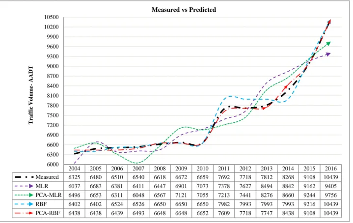
The results gained according to four methods mentioned above in graph way are shown in Figure 8. In Figure 8, a black curve shows the data measured for the traffic volume by automatic counting, also, volumes of traffic forecasted by (MLR-orange, PCA-MLR-green, RBF-blue, PCA-RBF-red) methods are shown. Comparing the results in the graph shows that the volumes measured with the ones forecasted on traffic are approximate by all four methods, but more sustainable results are given by PCA-RBF method; the red curve in red complies with the black one.
Figure 8. Comparison of values measured with traffic volume forecasting
4.
Performance Comparisons of Models
In order to determine which one of the four methods used provides higher accuracy in developing a model on traffic volume forecasting, models are established and compared with each other based on performance indicators such is: R2,
MAE, RMSE and MAPE [33]. In order to calculate those indicators, forecasted data are included Fi as well as the ones measured Ai. The obtained results are shown in Table 15.
Table 15. Performance comparisons of MLR, RBF, PCA-MLR and PCA-RBF
Performance Indicators MLR PCA-MLR RBF PCA-RBF
Adjusted R2 0.99839 0.99980 0.99874 0.99996
MAE 361 106 336 50
RMSE 428 150 370 70
MAPE 4.25 1.38 4.46 0.70
The results of indicators show that models relied on neural network compared to the ones based on linear regression provide lower error in forecasting because models of neural network are expressed in the form of non-linearity. This was expected due to the relation between independent variables and traffic volumes in the form on non-linearity. The best model is offered by PCA-RBF method because an error in forecasting is lower. Therefore, the model developed according to this method is suggested to be used for traffic volumes forecasting for Anamorava region.
5.
Conclusion
This study the development of the model for traffic volume forecasting in Anamorava region is presented. Current state of distribution of traffic volumes is expressed by employing PTV Visum software which serves as starting point to develop forecasting model. With the intention to develop a model, 12 variables with an impact in generating traffic volumes are identified, establishing a data-set in the form of time series. Applying these variables and employing methods relied in regression and neural network, certain significant models are developed.
Based on the analysis of the results of these models, it has been found out that the model based on neural PCA-RBF is the best one because it provides lower value error in traffic volume forecasting. Therefore, this model can be used also in the preparation of the transport planning strategy for this region.
2004 2005 2006 2007 2008 2009 2010 2011 2012 2013 2014 2015 2016 Measured 6325 6480 6510 6540 6618 6672 6659 7692 7718 7812 8268 9108 10439 MLR 6037 6683 6381 6411 6447 6901 7073 7378 7627 8494 8842 9162 9405 PCA-MLR 6496 6653 6311 6048 6567 7121 7055 7213 7441 8276 8660 9244 9756 RBF 6402 6402 6524 6526 6650 6650 6650 7982 7993 7993 7993 9216 10439 PCA-RBF 6438 6438 6439 6493 6648 6648 6652 7609 7718 7747 8438 9108 10439 6000 6300 6600 6900 7200 7500 7800 8100 8400 8700 9000 9300 9600 9900 10200 10500 T ra ff ic V o lu m e -AADT Measured vs Predicted
6.
Acknowledgment
The authors expressed thanks to the students at the Department of Traffic and Transport Engineering/University of Prishtina for their assist in conducting counting and interviews in main road network of Anamorava region.
7.
Conflict of Interests
The authors declare no conflict interest.
8.
References
[1] Ortuzar, J.D., and Williamson, L.G. “Modelling Transport, Fourth Edition”. United Kingdom: John Wiley and Sons Ltd (2011). [2] Ministry of Infrastructure-Directorate of Roads. “Data for Traffic Volumes by Automatic Counting for the Period 2004-2016”.
Prishtina.
[3] Fu, Miao, J. Andrew Kelly, and J. Peter Clinch. “Estimating Annual Average Daily Traffic and Transport Emissions for a National Road Network: A Bottom-up Methodology for Both Nationally-Aggregated and Spatially-Disaggregated Results.” Journal of Transport Geography 58 (January 2017): 186–195. doi:10.1016/j.jtrangeo.2016.12.002.
[4] Morf, F.T., and Houska, V.F. “Traffic Growth Pattern on Rural Areas”. Highway Research Board Bulletin 194. (1958). [5] Tennant, B. “Forecasting Rural Road Travel in Developing Countries from Land Use Studies”. Transport Planning in Developing
Countries, Proc., Summer Annual Meeting, Planning and Transport Research and Computation Company, Ltd., Univ. of Warwick, Coventry, Warwickshire, England.Accession Number: 00148235, 153-163. (1975).
[6] Neveu, A.J. “Quick Response Procedure to Forecast Rural Traffic”. Transportation Research Record 944, (1982). 47-53. [7] Fricker, Jon, and Sunil Saha. “Traffic Volume Forecasting Methods for Rural State Highways” (1986).
doi:10.5703/1288284314120.
[8] Varagouli, E.G., Simos, T.E., and Xeidakis, G.S. “Fitting a Multiple Regression Line to Travel Demand Forecasting: The Case
of Prefecture of Xanthi, Northern Greece”. Mathematical and Computer Modelling, Vol. 42, (2005). 817-836. doi: 10.1016/j.mcm.2005.09.010.
[9] Miksic, Stefica, Maja Miskulin, Brankica Juranic, Zeljko Rakosec, Aleksandar Vcev, Dunja Degmecic, et al. “Depression And Suicidality During Pregnancy.” Psychiatria Danubina 30, no. 1 (March 15, 2018): 85–90. doi:10.24869/psyd.2018.85. [10] Semeida, A.M. “Derivation of Travel Demand Forecasting Models for Low Population Areas: The Case of Port Said
Governorate, North East Egypt”. Journal of Traffic and Transportation Engineering, Vol. 1, No. 3. (2014). 196-208. doi:10.1016/S2095-7564(15)30103-3.
[11] Karlaftis, M.G., and Vlahogianni, E.I. “Statistical Methods versus Neural Networks in Transportation, Research: Differences, Similarities and Some Insights”. Transportation Research an International Journal Part Emerging Technologies. Vol. 19, No. 3 (2011), 387–399. doi:10.1016/j.trc.2010.10.004.
[12] Yun, S.-Y., S. Namkoong, J.-H. Rho, S.-W. Shin, and J.-U. Choi. “A Performance Evaluation of Neural Network Models in Traffic Volume Forecasting.” Mathematical and Computer Modelling 27, no. 9–11 (May 1998): 293–310. doi:10.1016/s0895-7177(98)00065-x.
[13] Adamo, M. “Estimation of Annual Average Daily Traffic Volumes Using Neural Networks”. Faculty of Science, Laurentian University (1994).
[14] Sharma, S.C., Lingras, P., Liu, G.X., and Xu, F. “Estimation of Annual Average Daily Traffic on Low-Volume Roads Factor Approach Versus Neural Networks”. Transportation Research Record, Journal of the Transportation Research Board, Vol. 1719, (2000). 103–111. doi:10.3141/1719-13.
[15] Tang, Y.F., Lam, W.H.K., and Pan, L.P. “Comparison of Four Modelling Techniques for Short-Term AADT Forecasting in Hong Kong”. Journal of Transport Engineering, Vol. 129, No. 3. (2003); 271–277. doi:10.1061/(ASCE)0733-947X (2003)129:3(271).
[16] Duddu, V.R., ASCE, A.M., Pulugurtha, S.S., and ASCE, M. “Principle of Demographic Gravitation to Estimate Annual Average Daily Traffic: Comparisons of Statistical and Neural Network Models”. American Society of Civil Engineers. Vol. 139, No. 6, (2013). 585-595. doi:10.1061/(asce)te.1943-5436.0000537.
[17] Sababa, I. “Estimation of Annual Average Daily Traffic and Missing Hourly Volume Using Artificial Intelligence”. A Thesis Presented to the Graduate School of Clemson University. (2016).
[18] Park, B., Messer, C.J., and Urbanik, T. “Short-term Freeway Traffic Volume Forecasting Using Radial Basis Function Neural Network”. Transportation Research Record, Journal of the Transportation Research Board, Vol. 1651, No. 1, (1998). 39-47. doi:10.3141/1651-06.
[19] Zhang, X.I., and He G.G. “Forecasting Approach for Short Term Traffic Flow Based on Principal Component Analysis and Combined Neural Network”. Systems Engineering -Theory & Practice, Vol. 27, No. 8, (2007), 167–171. doi: 10.1016/S1874-8651(08)60052-6.
[20] Doustmohammadi, M., and M. Anderson. "Developing direct demand AADT forecasting models for small and medium sized urban communities." Int. J. Traff. Transp. Eng 5, no. 2 (2016): 27-31.
[21] Raja, P., Doustmohammadi,M., and Anderson, M. D. “Estimation of Average Daily Traffic on Low Volume Roads in Alabama”. International Journal of Traffic and Transportation Engineering (2018), 7(1): 1-6.
[22] Khan, Sakib Mahmud, Sababa Islam, MD Zadid Khan, Kakan Dey, Mashrur Chowdhury, Nathan Huynh, and Mohammad Torkjazi. “Development of Statewide Annual Average Daily Traffic Estimation Model from Short-Term Counts: A Comparative Study for South Carolina.” Transportation Research Record: Journal of the Transportation Research Board 2672, no. 43 (November 8, 2018): 55–64. doi:10.1177/0361198118798979.
[23] Fu, M., Kelly, J. A, and Clinch J. P. “Estimating annual average daily traffic and transport emissions for a national road network: A bottom-up methodology for both nationally-aggregated and spatially-disaggregated results”. Journal of Transport Geography 58 (2017) 186–195. doi.org/10.1016/j.jtrangeo.2016.12.002.
[24] Kosovo Census Atlas. “Geographic and Administrative Division of Kosovo”. Kosovo Statistics Agency. (2013), Prishtina. [25] Alonso, B., Mouram, J. L., Ibeas, A., and Romero J. P. “Estimation of Annual Average Daily Traffic with Optimal Adjustment
Factors”. Proceedings of the Institution of Civil Engineers Transport, Vol. 168, No. TR5, (2015), 406–414. doi:10.1680/tran.12.00074 Paper 1200074.
[26] PTV AG. (2008). “How to work with TFlow Fuzzy”. Official Manual, PTV Vision Visum, Karlsruhe.
[27] TII Publications PE-PAG-02015. (2016). “Project Appraisal Guidelines for National Roads Unit 5.1 – Construction of Transport Models”. Transport Infrastructure Ireland (TII).
[28] PTV Visum15 User’s manual. PTV Group. (2016), Karlsruhe, Germany. [29] Kosovo Agency Statistic. General Statistics of Kosovo (2016), Pristine.
[30] Feng, X., Gan, T., Wang, X., Sun, Q., and Ma, F. “Feedback Analysis of Urban Densities and Travel Mode Split”. International Journal of Simulation Modelling, Vol. 14, No. 2, (2015), 349-358. doi:10.2507/IJSIMM14(2)C09.
[31] Rawlings,J.H., Pantula, S.G., Dickey, D.A. “Applied Regression Analysis: A Research Tool”. Second Edition. Springer. (1998). [32] Pelosi, M.K., and Sandifer, TH.M. Elementary Statistics from Discovery to Decision. John Willey&Sons. ISBN-13:
978-0471401421.
[33] Kosun, C., Tayfur, G., and Celik, H.M. “Soft Computing and Regression Modelling Approaches for Link-Capacity Function”. International Journal of Non-Standard Computing and Artificial Intelligence, Vol. 2, (2016), 129–140, doi:10.14311/NNW.2016.26.007.
[34] Pamuła, T. “Neural Networks in Transportation Research – Recent Applications”. Transport Problems, Vol. 11, No. 2, (2016), 27-36. doi:10.20858/tp.2016.11.2.3.
[35] Yu., B., Wang Y.T., Yao J.B., and Wang J.Y. “A Comparison of the Performance of ANN and SVM for the Prediction of Traffic Accident Duration”. International Journal of Non-Standard Computing and Artificial Intelligence”. Neural Network World 3/2016, 271–287. doi:10.14311/NNW.2016.26.015.
[36] Karim A., Adeli H., and ASCE, F. “Radial Basis Function Neural Network for Work zone Capacity and Queue Estimation”. Journal of Transportation Engineering, ASCE, Vol. 129, No. 5, 494-503. doi:10.1061/(ASCE)0733-947X (2003)129:5(494). [37] Saric, T., Simunovic, G., and Simunovic, K. “Use of Neural Networks and Simulation of Steel Surface Roughness”. International
Journal of Simulation Modelling, Vol. 12, No. 4, (2013), 225-236. doi:10.2507/IJSIMM12(4)2.241.
[38] Wey, C.C. “RBF Neural Networks Combined with Principal Component Analysis Applied to Quantitative Precipitation Forecast for Reservoir Watershed During Typhoon Periods”. Journal of Hydrometeorology, Vol. 13, (2012), 722-734. doi:10.1175/JHM-D-11-03.1.
![Figure 5. Scheme of PCA-MLR method The general analytical form of PCA-MLR is presented in Equation 3 [33]:](https://thumb-us.123doks.com/thumbv2/123dok_us/1293250.2673359/6.892.95.763.103.1220/figure-scheme-pca-method-general-analytical-presented-equation.webp)