Nonparametric inference with directional and linear data

(1)

PhD Dissertation

Nonparametric inference with

directional and linear data

Eduardo García Portugués

Departamento de Estatística e Investigación Operativa Universidade de Santiago de Compostela

(2)

(3)

Nonparametric inference with

directional and linear data

Eduardo García Portugués

(4)

de Ciencia e Innovación, Project 10MDS207015PR fromDirección Xeral de I+D da Xunta de Galicia and IAP network StUDyS from Belgian Science Policy. The author gratefully acknowl-edges the computational resources used at the SVG cluster of the CESGA Supercomputing Center that allowed to run most of the simulations.

(5)

Informe de los directores

Don Wenceslao González Manteiga, Catedrático del Departamento de Estatística e Investigación Operativa de la Universidade de Santiago de Compostela y Doña Rosa M. Crujeiras Casais, Profesora Contratada Doctora en el mismo departamento, como directores de la tesis titulada “Nonparametric inference with directional and linear data”

Por la presente,_declaran

Que la tesis doctoral presentada por Don Eduardo García Portugués es idónea para ser presen-tada, de acuerdo con el artículo 41 del Reglamento de Estudios de Doctorado, por la modalidad de compendio deartículos, en los que el doctorando tuvo participación en el peso de la inves-tigación y su contribución fue decisiva para llevar a cabo este trabajo.

Y que está en conocimiento de los coautores, tanto doctores como no doctores, participantes en los artículos, que ninguno de los trabajos reunidos en esta tesis serán presentados por ninguno de ellos en otra tesis de doctorado, lo que firmamos bajo nuestra responsabilidad.

En Santiago de Compostela, a 3 de septiembre de 2014.

Los directores:

Prof. Dr. Wenceslao González Manteiga Prof. Dr. Rosa M. Crujeiras Casais El doctorando:

Eduardo García Portugués

(6)

(7)

Agradecimientos

Quiero comenzar estos agradecimientos expresando mi profunda gratitud por el apoyo recibido por parte de mis directores, Wenceslao González Manteiga y Rosa M. Crujeiras, durante todo el proceso de realización de esta tesis doctoral. A Wences le agradezco el haber despertado mi interés por la estadística en mis últimos años de licenciatura, la confianza que depositó en mí desde mis primeros pasos como investigador y la continua motivación que me ha transmitido. Estoy muy agradecido a Rosa por su apoyo diario, tanto profesional como personal, a lo largo de estos años. Valoro especialmente sus innumerables y exhaustivas revisiones críticas, que han servido para perfeccionar notablemente el trabajo desarrollado en esta tesis. La verdad es que me siento enormemente afortunado por haberla tenido como codirectora. I would like also to thank Ingrid Van Keilegom for her hospitality and her guidance in research during my stay at Louvain-la-Neuve.

Gracias a mi madre y a mi padre, a vosotros os lo debo todo en esta vida. Gracias también a mi familia por haberme apoyado en esta y en otras etapas y, en especial, a mi abuela Isabel Del Río Galza y a mi abuelo Rafael Portugués Carrera. Que esta tesis sirva como mi pequeño homenaje a los grandes esfuerzos que ambos realizaron por el bienestar de la familia.

Finalmente, agradezco a mis compañeros del Departamento de Estadística e Investigación Ope-rativa y de la Facultad de Matemáticas por los buenos momentos pasados durante estos años.

Santiago de Compostela, 3 de septiembre de 2014. Eduardo García Portugués

(8)

(9)

List of Figures

1.1 Polar coordinates in Ω₁ and spherical coordinates in Ω₂ (just an octant of the sphere is represented for a better display). . . 2 1.2 Von Mises densities on Ω1 and Ω2. From right to left, densities corresponding to q= 1

withκ1andκ2and toq= 2 withκ1andκ2, respectively. The parameters areµ= (0q,1),

κ1= 2 andκ2= 5, with0q denoting a vector ofqzeros. Samples of sizen= 250 are drawn. 4

1.3 From right to left, densities corresponding to: MS 3π

2 ,5,0, 1 2,− 3 4, 3 2 ; density (1.1) with a vM 5₄π,3₂link and marginalsN(0,1) and circular uniform; density (1.1) with a vM(π,7) link and marginals JP 0,1₂,1

and uniform circular; WNT 0,π₆,3₂,1₄,0

. Samples of size

n= 300 are drawn. . . 5 1.4 Diagram with the contributions of the thesis (marked in bold) and a short state of the

art with the main references in the scope of the thesis. Future research lines described in Chapter 8 are included in italics. . . 6 1.5 Rose diagrams for wind direction in station B2 for January 2004 (left), January 2011

(center) and in station A mourela in June 2012 (right). The first two ones show the average SO2 concentration in µg/m3 associated with winds coming from each partition

of the windrose. . . 9 1.6 Number of observed stars per square degree, in galactic coordinates (cell size 2◦×2◦),

extracted from Figure 3.2.1 of Perryman (1997). The higher concentrations of stars are located around the equator (galactic plane) and two spots that represent the Orion’s arm (left) and the Gould’s Belt (right). . . 11 1.7 Number of hectares burnt in 1985–2005 in each watershed delineated by Barros et al.

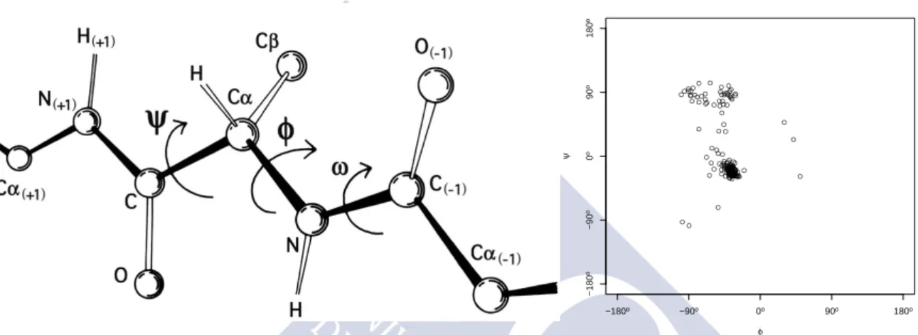
(2012) (left plot) and main orientation of a wildfire obtained from the PC1 of the perime-ter (right plot; extracted from Barros et al. (2012)). . . 12 1.8 Representation of the dihedral angles in the primary protein structure (left, adapted

from Richardson (2011)) and Ramachadran plot of the dihedral angles of the alanine-alanine-alanine segments contained in theProteinsAAA object of Fernández-Durán and Gregorio-Domínguez (2013). . . 13 1.9 View of theSlashdot website on July 27, 2014. . . 14 2.1 Locations of monitoring station (circle) and power plant in Galicia (NW-Spain). Location

of station B2: 7◦ 44’ 10” W, 43◦ 32’ 05” N. Power plant location: 7◦ 51’ 45” W, 43◦ 26’ 26” N. . . 22 2.2 Rose diagrams for wind direction in station B2 for 2004 (left plot) and 2011 (right plot),

with average SO2 concentration. . . 23

2.3 Copula density surfaces. Left plot: J&W copula with von Mises joining density with parameters µ =π and κ = 2. Middle plot: QS-copula with α = (2π)−1. Right plot: reflected Frank copula withα= 10. . . 27

(14)

2.4 Illustration for data reflection for copula density estimation. The central square in each plot corresponds with the original data ranks. Left plot: mirror reflection from Gijbels and Mielniczuk (1990). Right plot: circular-mirror reflection for estimator (2.11). . . . 29 2.5 Density surfaces for the simulation study. Top left: Example 2.1 withµ=π andκ= 2.

Top right: Example 2.2 withµ0 =π,κ0= 5,µ2=π/2 andκ2= 2. Bottom left: Example

2.3 withα= (2π)−1_, _µ

3=π/2 and κ3 = 0.5. Bottom right: Example 2.4 with α= 10,

µ4=π/2 andκ4= 0.5. . . 31

2.6 Boxplots of the ISE×100 for Example 2.1 (top left), Example 2.2 (top right), Example 2.3 (bottom left) and Example 2.4 (bottom right) for n= 500 and different estimation procedures. . . 34 2.7 Circular-linear density estimator for wind direction and SO2concentrations in monitoring

station B2. Left column: 2004. Right column: 2011. . . 37

3.1 Left: contour plot of a von Mises density vM(µ, κ), withµ= (0,0,1) and κ= 3. Right: contour plot of the mixture of von Mises densities (3.14). . . 46 3.2 From left to right: circular-linear mixture (3.15) and corresponding circular and linear

marginal densities, respectively. Random samples of size n= 200 are drawn. . . 52 3.3 From left to right: exact MISE and AMISE for the linear mixture 2₅N 0,₄1+2₅N(1,1) +

1

5N(2,1) and the circular and spherical mixtures (3.14), for a range of bandwidths

be-tween 0 and 1. The black curves are for the MISE, whereas the red ones are for the AMISE. Solid curves correspond to n = 100 and dotted to n = 1000. Vertical lines represent the bandwidth values minimizing each curve. . . 53 3.4 Upper plot, from left to right: exact MISE versus AMISE for the circular-linear mixture

(3.15) forn= 100 andn= 1000. Lower plot, from left to right: spherical-linear mixture (3.15) for n= 100 and n= 1000. The solid curves are for the MISE, where the dashed ones are for the AMISE. The pairs of bandwidths that minimizes each surface error are denoted by (h, g)MISEand by (h, g)AMISE. . . 54

4.1 The effect of the “extra term” inhROT. Left plot: logarithm of the curves of MISE(hTAY),

MISE(hROT) and MISE(hMISE) for sample size n= 250. The curves are computed by

1000 Monte Carlo samples and hMISE is obtained exactly. The abscissae axis

repre-sents the variation of the parameter θ ∈ π

2, 3π

2

, which indexes the reference density

1

2vM ((0,1),2) + 1

2vM ((cos(θ),sin(θ)),2). Right plot: logarithm of hTAY, hROT, hMISE

and their corresponding MISE for different values ofκ, withn= 250. . . 86 4.2 Simulation scenarios for the circular case. From left to right and up to down, models M1

to M20. For each model, a sample of size 250 is drawn. . . 93 4.3 Simulation scenarios for the spherical case. From left to right and up to down, models

M1 to M20. For each model, a sample of size 250 is drawn. . . 95 4.4 Left: density of the wind direction in the meteorological station of A Mourela. Right:

density of the stars collected in the Hipparcos catalogue, represented in galactic coordi-nates and Aitoff projection. . . 97

(15)

List of Figures xiii

5.1 Descriptive maps of wildfires in Portugal with the 102 watersheds delineated by Barros et al. (2012). The left map shows the number of hectares burnt from fire perimeters associated with each watershed. Each fire perimeter is associated with the watershed that contains its centroid. The center map represents the mean slope of the fires of each watershed, where the slope is measured in degrees (0◦ stands for plain slope and 90◦ for a vertical one). Finally, the right map shows watersheds where fires display preferential alignment according to Barros et al. (2012). . . 109 5.2 Random samples ofn= 500 points for the simulation models in the circular-linear case,

withδ= 0.50 (situation with dependence). From left to right and up to down, M1 to M6. M1, M2 and M3 present a deviation from the independence in terms of the conditional expectation; M4 and M5 account for a deviation in terms of the conditional variance and M6 includes deviations both in conditional expectation and variance. . . 116 5.3 p-values from the independence test for the first principal component PC1 of the fire

perimeter and the burnt area (on a log scale), by watersheds. From left to right, the first and second maps represent the circular-linear p-values (PC1 in_R2_{) and their}

cor-rected versions using the FDR, respectively. The third and fourth maps represent the spherical-linear situation (PC1 inR3), with uncorrected and corrected p-values by FDR,

respectively. . . 121 5.4 Left: density contour plot for fires in watershed number 31, the watershed in the second

plot on the left of Figure 5.3 withp-value = 0.000. The number of fires in the watershed isn= 1543. The contour plot shows that the size of the area burnt is related with the orientation of the fires in the watershed. Right: scatter plot of the fires slope and the burnt area for the whole dataset, with a nonparametric kernel regression curve showing the negative correlation between fire slope and size. . . 122 6.1 Density models for the simulation study in the circular-linear case. From left to right

and up to down, models CL1 to CL12. . . 140 6.2 Density models for the simulation study in the circular-circular case. From left to right

and up to down, models CC1 to CC12.. . . 140 6.3 Empirical size and power of the circular-linear (left, model CL1) and circular-circular

(right, model CC8) goodness-of-fit tests for a 10×10 logarithmic spaced grid. Lower surface represents the empirical rejection rate underH0.00and upper surface underH0.15.

Green colour indicates that the percentage of rejections is in the 95% confidence interval of α= 0.05, blue that is smaller and orange that is larger. Black points represent the empirical size and power obtained with the median of the LCV bandwidths. . . 141 6.4 Left: parametric fit (model from Mardia and Sutton (1978)) to the circular mean

orien-tation and mean log-burnt area of the fires in each of the 102 watersheds of Portugal. Right: parametric fit (model from Fernández-Durán (2007)) for the dihedral angles of the alanine-alanine-alanine segments. . . 142 7.1 QQ-plot comparing the quantiles of the asymptotic distribution given by Theorem 7.3

with the sample quantiles for

nh12 Tj n− √ π 4 nh 500 j=1withn= 10 2_{(left) and}_n_{= 5}_×₁₀5 (right). . . 159 7.2 Parametric regression models for scenarios S1 to S4, for circular and spherical cases. . . 161 7.3 Empirical sizes (first row) and powers (second row) for significance levelα= 0.05 for the

different scenarios, with p= 0 (solid line) and p= 1 (dashed line). From left to right, columns represent dimensionsq= 1,2,3 with sample sizen= 100. . . 162 7.4 Significance trace of the local constant goodness-of-fit test for the constrained linear model.163

(16)

8.1 Directional regression models proposed for the simulation study. From left to right and up to down, models used in scenarios S1 to S12, with the first three rows fo the circular versions and the last three for the spherical ones. . . 179 8.2 Directional densities to be considered in the simulation study. From left to right and up

to down, the first two columns represent the directional densities D1 to D6 in the circular case. The corresponsing spherical versions are in the third and fourth columns. For each density, a sample of sizen= 250 is drawn. . . 180 8.3 From right to left: vM(θ, κ) density, rotational kernel density estimators ˆfhLCV,θ and

ˆ

f_h

LCV,ˆθMLE and usual kernel density estimator ˆfhLCV. Sample size isn= 100,θ= (0q,1)

andκ= 2. . . 184 8.4 From right to left: contourplots for copulaCG, copula CGnand empirical copulaCn, for

a sample size of n = 50 with q= −1 and g(θ) = (2πI0(κ))− 1

eκcos(θ−µ) a circular von Mises density withµ= π₂ andκ= 2. . . 189 A.1 Comparison of the asymptotic and empirical distributions of (nhq

ngn) 1

2(T_n−A_n) for

sample sizes n = 5j ×10k, j = 0,1, k = 2,3,4,5. Black curves represent a kernel estimation from 1000 simulations, green curves represent a normal fit to the unknown density and red curves represent the theoretical asymptotic distribution. . . 230 A.2 Empirical size and power of the goodness-of-fit tests for a 10×10 grid of bandwidths.

First two rows, from left to right and up to down: models CL1, CL5, CL7, CL8, CL9 and CL11. Last two rows: CC1, CC5, CC7, CC8, CC9 and CC11. Lower surface represents the empirical rejection rate under H0.00 and upper surface under H0.15. Green colour

represent that the empirical rejection is in the 95% confidence interval of α= 0.05, blue that is lower and orange that is larger. Black points represent the sized and powers obtained with the median of the LCV bandwidths (for model CC1 under H0 is outside

the grid). . . 236 A.3 Upper row, from left to right: parametric fit (model from Mardia and Sutton (1978))

to the circular mean orientation and mean log-burnt area of the fires in each of the 102 watersheds of Portugal; parametric fit (model from Fernández-Durán (2007)) for the dihedral angles of the alanine-alanine-alanine segments. Lower row: p-values of the goodness-of-fit tests for a 10×10 grid, with the LCV bandwidth for the data. . . 239 B.1 From left to right: directional densities for scenarios S1 to S4 for circular and spherical

cases. . . 264 B.2 From left to right: deviations ∆1and ∆2and conditional standard deviation functionσ2

for circular and spherical cases. . . 264 B.3 Densities of the responseY under the null (solid line) and under the alternative

(dashed line) for scenarios S1 to S4 (columns, from left to right) and dimensions

q = 1,2,3 (rows, from top to bottom). . . 265 B.4 Empirical sizes forα= 0.01 (first row), α= 0.05 (second row) andα= 0.10 (third row)

for the different scenarios, withp= 0 (solid line) andp= 1 (dashed line). From left to right, columns represent dimensionsq= 1,2,3 with sample sizen= 100. . . 266 B.5 Empirical sizes forα= 0.01 (first row), α= 0.05 (second row) andα= 0.10 (third row)

for the different scenarios, withp= 0 (solid line) andp= 1 (dashed line). From left to right, columns represent dimensionsq= 1,2,3 with sample sizen= 250. . . 267 B.6 Empirical sizes forα= 0.01 (first row), α= 0.05 (second row) andα= 0.10 (third row)

for the different scenarios, withp= 0 (solid line) andp= 1 (dashed line). From left to right, columns represent dimensionsq= 1,2,3 with sample sizen= 500. . . 268

(17)

List of Figures xv

B.7 Empirical powers for the different scenarios, withp= 0 (solid line) and p= 1 (dashed line). From top to bottom, rows represent sample sizesn= 100,250,500 and from left to right, columns represent dimensionsq= 1,2,3. . . 269

(18)

(19)

List of Tables

2.1 MISE×100 for estimating the circular-linear density in Examples 2.1 and 2.2. Relative efficiencies for JWSP, JWNP, CSP and CNP are taken with respect to JWP. . . 33 2.2 MISE×100 for estimating the circular-linear density in Examples 2.3 and 2.4. . . 33 4.1 Comparative study for the circular case, with sample size n = 500. Columns of the

selector • represent the MISE(•)×100, with bold type for the minimum of the errors. The standard deviation of the ISE×100 is given between parentheses. . . 94 4.2 Ranking for the selectors for the circular and spherical cases, for sample sizes n =

100,250,500,1000. The higher the score in the ranking, the better the performance of the selector. Bold type indicates the best selector. . . 94 4.3 Comparative study for the spherical case, with sample size n = 500. Columns of the

selector • represent the MISE(•)×100, with bold type for the minimum of the errors. The standard deviation of the ISE×100 is given between parentheses. . . 96 4.4 Ranking for the selectors for dimensionsq= 3,4,5 and sample sizen= 1000. The larger

the score in the ranking, the better the performance of the selector. Bold type indicates the best selector. . . 96 4.5 Directional densities considered in the simulation study. . . 100 4.6 Comparative study for the circular case, with up to down blocks corresponding to sample

sizes 100, 250 and 1000, respectively. Columns of the selector• represent the MISE(•)× 100, with bold type for the minimum of the errors. The standard deviation of the ISE×100 is given between parentheses. . . 101 4.7 Comparative study for the spherical case, with up to down blocks corresponding to sample

sizes 100, 250 and 1000, respectively. Columns of the selector• represent the MISE(•)× 100, with bold type for the minimum of the errors. The standard deviation of the ISE×100 is given between parentheses. . . 102 4.8 Comparative study for higher dimensions with sample sizen= 1000: up to down blocks

correspond to dimensionsq= 3,4,5. Columns of the selector•represent the MISE(•)× 100, with bold type for the minimum of the errors. The standard deviation of the ISE×100 is given between parentheses. . . 103 5.1 Proportion of rejections for theR2n,Un,λ4∗n,TnLCVandTnBLCVtests of independence for

sample sizesn= 50,100,200 for a nominal significance level of 5%. For the six different models the values of the deviation from independence parameter are δ = 0 (indepen-dence), 0.25 and 0.50. Each proportion was calculated usingB= 1000 permutations for each ofM = 1000 random samples of sizensimulated from the specified model. . . 118

(20)

5.2 Proportion of rejections for theR2n,Un,λ4∗n,TnLCV andTnBLCV tests of independence for

sample sizes n = 500,1000 for a nominal significance level of 5%. For the six different models the values of the deviation from independence parameter are δ = 0 (indepen-dence), 0.25 and 0.50. Each proportion was calculated usingB= 1000 permutations for each ofM = 1000 random samples of sizensimulated from the specified model. . . 119 5.3 Computing times (in seconds) for TLCV

n and TnBLCV as a function of sample size and

dimension q, with q = 1 for the circular-linear case and q = 2 for the spherical-linear case. The tests were run withB= 1000 permutations and the times were measured in a 3.5 GHz core.. . . 119 6.1 Empirical size and power of the circular-linear and circular-circular goodness-of-fit tests

for models CL1–CL12 and CC1–CC12 (respectively) with significance levelα= 0.05 and different sample sizes and deviations. . . 141 7.1 Specification of simulation scenarios for model (7.3). . . 161 7.2 Fitted constrained linear model on the Slashdot dataset, with R2 = 0.25. The

signifi-cances of each coefficient are lower than 0.002. . . 164 8.1 Simulation scenarios for comparing the bandwidth selectors. fSN is the Skew Normal

distribution of Azzalini (1985), while the rest of notations can be seen in Subsection 4.5.1.181 A.1 Notation for the densities described in Tables A.2 and A.3. . . 231 A.2 Circular-linear models. . . 233 A.3 Circular-circular models. . . 234 A.4 Empirical size and power of the circular-linear goodness-of-fit test for models CL1–CL12

with different sample sizes, deviations and significance levels. . . 237 A.5 Empirical size and power of the circular-circular goodness-of-fit test for models CC1–

(21)

Chapter 1

Introduction

An introduction to basic concepts and statistical tools for analysing directional data is provided in this chapter. Section 1.1 presents a short introduction to the analysis of directional data and to the most well known directional distributions. The contributions of this thesis are summarized in Section 1.2, with a brief state of the art on nonparametric inference with directional and linear data. Section 1.3 describes the real datasets used along the manuscript. Finally, Section 1.4 presents the thesis distribution and organization, with short abstracts describing the contents of each chapter.

Contents

1.1 What is directional data? . . . . 1

1.2 Contributions of the thesis . . . . 5

1.3 Real datasets . . . . 8 1.3.1 Wind direction . . . 9 1.3.2 Hipparcos dataset . . . 10 1.3.3 Portuguese wildfires . . . 11 1.3.4 Protein angles . . . 12 1.3.5 Text mining . . . 13 1.4 Manuscript distribution . . . . 15 References . . . . 16

1.1 What is directional data?

The term directional data was coined in the first book of Mardia (1972) to refer to data whose support is a circumference, a sphere or, generally, an hypersphere of arbitrary dimension. This kind of data appears naturally in several applied disciplines: proteomics (angles in the structure of proteins; see for example Hamelryck et al. (2012)); environmental sciences (wind direction (Johnson and Wehrly, 1978), direction of waves (Jona-Lasinio et al., 2012)); biology (animal orientation, see Batschelet (1981) for several examples); cyclic phenomena (arrival times at a care unit (Fisher, 1993, page 239), seasonality in freezing and thawing (Oliveira et al., 2013)); astronomy (position of stars, see Sections 1.2.8 and 1.5.3 of Perryman (1997)); image analysis (Dryden, 2005) or even in text mining (analysis of word frequency in texts, see for example Banerjee et al. (2005)). The collection of statistical techniques intended to analyse directional

(22)

data was named as directional statistics by the homonym book of Mardia and Jupp (2000), the revised reprint of Mardia (1972).

Directional observations are represented as points in the Euclidean hypersphere of dimension

q, denoted by Ω_q =

x∈_Rq+1 _:_||_x_||_{= 1} _{(also referred to as}

Sq), where the simplest cases

correspond to the circumference (q= 1) and the sphere (q = 2). Inference with directional data is indeed constrained inference, since all the methods used for statistical analysis should take into account the special nature of Ω_q, something that is not required with the usuallinear (i.e.

Euclidean) data. A pedagogical example that illustrates this problem is the definition of an appropriate directional mean for the simplest situation: for two observationsX1 and X2 in the circumference Ω₁. A first attempt could be to consider the Euclidean mean ¯X = X1+X2₂ , but then ¯X is not guaranteed to belong to Ω₁. Another possibility is to consider polar coordinates (see Figure 1.1), compute the usual mean of the corresponding angles θ1, θ2 ∈[0,2π) and then set the directional mean as the point cos ¯θ,sin ¯θ

, where ¯θ = θ1+θ2

2 . The problem with this approach is that if, for example, θ1 = π₄ and θ2 = 7₄π, then ¯θ =π, which produces an output in the opposite direction of the obvious mean, corresponding this one to ¯θ = 0. A reasonable definition for a directional mean is obtained by X¯

||X¯|| (if ¯X 6= 0, not defined otherwise), see

Mardia and Jupp (2000) for further details.

x2

x1 Ω₁ x= (cosθ,sinθ)

θ

Figure 1.1: Polar coordinates in Ω1 and spherical coordinates in Ω2 (just an octant of the sphere is represented for a better display).

Two main approaches have been followed in the statistical literature for the analysis of direc-tional data, differing in the kind of representation. The first one is based on polar and spherical coordinates (see Figure 1.1) to develop methods which are specifically designed to treat circular and spherical data, respectively, the most common types of directional data in practise. This is the approach followed by the books of Fisher (1993), Jammalamadaka and SenGupta (2001) and Pewsey et al. (2013) for circular data and of Fisher et al. (1993) for spherical. Unfortunately, the extensions of these methods to an arbitrary dimensionq are not straightforward due to the nature of the spherical coordinates for higher dimensions. The second approach relies only in the Cartesian coordinates of the points in Ωq, without assuming any particular dimension and

(23)

1.1. What is directional data? 3

thus ensuring more generality. This is the approach followed in the thesis, except in Chapter 2, where the first one is employed.

Perhaps the most popular directional distribution is thevon Mises-Fisher density (see Watson (1983) and Mardia and Jupp (2000)), or shortly the von Mises. The von Mises density, denoted by vM(µ, κ) (or by vM(µ, κ), ifq = 1 and µ= (cosµ,sinµ)), is given by

fvM(x;µ, κ) =Cq(κ) exp n κxTµo, Cq(κ) = κq−12 (2π)q+12 Iq−1 2 (κ) ,

beingµ∈Ωq the directional mean,κ≥0 the concentration parameter around the mean (κ= 0

gives the uniform density on Ω_q) andI_ν the modified Bessel function of the first kind and order

ν, which can be written as (see equation 10.32.2 of Olver et al. (2010))

Iν(z) = z 2 ν π1/2_Γ_ν₊1 2 Z 1 −1 (1−t2)ν−12eztdt.

This distribution is considered as the Gaussian analogue for directional data for two main reasons. First, it presents the same Maximum Likelihood Estimator (MLE) characterization property that the Gaussian distribution has in the Euclidean case: it is the only directional distribution whose MLE of the location parameter is the directional sample mean (see Bingham and Mardia (1975) for a proof). Second, the von Mises density can be obtained from a random vector normally distributed conditioned to have unit norm. That is, for a normal random vector

X∼ Nq+1 µ, σ2Iq+1 , withµ∈Rq+1\{0} and σ2>0, it happens that Y= X||X||= 1 ∼vM _µ ||µ||, ||µ|| σ2 .

This result shows that the inverse of the concentration parameter κ of a von Mises can be identified with the variance of a multivariate normal with covariance matrix proportional to the identity. See Gatto (2011) for a proof of this result in a more general situation.

Another remarkable directional distribution is the one given by Jones and Pewsey (2005), which is denoted by JP(µ, κ, ψ). Originally motivated for the circular case, its density can be also defined in Ωq for an arbitrary dimension q:

fJP(x;µ, κ, ψ) = |sinh(κψ)|q−12 cosh(κψ) + sinh(κψ)xTµ 1 ψ 2q−12 Γ _q₊₁ 2 P− q−1 2 1 ψ+ q−1 2 (cosh(κψ)) ,

whereµ∈Ω_q is the location parameter,κ≥0 is the concentration around µ,ψ∈_Ris a shape parameter that controls a kind of negative kurtosis with respect to a vM(µ, κ) (ψ <0 stands for more peaked densities whileψ >0 produces flatter ones) andP_νµis the Legendre function of the first kind, order µand degree ν (see equation 14.12.4 of Olver et al. (2010)). This parametric family has the interesting property of containing as particular cases the vM(µ, κ) (corresponding toψ → 0) and, with q = 1 and taking polar coordinates, the Cardioid (ψ = 1), the Wrapped

(24)

Cauchy (ψ = −1) and the Cartwright’s power-of-cosine (ψ < 0, κ → ∞). See Section 2 of Jammalamadaka and SenGupta (2001) for more information on these distributions.

0 0.5 1 0 0.5 1

Figure 1.2: Von Mises densities on Ω1and Ω2. From right to left, densities corresponding toq= 1 with

κ1andκ2and toq= 2 withκ1andκ2, respectively. The parameters areµ= (0q,1),κ1= 2 andκ2= 5,

with0q denoting a vector ofqzeros. Samples of sizen= 250 are drawn.

In many situations, directional random variables appear together with a linear or another direc-tional variable, being the circular-linear (support on the cylinder Ω₁×_R) and circular-circular (support on the torus Ω1 ×Ω1) data the most common situations. See Figure 1.3 for some examples of densities in these supports. For both cases, a semiparametric model for the joint density was proposed in Johnson and Wehrly (1978) and Wehrly and Johnson (1979):

fΘ,X(θ, x) = 2πg(2π(FΘ(θ)±FX(x)))×fΘ(θ)fX(x), (1.1)

being Θ a circular variable with densityfΘ and distribution function FΘ and X either a linear or a circular variable with associated fX and FX. g is a circular density that acts as the link

function between the two marginal densities, given by fΘ and fX, either considering a positive

(negative dependency) or a negative sign (positive dependency) in ±. g can be interpreted in terms of copulas (see Nelsen (2006) for an introduction to copulas), since the copula density of (Θ, X) is given by cΘ,X(u, v) = 2πg(2π(u±v)). Different parametric models can be obtained

from this semiparametric structure, for example the bivariate von Mises model of Shieh and Johnson (2005).

However, not all parametric densities in this context satisfy (1.1). For example, the circular-linear density of Mardia and Sutton (1978) (denoted by MS(µ, κ, m, ρ1, ρ2, σ)) or the circular-circular Wrapped Normal Torus given in Example 7.3 of Johnson and Wehrly (1977) (denoted by WNT(m1, m2, σ1, σ2, ρ)) are parametric densities that do not verify (1.1). The expressions of these densities are, respectively:

fMS(θ, x;µ, κ, m, σ, ρ1, ρ2) =fvM(θ;µ, κ)×fN z;m(θ;µ, κ, m, σ, ρ1, ρ2), σ(1−ρ1−ρ2), fWNT(θ, ψ;m1, m2, σ1, σ2, ρ) = ∞ X p1=−∞ ∞ X p2=−∞ fN(θ+ 2πp1, ψ+ 2πp2;m1, m2, σ1, σ2, ρ), where m(θ;µ, κ, m, σ, ρ1, ρ2) =m+σκ 1

2{ρ₁(cos(θ)−cos(µ)) +ρ₂(sin(θ)−sin(µ))},f_N(·;m, σ) stands for the density of a N(m, σ2) and fN(·,·;m1, m2, σ1, σ2, ρ) represents the density of a bivariate normal with mean vector (m1, m2)T, marginal variances σ21 and σ22 and correlation coefficientρ. Among others, these two distributions will be employed along the different chapters. For example, the last two ones appear in Chapter 6 and the relation (1.1) is crucial for Chapter 2.

(25)

1.2. Contributions of the thesis 5

Figure 1.3: From right to left, densities corresponding to: MS 3₂π,5,0,1₂,−3 4,

3 2

; density (1.1) with a vM 5₄π,3₂ link and marginals N(0,1) and circular uniform; density (1.1) with a vM(π,7) link and marginals JP 0,1₂,1

and uniform circular; WNT 0,π₆,3₂,1₄,0

. Samples of sizen= 300 are drawn.

Finally, it should be noted that directional data also arise related to or as particular cases of more general spaces, as it happens for example in statistical shape analysis (see Dryden and Mardia (1998) and Kendall et al. (1999) for a review on the topic) or when consideringstatistics on Riemannian manifolds(see Bhattacharya and Bhattacharya (2012) and references therein).

1.2 Contributions of the thesis

Parametric methods have played a predominant role in the development of statistical inference for the analysis of directional data (see Mardia (1972) and Watson (1983)). Later publications, such as Fisher (1993), Fisher et al. (1993), Mardia and Jupp (2000), Jammalamadaka and SenGupta (2001) and Pewsey et al. (2013) also devoted much of their attention to the use of parametric techniques. These methods rely on the assumption that a certain parametric hypoth-esis in the stochastic generating process holds. For example, inference on the unknown density of a directional random variable is usually done by assuming a certain density model, up to the determination of some unknown parameters which are estimated from the data. Whereas this procedure leads to optimal results (in terms of efficiency) if the parametric assumption holds, the estimation can be totally misleading if the assumption fails.

On the other hand, nonparametric methods do not rely on strong parametric assumptions on the stochastic generating process, except for some mild smoothness conditions. The main advantage is that nonparametric methods always provide reasonable solutions for inference in general, no matter if a parametric assumption holds or not. Obviously, a nonparametric method is not optimal compared with a parametric competitor designedad hocfor a parametric scenario, but still very useful. For example, the comparison of a parametric and a nonparametric fit leads to a so called goodness-of-fit test, which formally checks if the parametric hypothesis is plausible given the sample information.

The aim of this thesis is to provide new methodological tools for nonparametric inference with directional and linear data. Specifically, nonparametric methods are obtained for both estimation and testing, for the density and the regression curves, in situations where directional random variables are present, that is, directional, directional-linear and directional-directional random variables. In what follows, short states of the art on these topics are given jointly with the contributions of the thesis, referring to the papers providing Chapters 2–7, the main core of the manuscript. See also Figure 1.4 for a diagram with the main references and contributions.

(26)

Nonp

arametric

inference

with

directional

and

linear

d

a

t

a

Density function Directional Directional-linear or directional-directional Regression function Directional predicto r and linear response Linear predictor and directional respo nse Estima tion Hall et al. (198 7) Bai et al. (1988) T a ylo r (2008) Oliveira et al. (2012) Ga rcí a-P o rtugués (2013) F u ture w o rk: Section 8.2 Testing Zhao and W u (2001) Bo ente et al. (2014) F u ture w o rk: Section 8.2 Estima tion Ca rnicero et al. (2013) Ga rcía-P o rtugués et al. (2013a) Ga rcía-P o rtugués et al. (2013b) F ut ure w o rk: Section 8.4 Testing Ga rcía-P o rtugués et al. (2014a) Ga rcía-P o rtugués et al. (2014b) F ut ure w o rk: Section 8.4 Softw are Agostinelli a nd Lund (2013) Oliveira et al. (2014) F uture w o rk: Section 8.3 Estima tio n W ang et al. (2000) Di Ma rzio et al. (2009) Di Ma rzio et al. (2014) Ga rcía-P o rtugués et al. (2014) F uture w o rk: Section 8.1 Testing Deschepp er et al. (2008) Ga rcí a-P o rtugués et al. (2014) Estima tion Bo ente and F raiman (1991) Di Ma rzio et al. (2013) Di Ma rzio et al. (2014) Testing — Figure 1.4: Diagram with the con tributions of the thesis (mark ed in b old) and a short state of the art with the main refer ences in the scop e of the thesis. F uture researc h lines describ ed in Chapter 8 are included in italics.

(27)

1.2. Contributions of the thesis 7

A. Density function. Consider X and Y two directional variables and Z a linear one. Let fX, fX,Z and fX,Y be their directional, directional-linear and directional-directional density functions, respectively.

A.1. Estimation. The objective is the estimation offX,fX,Z andfX,Yby kernel smooth-ing methods. The copula density is also estimated for linear and circular-circular cases.

• State of the art. Kernel density estimation for fX was firstly considered by Hall et al. (1987) and Bai et al. (1988), who established its basic asymptotic properties, and was later studied by Klemelä (2000). Taylor (2008) and Oliveira et al. (2012) proposed bandwidth selection rules for the circular case, the latter based in the asymptotic error expression stated in Di Marzio et al. (2009). For the estimation of the densitiesfX,Z andfX,Y with circular variables, Fernández-Durán (2007) introduced a parametric method based on the copula structure given by Johnson and Wehrly (1978). A fully nonparametric estimation of the copula density employing Bernstein polynomials was given in Carnicero et al. (2013).

• Contributions. A new nonparametric method for estimating circular-linear and circular-circular densities from the estimation of the copula structure of Johnson and Wehrly (1978) is presented in García-Portugués et al. (2013a). The method considers, among other approaches, a modification of the kernel density estima-tor of Gijbels and Mielniczuk (1990). Since this procedure is hardly extensible to higher dimensions, in García-Portugués et al. (2013b) a new kernel density estimator forfX,Z is given, which avoids the estimation via copulas. Exact error

expressions are derived for the density estimators of fX,Z and fX,Y. These ex-pressions are used in García-Portugués (2013) to set up new bandwidth selection rules for the kernel density estimator of fX.

A.2. Testing. The two goals are: i) test if X and Z are independent, i.e., test H0 :

fX,Z(·,·) =fX(·)fZ(·) holds;ii) test iffX,Z has a particular parametric form,i.e., if

H0 :fX,Z ∈ {fθ:θ ∈Θ}holds. Similarly withfX,Y instead offX,Z.

• State of the art. Up to the author’s knowledge, the only goodness-of-fit test for parametric directional densities was proposed by Boente et al. (2014). It is based on the Central Limit Theorem (CLT) of Zhao and Wu (2001) for the Integrated Squared Error (ISE) of the kernel density estimator for fX. These papers can be regarded as directional analogues of Fan (1994) (or Bickel and Rosenblatt (1973)) and Hall (1984), respectively. There exist also correlation based tests for detecting circular-linear association, such as the ones given by Mardia (1976), Johnson and Wehrly (1977) and Fisher and Lee (1981).

• Contributions. A test for assessing the independence between a directional and a linear random variable (also adaptable to the directional-directional case) is given in García-Portugués et al. (2014a). The test statistic can be seen as an ana-logue of Rosenblatt and Wahlen (1992) (or Rosenblatt (1975)), since it considers the squared distance between the estimator offX,Z and the product of the

estima-tors offX andfZ. The CLT for the ISE of the linear and

directional-directional estimator is obtained in García-Portugués et al. (2014b). This serves as a keystone to derive the asymptotic distribution of the independence test and

(28)

also goodness-of-fit tests for directional-linear and directional-directional para-metric densities. The consistency of a bootstrap resampling method for calibra-tion is also proved.

B. Regression function. LetX be a directional variable and Y and εtwo linear variables. It is assumed that a regression model forY overXholds, that isY =m(X) +σ(X)ε, with

m(·) =_E[Y|X=·] and σ2(·) =_Var [Y|X=·].

B.1. Estimation. The objective is the estimation of m by kernel smoothing methods using a local linear estimator.

• State of the art. An adaptation of the Nadaraya-Watson estimator for the regression functionm was given by Wang et al. (2000) who derived its law of the iterated logarithm. In Di Marzio et al. (2009) a local polynomial estimator form, when the predictor is circular, is presented. This approach was lately considered in Di Marzio et al. (2013) for regression with circular response. Di Marzio et al. (2014) proposed a different local linear estimator with either directional predictor or response based on Taylor expansions constructed with the tangent normal decomposition. An earlier definition of a local estimator with directional response and linear predictor was given in Boente and Fraiman (1991).

• Contributions. A projected local linear estimator for the regression function

m is considered in García-Portugués et al. (2014). The estimator is motivated by a modified Taylor expansion designed to avoid the overparametrization that appears when considering the classical local linear estimator. Asymptotic bias, variance and normality of the estimator are provided, as well as the equivalent kernel formulation. Particular cases of the estimator include the one from Wang et al. (2000) and the local linear estimator with circular predictor of Di Marzio et al. (2009).

B.2. Testing. The goal is to test ifmbelongs to a class of parametric regression functions,

i.e., if the hypothesisH0 :m∈ {mθ:θ∈Θ}holds.

• State of the art. Deschepper et al. (2008) provided a test for the significance of a linear response on a circular predictor, which is, up to the author’s knowledge, the only nonparametric test in the regression setting with directional variables. A resampling mechanism for the calibration of the test statistic was also proposed in the mentioned reference.

• Contributions. A goodness-of-fit test for parametric regression models with directional predictor and linear response is presented in García-Portugués et al. (2014). The projected local linear estimator is used to construct a test statis-tic that measures the squared distance between this nonparametric estimator and a smoothed version of the parametric one (similar to the one of Härdle and Mammen (1993)), using either local constant or linear fits. The asymptotic distri-bution of the test statistic and its power against local alternatives are addressed, together with a consistent resampling procedure.

1.3 Real datasets

Along the thesis, different data examples have been considered to motivate and illustrate the new methodologies. In this section an exhaustive description of the real datasets, most of them

(29)

1.3. Real datasets 9

original (except for the protein angles and part of the Portuguese wildfires) is provided. For a collection of classical datasets on directional data see Fisher (1993), Fisher et al. (1993) and Mardia and Jupp (2000).

1.3.1 Wind direction

The coal power plant of As Pontes (7◦ 51’ 45” W, 43◦ 26’ 26” N), located in the northwest of Spain, has one of the highest electricity power generation capacity among the power plants in the country. The power plant is able to generate up to 2200 megawatts, but unfortunately at the expense of a considerable emission of pollutants. Due to the high concentration of pollu-tants and the serious consequences in the environment that acid rain causes (produced by high concentrations of sulphur dioxide), a series of precautionary measures designed to reduce the emissions of the power plant were applied since 2005. The measurement of different pollutants’ concentration, including sulphur dioxide (SO₂), is controlled by means of a network of moni-toring stations located around the plant, that also measure meteorological variables of interest. Among these variables, the direction in which the wind blows is recorded, since it plays a pre-dominant role on the dissemination of particles in the atmosphere.

The data application in Chapter 2 is focused on the relation between SO2 concentration and wind direction in a monitoring station located at the northeast of the power plant (B2 station, 7◦ 44’ 10” W, 43◦ 32’ 05” N). The aim is to check if wind blowing from the power plant carries higher concentrations of SO2 and the effectiveness of the implemented precautionary measures. For this purpose, two datasets were obtained for the months of January 2004 and 2011 from minutely recordings at station B2. After that, the following steps were performed: 1) not available observations were omitted; 2) data were hourly averaged in order to mitigate serial dependence; 3) a slight perturbation was applied to avoid serial repeated data arising from limitations of the measuring devices; 4) the SO₂ sample was transformed using a Box-Cox transformation to mitigate its skewness. This procedure results in a pair of datasets with 736 and 743 observations for 2004 and 2011, respectively.

N S W ● E 4.12 7.4 3.07 3.25 3.4 3.14 3.17 8.9 18.1 26 27.5 25.7 20.4 14 44.9 3.05 N S W ● E 3.53 3.53 3.38 3.21 3.17 3.19 3.14 3.15 3.26 3.22 3.21 3.29 3.11 3.24 3.02 3.52 N S W ● E

Figure 1.5: Rose diagrams for wind direction in station B2 for January 2004 (left), January 2011 (center) and in station A mourela in June 2012 (right). The first two ones show the average SO2 concentration

inµg/m3 _{associated with winds coming from each partition of the windrose.}

On the other hand, the data application in Chapter 4 includes the study of the wind direction in a station closer to the power plant (A Mourela station, 7◦ 51’ 21.91” W, 43◦ 25’ 52.35” N), in order to determine the directions where the pollutants are more likely to be spread. The

(30)

data acquisition was performed as described previously but recording only the wind direction, omitting steps 3) and 4) and considering measurements from June 2012.

Figure 1.5 shows three rose diagrams (circular histograms) summarizing the information of the datasets. The first two ones are from the station B2 before and after the precautionary measures. While in 2004 there is a high SO2 concentration associated to the south and southwest winds (coming from the power plant), this is not the case for 2011, where average SO₂ concentrations are roughly constant.

1.3.2 Hipparcos dataset

The Hipparcos space astrometry mission was a carried out by the European Space Agency be-tween 1989–1993 in order to pinpoint the position of more than one hundred thousand stars. The massive enumeration of stars obtained from the mission were collected in the Hipparcos catalogue (Perryman, 1997) and made openly accessible. A decade later, a new revision of the raw data was carried out by van Leeuwen (2007). During this period, the advances on the mea-suring techniques allowed to determine with higher precision the exact position of the satellite during the mission. As a consequence, this revised version of the dataset presents a significant improvement in the overall reliability of the astrometric catalogue. This is the dataset that has been considered in the application in Chapter 4 and can be downloaded from the VizieR catalogue service (Ochsenbein et al., 2000). The number of stars in the dataset is n= 117955. Since stars are objects that are continuously moving, the measurements in the Hipparcos cat-alogue were done with respect to their positions in a common reference date. This concept is known as epoch (Ep) in astronomy and it was fixed to the median year with respect to the duration of the mission, Ep 1991.5. The position of stars is referred to the position that occupy in the celestial sphere, i.e., the location in the earth surface that arises as the intersection with the imaginary line that joins the centre of the idealized earth (perfectly spherical) with the star. This is parametrized by a couple of angles (λ, β), λ∈[−π, π),β ∈[0, π), so that

     x1 = cosβcosλ, x2 = cosβsinλ, x3 = sinβ.

The centre of the celestial sphere is placed at the centre of the Milky Way and its equator corresponds to the galactic plane, this is, the rotation plane of the galaxy. Point representation in this coordinate system is known asgalactic coordinatesand is very popular in astronomy due to its easy interpretation.

The usual way of representing spherical surfaces in the Hipparcos catalogue (and in astronomy in general) is the Aitoff projection. This transformation projects the sphere surface inside an ellipse with major semi-axis twice the minor semi-axis, whose longitude is R. The point (x, y) inside the ellipse is given by

(

x=−2Rcosβsin (λ/2)p

1 + cosβcos (λ/2),

y=Rsinβp

1 + cosβcos (λ/2).

This projection does not conserve distances but it does preserve the area (the proportions be-tween areas of regions in the sphere and areas of the projected regions remain constant).

(31)

1.3. Real datasets 11

Figure 1.6 shows the Aitoff projection of the histogram of the stars counts as presented in the Hipparcos catalogue. A smoothed version of this figure can be obtained by replacing the his-togram with a kernel density estimator for spherical data that takes into account the continuous nature of the observations. This is done in Chapter 4 employing a suitable bandwidth selector in the kernel density estimator.

Figure 1.6: Number of observed stars per square degree, in galactic coordinates (cell size 2◦_×₂◦_), extracted from Figure 3.2.1 of Perryman (1997). The higher concentrations of stars are located around the equator (galactic plane) and two spots that represent the Orion’s arm (left) and the Gould’s Belt (right).

1.3.3 Portuguese wildfires

Chapters 5 and 6 analyse directional data arising from the main orientations of wildfires oc-curred in Portugal from 1985 to 2005. This massive data collection contains then= 26870 fire perimeters (see right plot of Figure 1.7) together with their (log) burnt areas and was acquired from the imagery of the Landsat satellites. Imagery covering the mainland of Portugal was obtained before and after the fire season, providing a snapshot of the fires that occurred during the season. Annual fire perimeters were derived through a semi-automatic procedure that starts with supervised image classification and is followed by manual editing (Barros et al., 2012). The Minimum Mapping Unit (MMU) of the satellite is 5 hectares, which, although is not able to capture the smallest fires, allows to map up to the 90% of total burnt area.

Watersheds play an important role on the study of wildfires and their orientation. In Barros et al. (2012) the authors delimited 102 watersheds (see left plot of Figure 1.7) in which the wildfires are grouped, studying which of them showed a preferential alignment with the fires orientation. The orientation of the different object perimeters (either watersheds or wildfires) is determined by the first principal component (PC1) obtained from the points that constitute the object’s boundary, either in bidimensional space defined by each vertex’s latitude and lon-gitude coordinates, or in tridimensional space, taking also into account the altitude. Then, the PC1 corresponds to an axis that passes through the object mass centre and that maximizes the variance of the projected vertices, represented in_R2 or in_R3 (see right plot of Figure 1.7).

(32)

12 Chapter 1. Introduction

In the two-dimensional case, the orientation is anaxialobject (the orientation N/S is also S/N). These orientations can be encoded by an angular variableθ∈[0, π) with periodπ, so 2θis a usual circular variable. With this codification, the angles 0, π₂, π, 3₂π represent the E/W, NE/SW, N/S and NW/SE orientations, respectively. In the three-dimensional space, the orientation is coded by a pair of angles (θ, ϕ) using spherical coordinates (see Figure 1.1), where θ ∈ [0, π) plays the same role as the previous case andϕ∈[0,π₂] measures the inclination (Φ = π₂ for flat slope andϕ= 0 for vertical; only positive angles are considered since negative ones lead to the same inclination). Therefore, points with spherical coordinates (2θ, ϕ), which lie on the upper semisphere, can be considered as a realization of a spherical variable.

The final map was edited to exclude international watersheds, since we do not have the perimeters of fires occurring in the Span-ish portion of these watersheds. This resulted in a total of 102 watersheds, with sizes varying from 10,400 hectares to 277,835 hectares. Each fire was considered belonging to the watershed con-taining its centroid. The 102 watersheds correspond to 83% of the Portuguese mainland territory and contain 30,459 fire perimeters, accounting for 90% of the 1975–2005 overall area burned. The number of fires per watershed ranges from 25 to 2498, while the area burned varies from 500 hectares to 380,900 hectares (Fig. 2).

2.3. Orientation vs direction

Circular data refers to data measured on an angular scale, in de-grees or radians. There are two kinds of circular data, vectorial (directional) and axial (orientational) circular data. Vectorial data consists of a directed line where both the departure point and direction of movement are known, e.g., the vanishing directions of homing pigeons. Axial data consists of an axis or undirected line, where either end of the line can be taken as the direction of move-ment, such as a fracture in a rock exposure (Fisher, 1993).

The analysis of circular data requires the definition of an origin, and a sense of rotation – clockwise or counterclockwise (Jammalamadaka and Sengupta, 2001). In this work we computed the orientation of each watershed and fire event. These orienta-tions correspond to axial data, since we lack information on igni-tion points or the actual fire spread direcigni-tion. We considered

true north (N) as the origin and measured orientations clockwise.

Given that all orientations are axial, it follows that 0°(North, N)

is equivalent to 180°(South, S) (Fig. 3). For the sake of simplicity,

we shall refer to axial measurements in the compass

classiﬁcations: N/S, NE/SW, E/W and SE/NW, which can be re-garded as equivalent to the orientations S/N, SW/NE, W/E and NW/SE, respectively.

Fig. 3.Classiﬁcation of axial data in terms of compass orientation. For each ﬁre and

watershed perimeter an orientation value,hor, is calculated. Orientation values range between 0°and 180°and were classiﬁed into compass classiﬁcation as a function of hor as follows: N/S ,hor2[0; 22.5]^hor 2]157.5; 180]; NE/

SW,hor2]22.5; 67.5]; E/W,hor2]67.5; 112.5]; SE/NW,hor2]112.5; 157.5]. Differ-ent shades of grey distinguish the range of the intervals described above.

Fig. 4.Fire perimeter vertices are represented by its X and Y coordinates, in a bi-dimensional space. From all possible axis passing through the object center of mass, the ﬁrst

principal component axis (PC1 axis), corresponds to the axis that maximizes the variance among projection of all points that constitute the object boundary and also reﬂects the longest diagonal of the object. The second principal component axis (PC2 axis) is orthogonal to the PC1 axis. In this example principal component analysis of the vertices resulted in a PC1 axis with NE/SW (31.8°) orientation. This orientation is measured considering True North as 0°and rotating clockwise.

Figure 1.7: Number of hectares burnt in 1985–2005 in each watershed delineated by Barros et al. (2012) (left plot) and main orientation of a wildfire obtained from the PC1 of the perimeter (right plot; extracted from Barros et al. (2012)).

In Chapter 5 the independence between circular or spherical orientations of the different objects and burnt areas is tested with the whole dataset. Chapter 6 analyses a reduced dataset obtained by considering the average wildfire circular orientation in each of the watersheds and the mean of the burnt area, yielding a dataset of size n = 102. A goodness-of-fit test is applied for a parametric circular-linear model to assess its suitability for explaining the dataset.

1.3.4 Protein angles

A scientific field where directional statistics is called to play an important role is proteomics. Biomolecular structures like proteins are often expressed in terms of the dihedral angles that describe the rotations of the backbone around the bonds between atoms N-Cα (angle φ) and

C_α-C (angle Ψ). The scatterplot of these pairs of angles in a protein, known as the Ramachad-ran plot, provides an easy way to view the allowed torsion combinations of the backbone. The distribution of the dihedral angles and its modelling is a key step in the study of the so-called

protein folding problem, one of the main open problems in biology nowadays. See Hamelryck et al. (2012) and references therein for deeper insights on proteomics and directional methods used in the field.