Alma Mater Studiorum - Universit`
a di Bologna
DOTTORATO DI RICERCA IN
COMPUTER SCIENCE AND ENGINEERING
Ciclo XXX
Settore concorsuale di afferenza: 09/H1 - SISTEMI DI ELABORAZIONE DELLE INFORMAZIONI Settore scientifico disciplinare: ING-INF/05 - SISTEMI DI ELABORAZIONE DELLE INFORMAZIONI
Enabling Ubiquitous OLAP Analyses
Presentata da: Simone Graziani
Coordinatore Dottorato
Supervisore
Prof. Paolo Ciaccia
Prof. Stefano Rizzi
Co-supervisore
Prof. Matteo Golfarelli
Contents
1 Introduction 1
1.1 Service-Oriented Data Sources . . . 2
1.1.1 On-Demand ETL . . . 3
1.1.2 Cost Models for Web Services . . . 3
1.2 Visualization of Multidimensional Data . . . 4
1.2.1 Optimization Techniques for the Shrink Operator . . . 4
1.2.2 Multidimensional Shrink . . . 5
1.3 Multidimensional Modeling . . . 5
1.3.1 Automatic Multidimensional Modeling for Data Vaults . . . 5
1.3.2 Multidimensional Modeling Over Sensor Data . . . 6
2 Background Concepts 7 2.1 OLAP Analysis . . . 8
2.2 ETL . . . 10
2.3 Formal Framework . . . 11
3 Extracting Data from Service-Oriented Sources 13 3.1 Service-Oriented Data Sources and BI . . . 14
3.2 On-Demand ETL from Non-Owned Data Sources . . . 16
3.2.1 Motivating Example . . . 16
3.2.2 Formal Background . . . 18
3.2.3 Contribution and Outline . . . 19
3.2.5 The QETL Approach . . . 23
3.2.5.1 Query and Extraction Model . . . 25
3.2.5.2 Dice Management . . . 27
3.2.5.3 Dice Dropping Policies . . . 29
3.2.5.4 Optimization . . . 30
3.2.5.5 Filtering . . . 33
3.2.5.6 Dice Size Estimates . . . 33
3.2.5.7 Additional Issues . . . 35
3.2.6 Experimental Results . . . 36
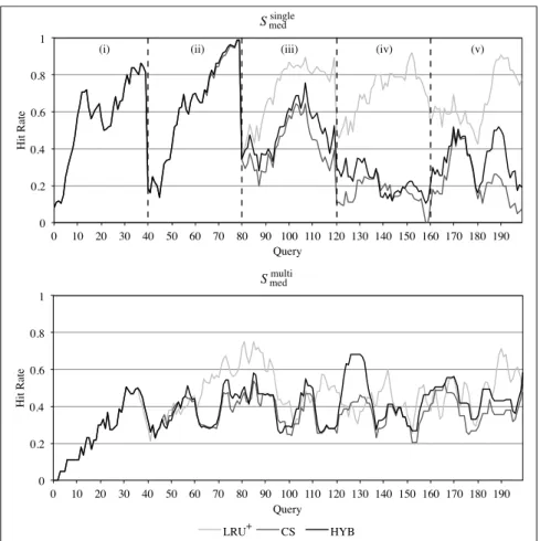
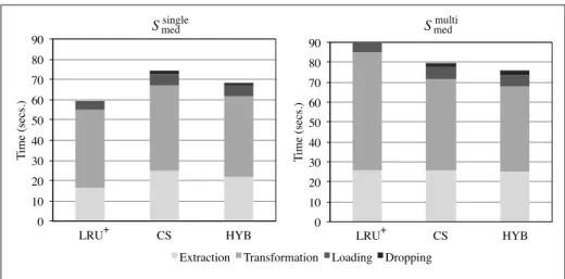
3.2.6.1 Dropping Policy Analysis . . . 40
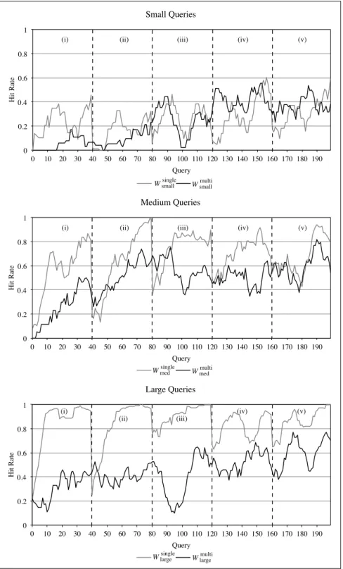
3.2.6.2 Reuse Analysis . . . 41
3.2.6.3 Comparison with Chunking . . . 43
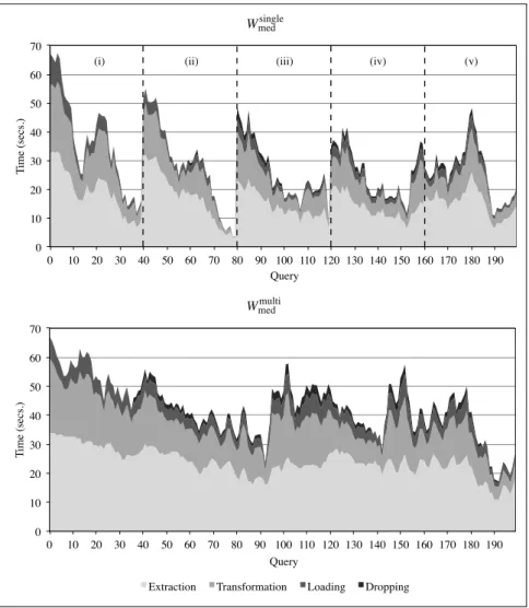
3.2.6.4 Efficiency Analysis . . . 47
3.2.6.5 Cost Function Analysis . . . 47
3.2.7 Wrapping up QETL . . . 48
3.3 Building Adaptive Cost Models for Web Services . . . 50
3.3.1 Related Literature . . . 51
3.3.1.1 QoS Prediction . . . 51
3.3.1.2 Cost Modeling with Machine Learning . . . 51
3.3.1.3 Database Histograms . . . 52
3.3.1.4 Active Learning . . . 53
3.3.2 Approach Overview . . . 53
3.3.3 Formal Framework . . . 54
3.3.4 Cost Model Management . . . 57
3.3.4.1 The SAIRT Algorithm . . . 57
3.3.4.2 Extending SAIRT with Multiple Linear Regression . . . . 58
3.3.5 Active Learning . . . 62
3.3.6 Experimental Results . . . 66
3.3.6.2 Active Learning Analysis . . . 71
3.3.7 Wrapping up Tiresias . . . 72
4 Compact Visualization of Multidimensional Data 73 4.1 Motivation and Outline . . . 74
4.2 Related Work . . . 76
4.3 Background on the Shrink Operator . . . 78
4.4 Optimization Techniques for the Shrink Operator . . . 82
4.4.1 Mathematical Formulation . . . 83 4.4.2 A Dual Ascent . . . 84 4.4.2.1 Parametric Relaxation . . . 85 4.4.2.2 Lagrangian Relaxation . . . 85 4.4.3 A Lagrangian Heuristic . . . 89 4.4.4 An Exact Method . . . 90 4.4.5 Computational Results . . . 91
4.4.5.1 Dual Ascent procedure . . . 92
4.4.5.2 Greedy and Lagrangian Heuristics . . . 98
4.4.5.3 Exact Method . . . 99
4.4.6 Wrapping up the new Shrink Implementations . . . 104
4.5 Multidimensional Shrink . . . 106
4.5.1 The Multidimensional Shrink Framework . . . 107
4.5.1.1 The Shrink Approximation . . . 112
4.5.1.2 The Reduction Problems . . . 114
4.5.1.3 Problem Search Space . . . 115
4.5.1.4 A Heuristic Approach . . . 116
4.5.2 Lazy Shrink Computation . . . 118
4.5.3 Eager Shrink Computation . . . 121
4.5.4 Experimental Results . . . 123
4.5.4.2 Efficiency Analysis . . . 128
4.5.5 Wrapping up Multidimensional Shrink . . . 130
5 Modeling of Unconventional Data Sources 133 5.1 Automating Multidimensional Modeling from Data Vaults . . . 134
5.1.1 Related Work . . . 134
5.1.2 Data Vault Basics . . . 136
5.1.3 Formal Background . . . 137
5.1.4 The Starry Vault Approach . . . 138
5.1.4.1 Hub-To-Hub FD Detection . . . 138
5.1.4.2 Md-Schema Discovery and Ranking . . . 141
5.1.4.3 Candidate Selection . . . 142
5.1.4.4 Md-Schema Construction . . . 142
5.1.4.5 Ranking . . . 144
5.1.4.6 Md-Schema Enrichment . . . 145
5.1.5 Wrapping up Starry Vault . . . 147
5.2 Multidimensional Modeling Over Sensor Data . . . 148
5.2.1 Related Literature . . . 149
5.2.2 Reference Architecture and Domain Model . . . 150
5.2.2.1 Functional Architecture of the Analytical System . . . 150
5.2.2.2 Domain Model . . . 153
5.2.3 Multidimensional Schemata . . . 155
5.2.4 Case Studies . . . 158
5.2.4.1 Air Quality Monitoring . . . 158
5.2.4.2 Requirements for Air Quality Monitoring . . . 159
5.2.4.3 Sensing Air Quality . . . 160
5.2.4.4 Warehousing Air Quality Data . . . 160
5.2.4.5 Landslides Risk Management . . . 162
5.2.4.7 Sensing Landslide Risk Data . . . 163 5.2.4.8 Warehousing Landslides Risk Data . . . 163 5.2.5 Wrapping up Sensor Data Modeling . . . 164
6 Conclusions 165
Acknowledgements
With the following few lines, I would like to thank all those people who helped and supported me during my PhD endeavours.
First, my sincere gratitude goes to Prof. Matteo Golfarelli and Prof. Stefano Rizzi, who not only taught me most of what I know about research, but also constantly motivated me to push forward.
In addition, I would like to thank Prof. Simon Dobson, who hosted me at the University of St Andrews, for all the valuable discussions and insights on sensor networks.
Moreover, I wish to thank all my colleagues and friends, with whom I shared many good laughs and who always have been there to help me.
Finally, above everyone else, I would like to thank my family, who patiently and steadily supported me, especially when I needed it the most. A big thank you to my two little nephews as well, who never failed to cheer me up.
Abstract
An OLAP analysis session is carried out as a sequence of OLAP operations applied to multidimensional cubes. At each step of a session, an operation is applied to the result of the previous step in an incremental fashion. Due to its simplicity and flexibility, OLAP is the most adopted paradigm used to explore the data stored in data warehouses. With the goal of expanding the fruition of OLAP analyses, in this thesis we touch several critical topics. We first present our contributions to deal with data extractions from service-oriented sources, which are nowadays used to provide access to many databases and analytic platforms. By addressing data extraction from these sources we make a step towards the integration of external databases into the data warehouse, thus providing richer data that can be analyzed through OLAP sessions. The second topic that we study is that of visualization of multidimensional data, which we exploit to enable OLAP on devices with limited screen and bandwidth capabilities (i.e., mobile devices). Finally, we propose solutions to obtain multidimensional schemata from unconventional sources (e.g., sensor networks), which are crucial to perform multidimensional analyses.
Chapter 1
Introduction
The term Business Intelligence (BI) refers to a set of processes and technologies that aim at gathering, transforming, and analyzing data with the end goal of obtaining useful insights for decision processes. Traditionally, at the core of a BI system lies a Data Warehouse (DW), which is a repository of integrated and consistent data modeled in a multidimensional fashion [1]. In the multidimensional model data are represented as cubes whose cells and edges respectively stand for events and analysis dimensions. Moreover, each cell is described by a set of measures (e.g., total income) and on top of each dimension is built a hierarchy that defines different levels of aggregation of the data.
Among the many techniques available to analyze the data stored in a DW, the most widespread isOn-Line Analytical Processing (OLAP). An OLAP analysis session is carried out as a sequence of OLAP operations (i.e., roll-up, drill-down, slice & dice, and pivoting) applied to multidimensional cubes. More precisely, at each step of the session, an operation is applied to the result of the previous step. This incremental approach coupled with the intuitive multidimensional model enables users with very limited IT expertise to carry out both explorative analyses and reporting duties. Due to its simplicity and flexibility, OLAP has been a staple technology of BI since its inception and still exists alongside the more sophisticated approaches offered by data mining techniques.
Although OLAP itself has not undergone significant changes, over the years the scope of the analyses in which it is used has been drastically expanding. Indeed, decision makers have started to incorporate more and more data that are not typically stored in corporate databases. For instance this is the case for social business intelligence [2], in which relevant data are fetched from the web in the form of user-generated content made available in forums, blogs, social networks, and the like; or it is the case for scientific applications where huge datasets (e.g., containing genomic data [3]) are shared worldwide and publicly available for research purposes. Besides, the fruition of BI is no more limited to desktop computers and it is now possible to carry out sophisticated analyses from mobile devices. While on the one hand these devices widen the fruition of BI technologies,
on the other they have some specific limitations, such as screen size and data bandwidth, that need to be taken into account by analysis tools. These limitations can bring new research opportunities and spur the creation novel approaches specifically tailored for mobile devices.
This work takes on the challenges and opportunities described above by focusing on bringing OLAP analyses to data sources and devices that traditionally do not support it. Specifically, the main issues tackled in this work that are critical to enable ubiquitous OLAP analyses are: (i) data extraction from service-oriented sources; (ii) compact visualization of multidimensional data; (iii) multidimensional modeling over unconventional data sources. The first issue is particularly relevant to extending the scope of traditional BI tools; indeed, many modern data sources are hidden behind service-based interfaces, which often have more restricted querying capabilities than traditional databases. The second issue is instead related to the fruition of OLAP analyses on mobile devices by allowing the users to tailor the visualization of multidimensional data based on their needs. Finally, the last issue has a similar goal to the first one (i.e., extending OLAP to new data sources), but instead of focusing on data extraction it tackles multidimensional modeling, which is crucial to enabling OLAP analyses.
In the following, the aforementioned research thematics will be briefly introduced empha-sizing our envisioned solutions and novel contributions. Specifically, Section 1.1 introduces the approaches designed to deal with service-based data sources, Section 1.2 presents our novel techniques for data visualization and, finally, Section 1.3 shows the results achieved related to multidimensional modeling. The rest of the thesis is structured as follows: Chapter 2 introduces the required background concepts; Chapters 3, 4, and 5 present in detail our novel contributions (introduced below); lastly, Chapter 6 draws the conclusions and sets the direction of potential future work.
1.1
Service-Oriented Data Sources
The contribution related to service-oriented data sources is twofold: the first part is an on-demand ETL framework especially tailored for non-owned data sources, while the second one is a technique to automatically build adaptive cost models for web services. Noticeably, the second contribution can sit on-top of the first one to enhance the optimization of data extractions. Indeed, each time an extraction is required, the proposed on-demand ETL approach has to find the best set of queries to issue to the data source that minimizes the cost of the operation (e.g., time). One of the key issues in this optimization problem is building a cost model that allows to predict the cost of a given query.
1.1.1
On-Demand ETL
In traditional OLAP systems, the ETL process loads all available data in the data warehouse before users start querying them. In some cases, this may be either inconvenient (because data are supplied from a provider for a fee) or unfeasible (because of their size);
on the other hand, directly launching each analysis query on source data would not enable data reuse, leading to poor performance and high costs. The alternative investigated here is that of fetching and storing data on-demand, i.e., as they are needed during the analysis process. In this direction we propose the Query-Extract-Transform-Load (QETL) paradigm to feed a multidimensional cube; the idea is to fetch facts from the source data provider, load them into the cube only when they are needed to answer some OLAP query, and drop them when some free space is needed to load other facts. Remarkably, QETL includes an optimization step to cheaply extract the required data based on the specific features of the data provider.
In greater detail, our novel contributions related to on-demand ETL are:
We introduce an abstraction calleddicefor compactly representing the facts available in a cube at each time, and we show how dice can be used to efficiently determine the facts missing to answer an OLAP query.
We present a heuristic algorithm that, given the missing facts and considering the features of the source data provider, finds the cheapest set of extractions that the ETL can carry out to fetch the data required.
We discuss the result of a set of experimental tests, performed using a ROLAP architecture, aimed at evaluating QETL from both points of view of efficiency and effectiveness and at comparing it with a previous approach in the literature.
1.1.2
Cost Models for Web Services
Delivering accurate estimates of query costs in web services is important in different contexts, e.g., to measure their Quality of Service. However, building a reliable cost model is difficult as (i) a web service is a black box often hiding a complex computation, (ii) a call to the same service can yield completely different costs by simply changing a parameter value, and (iii) execution costs can drift with time. We propose Tiresias, an approach that, given a web service exposing an interface with a fixed number of parameters, initializes and actively adapts a model to accurately predict query costs. The cost model is represented by a regression tree trained through two interleaved querying cycles: a passive one, where the costs measured for user-generated queries are used to update the tree, and an active one, where the service is probed through system-generated queries to cope with drifts in the cost function.
Overall, the main contributions are:
An architectural framework for deriving cost models of web services using their public interfaces only.
An extension of the SAIRT algorithm [4] that incorporates multiple linear regression models with the result of improving the overall accuracy while keeping training costs compatible with the requirements demanded by streaming applications.
An active learning algorithm that initializes the cost model and dynamically adjusts it in case of function drift.
A set of experimental tests performed on both real and synthetic datasets to evaluate Tiresias in terms of efficiency and effectiveness.
1.2
Visualization of Multidimensional Data
To cope with the problem of information flooding and with the limitations of mobile devices (i.e., screen’s size and data bandwidth), Golfarelli et al. [5] presented the shrink operator, which is aimed at balancing precision and size when visualizing multidimensional cubes via pivot tables. This operator can be applied during an OLAP session to the cube resulting from a query to decrease its size while controlling the approximation introduced. The idea is to fuse similar facts together and replace them with a single representative fact (computed as their average), respecting the bounds posed by dimension hierarchies. However, the implementation of shrink presented in [5] can operate on a single dimension at time. Furthermore, the algorithms presented, while correct, still have margin of improvement. Going in the direction of enhancing the shrink operator, in this work we present new algorithms for the mono-dimensional (both heuristic and exact) and a multidimensional generalization.
1.2.1
Optimization Techniques for the Shrink Operator
We propose a model to optimize the implementation of the shrink operation, which considers two possible problem types. The first type minimizes the loss of precision ensuring that the resulting data do not exceed the maximum size allowed. The second one minimizes the size of the resulting data ensuring that the loss of precision does not exceed a given maximum value. We model both problems as a set partitioning with a side constraint, which we solve with:
An original formulation of the problem as a set partitioning problem with side constraints.
An heuristic method based on dual ascent procedure that exploit pricing and Lagrangian relaxation.
An exact method which solves the problem starting from the dual solution found by the dual ascent procedure.
1.2.2
Multidimensional Shrink
Since the original shrink operation [5] can only be applied to one dimension (i.e., reduces a cube along one dimension), to improve its efficacy, we propose a multi-dimensional generalization where facts are fused along multiple dimensions. Multi-dimensional shrink comes in two flavors: lazyandeager, where the bounds posed by hierarchies are respectively weaker and stricter. Greedy algorithms based on agglomerative clustering are presented for both lazy and eager shrink, and experimentally evaluated in terms of efficiency and effectiveness.
The proposed contributions are the following ones:
The formalization of the shrink framework, including the computation of the shrink approximation, is generalized from the mono- to the multi-dimensional case. Two different forms of the hierarchy compliance constraints are defined (lazy and
eager).
The size of the search space for computing both lazy and eager shrink is characterized, and greedy algorithms are proposed.
The approach is evaluated in terms of efficiency and effectiveness, also in comparison to those achieved by traditional roll-up and mono-dimensional shrink.
1.3
Multidimensional Modeling
Multidimensional modeling is required to enable OLAP analyses, however it is often a non-trivial task to obtain a proper schema for a given domain. For this reason we present: an automatic approach to obtain multidimensional schemata specifically tailored for data vaults [6]; and a set of manually designed schemata for sensor data.
1.3.1
Automatic Multidimensional Modeling for Data Vaults
The data vault model natively supports data and schema evolution, so it is often adopted to create operational data stores. However, it can hardly be directly used for OLAP
querying. We propose an approach called Starry Vault for finding a multidimensional structure in data vaults. Starry Vault builds on the specific features of the data vault model to automate multidimensional modeling, and uses approximate functional dependencies to discover out of data the information necessary to infer the structure of multidimensional hierarchies. The manual intervention by the user is limited to some editing of the resulting multidimensional schemata, which makes the overall process simple and quick enough to be compatible with the situational analysis needs of a data scientist.
1.3.2
Multidimensional Modeling Over Sensor Data
Due to the rapid growth of the Internet of Things [7], sensors are more and more ubiquitous and are quickly becoming one of the major sources of data. While these data are usually well exploited for real-time monitoring tasks, the knowledge to properly handle them in an integrated and long-term fashion is still missing. To fill this gap we propose the following contributions:
We present a functional architecture to support both real-time and off-line analyses. We introduce a set of multidimensional schemata covering the main requirements
typical of systems that deal with sensor data.
Chapter 2
Background Concepts
In this chapter we define some of the basic concepts used throughout the rest of this work. We start by giving an informal presentation of OLAP analysis and ETL, respectively in Section 2.1 and 2.2. We then close with Section 2.3, which defines the shared formal framework that will be used to support our novel contributions. Please, notice that both Section 2.1 and Section 2.2 are not meant to be in-depth presentations, indeed, they are meant to serve as an introduction for the novice reader.
2.1
OLAP Analysis
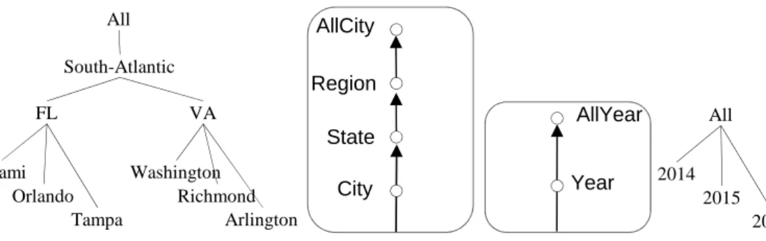
In the context of BI the main paradigm used for modeling data is the multidimensional one. As shown in Figure 2.1, in a multidimensional cube events to be analyzed (e.g., census outcomes) are associated with multidimensional cube cells, while cube edges stand for analysis dimensions (e.g., RESIDENCE,TIME,OCCUPATION). For each cube cell is given a value for each measure describing the event (e.g., citizen incomes, number of children). On top of each dimension is built a hierarchy that defines groupings of its values. An example of cube is shown in Figure 2.1, while an example of hierarchies associated to dimensions are shown in Figure 2.2.
TIME RESIDENCE OCCUPATION 2016 clerk Miami 15
Figure 2.1: An example of a three dimensional cube
All South-Atlantic FL VA Miami Orlando Tampa Washington Richmond Arlington All 2014 2015 2016 City State Region AllCity Year AllYear RESIDENCE TIME
Figure 2.2: Roll-up orders and functions for two hierarchies in the CENSUS schema
Multidimensional cubes are queried through OLAP (On-Line Analytical Processing) queries, which allow users to interactively navigate the data without requiring advanced IT skills. An OLAP session is a navigation path composed by a sequence of queries. At each step of a session, the user can apply an OLAP operator to the result obtained from the previous
(a) Roll-up (b) Drill-down (c) Slice-and-dice
(d) Pivoting (e) Drill-across
Figure 2.3: Visual representation of the OLAP operators
one. The most common OLAP operators are roll-up, drill-down, slice-and-dice,pivoting, drill-across, and drill-through.
The roll-up operator aggregates data, thus reducing the level of detail (see Figure 2.3a). For instance, when applying a roll-op from City toState, the result will be a set of facts aggregated by State(e.g., the average income for each state).
As shown in Figure 2.3b, the drill-down operator yields the opposite result of roll-op, hence it increases the level of detail of the data (e.g., from Stateto City).
Slice-and-dice (see Figure 2.3c) reduces the number of visualized values by means of filtering (e.g., City = Bologna).
Pivoting (see Figure 2.3d) causes a change in layouts, aiming at analyzing a group of data from a different viewpoint.
Through the drill-across operator (see Figure 2.3b) it is possible to link the cells of different cubes to get a broader view of the data in the DW.
The drill-through operator switches from multidimensional aggregated data to the data stored in operational data sources. This operator is rarely implemented by BI tools; indeed, the drill-through function of commercial tools is often a simple view of the data in the DW at the finest granularity.
Year 2010 2011 2012 Cit y Miami 47 45 50 Orlando 44 43 52 Tampa 39 50 41 Washington 47 45 51 Richmond 43 46 49 Arlington — 47 52
Figure 2.4: A simple pivot table showing data per City and Year
The results obtained during an OLAP analysis are usually visualized either through charts (e.g., bar charts) or through pivot tables (as shown in Figure 2.4). While charts are more effective at summarizing big amounts of data, they might become too complex to understand when dealing with more than two dimensions. On the other hand, while pivot tables are simple and more flexible than charts, their readability quickly declines as the quantity of data to visualize rises.
To close this brief introduction on OLAP analysis, we remark that commercial analysis tools (e.g. Tableau 1) are nowadays trying to seamlessly include the OLAP exploration style of analysis with more advanced techniques (e.g., clustering, regression analysis, etc.) Furthermore, modern tools often mask the implementation of these operators behind clever interfaces that allow to execute complex operations with minimal effort.
2.2
ETL
The Extract, Transform, and Load (ETL) process is in charge of extracting data from operational data sources, enforcing quality and consistency standards (so that data coming from different sources can be integrated) and, finally, feeding the DW. Traditionally, this process is executed periodically (e.g., daily) in a batch fashion. The frequency of the ETL must be carefully chosen: a more frequent ETL allows for up-to-date data but at the cost of a heavier burden placed on operational sources; on the other hand, a less frequent ETL might result in stale data but has a smaller impact on data sources.
In the following we describe the main phases of the ETL process.
Extraction: it includes the extraction of data from the operational sources. The extraction can be eitherstatic or incremental. A static extraction is used to populate
the DW from scratch; an incremental extraction is instead used to update the DW depending on the changes occurred in the operational data.
Transformation: this phase is in charge of cleaning and preparing the data to be fed to the DW. The cleansing part of this phase includes all those operations that aim at improving the data quality and consistency. For instance, the operational data might contain duplicate values, missing data, impossible values, etc. After all these issues have been addressed, the data need to be integrated and transformed into a format that is more suitable for analytic queries; for example, denormalizations of the schemata are often introduced to improve performances at query time.
Loading: it is the last step of the ETL process. Similarly to the extraction phase, it can be carried out in two ways: refresh and update. In the former case, the DW is completely rewritten; in the latter one, only those changes applied to source data are added to the DW.
While traditionally the ETL process is periodically executed in a batch fashion, nowadays business users demand approaches that are more agile and flexible. As discussed in literature [8], ETL processes and DW architectures need to evolve to manage the growing data heterogeneity (e.g., sensor data) and strict freshness requirements (e.g., near real-time scenarios). Section 3.2 will treat this topic in greater detail and present our novel approach to on-demand ETL.
2.3
Formal Framework
In this section we present the main definitions shared by the approaches presented in the following chapters.
Definition 1 (Multidimensional Schema) An n-dimensional schema (or, briefly, a schema) M is a couple of
a finite set of hierarchies, H th1, . . . , hnu, each characterized by a set Li of levels
and a roll-up total order i of Li. Each level l is defined over a categorical domain
of members, Domplq. The domain of the top level of each hierarchy has a single All member. Apices will be used to denote the hierarchy each level belongs to; besides, the indexes of levels will be ordered according to their roll-up order: li1 i li2 i . . ..
a family of roll-up functionsincluding, for each pair of adjacent levels lij and lij 1, a function RUl i j 1 li j :Dompli
jq ÑDomplji 1q that associates each member in Domplijq to
Let two levelslji, lik PLi with j ¤k be given. Given member mPDompljiq, we denote with
Rollkpmq the member ofli
k recursively defined as follows:
Rollkpmq $ & % m , if kj RUl i k li k1p Rollk1pmqq , if k¡j
We say that m rolls-up to Rollkpmq. Conversely, given a set of members M Domplkiq, we denote with DrilljpMq the set of members of lji that roll-up to a member inM.
Example 1 IPUMS is a public database storing census data [9]. As a working example we will use a simplified form of its CENSUS multidimensional schema based on two hierarchies, namely RESIDENCE and TIME. Within RESIDENCE it is City RESIDENCE State, and
MiamiP DompCityq rolls-up to FL PDompStateq and toSouthAtlanticPDompRegionq (roll-up orders and functions are shown in Figure 2.2).
The possible ways to aggregate data are captured by the following definition.
Definition 2 (Group-by) A group-by of schema M is an element GP L1. . .Ln.
A coordinate of G xl1, . . . , lny is an element dPDompl1q . . .Domplnq (which, with a slight abuse of formalism, we will denote with dPG).
Example 2 Some examples of group-by on the CENSUS schema are G1 xCity, Yeary
and G2 xRegion, Yeary. A coordinate of G1 is xMiami, 2012y.
All facts in a cube are characterized by the same group-byG, that defines their aggregation level, as well as by a coordinate of G and by a numerical value v; this can be formalized as follows:
Definition 3 (Cube) A cube at group-by G is a function C that maps each coordinate of G either to a numerical value called measure or to N U LL. Each couple xd, Cpdqy with Cpdq N U LL is called a fact of C.
The reason for using N U LLs is that cubes are normally sparse, i.e., some facts are missing. An example of missing fact is the one for the Arlington city and year 2010 in Figure 2.4. Example 3 Two examples of facts of CENSUS are
xxMiami,2012y,50y xxOrlando, 2011y,43y
The measure in this case quantifies the average income of citizens. A possible cube at G1
Chapter 3
Extracting Data from
Service-Oriented Sources
In this chapter we describe our novel contributions related to service-oriented data sources. After a brief introduction (see Section 3.1), we proceed to present QETL (see Section 3.2), which is an on-demand ETL framework designed to cope with those scenarios where loading all available data might be either inconvenient, or even unfeasible because of their size and cost of access (i.e., data for a fee). The idea behind QETL is that of fetching facts from the source data provider, loading them into the cube only when they are needed to answer some OLAP query, and dropping them when some free space is needed to load other facts.
The other approach presented in this chapter is Tiresias (see Section 3.3), whose aim is that of automatically building cost models for web services. Delivering accurate estimates of query costs in web services is important in different context, e.g., to measure their Quality of Service. However, building a reliable cost model is difficult as (i) a web service is a black box often hiding a complex computation, (ii) a call to the same service can yield completely different costs by simply changing a parameter value, and (iii) execution costs can drift with time. Given a web service exposing an interface with a fixed number of parameters, Tiresias initializes and actively adapts a model to accurately predict query costs.
3.1
Service-Oriented Data Sources and BI
Data warehouses (DWs) have been used for almost two decades in company settings to store information useful for decision making. Most of this information is typically gathered from corporate operational databases using an ETL (Extract-Transform-Load) process that extracts relevant data, transforms them into multidimensional form, and loads them into the DW in the form of cubes, to be later analyzed by means of reporting and OLAP tools. Traditionally, ETL is performed on a periodic basis by fast bulk-loading techniques during a time window in which the DW is in a quiescent state, i.e., is not queried by end-users. This means that, at query time, the information available has already been loaded in its entirety into the cubes.
Over the last few years, the scope of the analyses carried out by decision makers has been increasing in size to encompass a relevant quantity of data that are not necessarily stored in corporate databases. For instance this is the case for social business intelligence, in which relevant data are fetched from the web in the form of user-generated content made available in forums, blogs, social networks, and the like; or it is the case for scientific applications where huge datasets (e.g., containing genomic data) are shared worldwide and publicly available for research purposes. These data are often accessible through web services, whose functionalities range from simply granting the access to data stored on a DBMS, to running complex analyses on raw data aimed at returning valuable information. In this context, our twofold contribution is presented in detail in Section 3.2 and 3.3.
In Section 3.2 we define an on-demand ETL framework that allows the user promptly extract data from web services and load them in the DW for future reuse. Indeed, in many cases loading all available data into the DW cubes at ETL time may be either inconvenient (because data are supplied from a provider for a fee) or unfeasible (because of their size); on the other hand, directly launching each analysis query on source data would not enable data reuse, thus leading to poor performance and high costs. The QETL approach works as follows: given a user query, QETL extracts the required data and, if needed, drops already loaded facts to make room for the new query. Furthermore, to reduce the ETL costs, QETL includes an optimization step to cheaply extract the required data based on the specific features of the data provider.
In Section 3.3 we present instead an approach to automatically build cost models for web services. In several cases, single services must be composed so that information from different sources can be integrated and complex workflows can be obtained. When multiple service compositions are feasible, the choice is often based on the Quality of Service (QoS). An important indicator of QoS for web services is the cost (typically, the execution time) for answering a query. Unfortunately, obtaining good estimates is often difficult, especially in the case of services that offer complex
analyt-ics, where a call to the same interface can trigger completely different computations by simply changing a set of parameter values. To automatically build a cost model from such services, Tiresias employs regression trees trained through two interleaved querying cycles: a passive one, where the costs measured for user-generated queries are used to update the tree, and an active one, where the service is probed through system-generated queries to cope with drifts in the cost function.
Noticeably, the latter contribution can be stacked on top of the former to enhance it. The statistics obtained through the cost models of the queried services can in fact be used to optimize the extractions issued by the on-demand ETL.
3.2
On-Demand ETL from Non-Owned Data Sources
As introduced above, traditional batch ETL approaches can be inconvenient or even unfeasible in many cases. The alternative investigated here is that of incrementally fetching and storing data on-demand, i.e., as they are needed during the analysis process. In greater detail, this on-demand approach can be especially useful in the following main application scenarios:
When source data are supplied for a fee by one or more data providers, on-demand ETL enables exactly extracting the data that are actually necessary and allowing reuse of that data by several users at different times, thus reducing the overall costs of analyses.
In scientific settings, the amount of possibly useful data shared by all the specialized repositories available worldwide can be intractable [3], so on-demand ETL can effectively cut the bootstrapping time by allowing incremental extraction and reuse of data.
In a situational business intelligence scenario, the decision process is empowered with open/linked data that have a narrow focus on a specific business problem and, typically, a short lifespan for a small group of users [10]; in this context, on-demand ETL is a key for fetching, at each time, the relevant data needed for each specific analysis.
More and more companies are using so-called data lakes to “park” huge volumes of low-quality and heterogeneous data in their native format until they are needed; in this setting, the complexity of cleaning and transforming these data to integrate them in the decision process discourages users from adopting a traditional batch ETL approach, making an on-demand approach preferable. In the latter scenario the data lake would be treated as any other data source that feeds the DW, and ETL operations would be applied only to the data that are required by analyses.
Before presenting the outline and main contributions of this work, we provide a description of the use case (that will serve as motivating example) followed by the basics of the formal framework.
3.2.1
Motivating Example
The GenData 2020 project aims at managing genomic data through an integrated data model, expressing the various features that are embedded in the produced bio-molecular data and in their correlated phenotypic data. This goal is achieved by enabling viewing, searching, querying, and analyzing over a worldwide-available collection of shared genomic
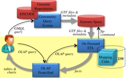
On-Demand ETL OLAP query GMQL query Genometric Query System Mapping Cube OLAP Front-End Genome Space ENCODE OLAP query Genomic Repositories facts tables & charts ftp command GTF files & metadata GTF files & metadata DW
Figure 3.1: Analysis of genomic mappings in the GenData 2020 framework
data. One of the analysis services envisioned within this framework is the multi-resolution analysis of the mappings between regions (i.e., segments of the genome) andsamples (i.e., sets of regions and correlated metadata resulting from an experiment) [3, 11]. As sketched in Figure 3.1, these mappings are computed by issuing a query in an ad-hoc language called GMQL (GenoMetric Query Language) against some repositories of genomic data such as ENCODE.1 The query output, called genome space, comes in the form of a set of
GTF (Gene Transfer Format,http://genome.ucsc.edu) files and related metadata, and due to its huge size is stored using the Hadoop platform.
OLAP-like queries are a valuable tool for biologists [3] because they enable multi-resolution analyses based on standard hierarchies of concepts; besides, they are preferred to traditional browser-based approaches because they enable a far more flexible and user-driven navigation of data. Unfortunately, the genome space generated by most biologically-relevant queries is too large to enable a traditional ETL process to load it into a multidimensional cube in a DW for OLAP analyses. This is where on-demand ETL comes into play. When a user formulates an OLAP queryq, the front-end sends it to the on-demand ETL component for processing. If all the multidimensional data (called factsfrom now on, and including both the actual mappings and the correlated dimensional data about the involved regions and samples) necessary to answerq are already present in the mapping cube (i.e., they have been previously loaded), they are sent to the front-end and shown to the user. Otherwise, the genome space is accessed via FTP to fetch all the missing data, that are then transformed and loaded onto the mapping cube, so thatq can be answered. Of course, from time to time, some facts used for past queries must be dropped from the cube to make room for the facts needed for new queries.
1ENCODE, theEncyclopedia of DNA Elements, is a public repository (accessible via FTP) created and
maintained by the US National Human Genome Research Institute to identify and describe the regions of the 3 billions base-pair human genome that are important for different kinds of functions [12].
MAPPING Experiment Chromosome Count Sample Tissue Region IN PU T R EF ER EN C E
Figure 3.2: The MAPPINGschema (the two Alltop levels are not shown)
All Spleen Exp1 Exp2 S11 S21 S31 S12 S22 S32 All Ch1 Ch2 R11 R21 R12 R22 Experiment Chromosome Sample Tissue Region IN PU T R EF ER EN C E
Figure 3.3: Fictitious roll-up functions for the INPUT and theREFERENCE hierarchies
3.2.2
Formal Background
In this section we recall the basic formal setting introduced in Section 2.3, adapting the presented definitions and enriching them with examples related to our case-study. For simplicity, we will consider hierarchies without branches, i.e., consisting of chains of levels, and facts with a single measure; see Section 3.2.5.7 for a discussion of how to deal with branched hierarchies and multiple measures.
We start by simplifying the notation of roll-up functions; indeed, as we only need to roll-up from members at the finest levels, i.e., m P l1i, we will simplify the roll-up definition as RollU plik :Dompli
1q ÑDomplkiq for each level lki.
Example 4 As a working example we will use a simplified form, shown in Figure 3.2, of the MAPPING schema adopted in GenData 2020 for OLAP analysis of mappings (the complete schema is shown in [11]). The schema includes two dimensions, namely INPUT
and REFERENCE. Within the INPUT hierarchy, Sample INPUTExperiment INPUT Tissue,
RollU pExperimentpS21q Exp1, and RollU pTissuepS21q Spleen (see Figure 3.3).
We also reuse Definition 2 and 3, which respectively describe the concept of group-by and cube.
G1 xSample,Chromosomey, and G2 xTissue,Regiony. A coordinate of G1 isxS21,Ch2y.
Example 6 Two examples of facts of MAPPINGarexxS21,R22y,2yandxxS21,Ch2y,900y. The measure in this case counts the number of regions of each input sample that overlap with each reference region.
3.2.3
Contribution and Outline
In this work we present QETL (Query-Extract-Transform-Load), an approach to on-demand ETL for feeding a multidimensional cube in scenarios where batch-loading the whole cube before query-time is either unfeasible (e.g., for space reasons) or inconvenient (e.g., for time or cost reasons). In QETL, facts are incrementally fetched from the source data provider and loaded into the cube only when they are needed to answer some OLAP query, to be possibly later dropped when they can be considered obsolete or when some free space is needed to load other facts. We remark that, in this context, with the term fact we mean not only the core multidimensional data (i.e., the measure values for a given multidimensional coordinate), but also the correlated dimensional data (i.e., the coordinate values and the corresponding hierarchy values). This means that, with reference to a classical star schema implementation, QETL works by loading/dropping tuples of fact tables and dimension tables at the same time.
The reason for storing the loaded facts into the cube (rather than simply using them to answer the OLAP query on-the-fly) is twofold. In scenarios where several users are concurrently analyzing the same cube, this caching-like mechanism encourages data reuse and cuts the cost for re-fetching the same facts twice or more. On the other hand, even when facts are mostly accessed by a single user (as in the genomic example, because each user normally builds her own mappings using custom GMQL queries), caching the facts extracted is convenient because the queries expressed during an OLAP session normally tend to be contiguous in terms of the facts they require [13].
In [3, 11] we set a case for on-demand ETL in the context of genomics and described a general framework for analyzing genome data. In this work we propose a specific solution to on-demand ETL; in particular:
(i) We introduce an abstraction calleddicefor compactly representing the facts available in a cube at each time, and we show how dice can be used to efficiently determine the facts missing to answer an OLAP query.
(ii) We present a heuristic algorithm that, given the missing facts and considering the features of the source data provider, finds the cheapest set of extractions that the ETL can carry out to fetch the data required.
architecture, aimed at evaluating QETL from both points of view of efficiency and effectiveness and at comparing it with a previous approach in the literature.
The outline of the contribution is as follows. After surveying the related literature in Section 3.2.4, Section 3.2.5 describes QETL in detail, while Section 3.2.6 shows the results of the experimental tests we performed. Finally, in Section 3.2.7 we draw the conclusions.
3.2.4
Related Literature
Enabling OLAP-like analyses on data different from those stored in traditional corporate databases is one of the most pressing requirements from decision makers, data scientists, and researchers [14]. One of the barriers that must be broken to achieve this goal is the limitation of traditional ETL processes that are typically batch, heavy, and strongly oriented to corporate and structured data. This requirement has been discussed in several vision papers. Abell´o et al. [10] envision an architecture forsituational business intelligence and discuss the related research challenges emphasizing the need for data extractors capable of connecting to external data sources and rewriting queries on them. Morton et al. [15] push this concept further by defining a new type of analyst, the data enthusiast, who has very limited ICT skills but must be enabled to connect and query several different, and possibly unstructured, data sources.
The problem of loading external data into a DW is strictly related to the one of defining a multidimensional schema of these data. Several papers focus on the problem of automati-cally deriving a conceptual schema from non-conventional data sources such as linked data [16, 17], ontologies, and user-generated content [18]. Although some of them also propose a technique for semi-automatically deriving the ETL procedures that extract data from these sources [19] and for mapping the non-conventional sources onto a multidimensional schema [16, 17], none discusses on-demand loading and its optimization.
When users ask for strictly up-to-date data, a right-time DW is needed. This term is used to mean that changes in the real world are propagated to the DW in a timely fashion (not necessarily in real-time). In a right-time DW architecture [20] there are two components whose performance is crucial to assuring real-time or near-real-time processing of data: optimized ETL software and refreshing software. Logical optimization, focusing on restructuring ETL processes in order to minimize the cardinality of data flows, has been proposed by Simitsis et al. [21, 22]. In particular, [22] proposes a heuristic for searching the space of possible ETL graphs to find the most efficient execution. In [23] a new type of join, called MeshJoin is proposed for joining a fast update stream with a large disk-resident relation under the assumption of limited memory. Refreshing software is typically based on views and materialized views. The main issue here is to avoid inconsistencies on materialized views that are read and refreshed and, at the same time, are modified by operational transactions. There are a number of solutions that avoid this
inconsistency, based on (i) applying algorithms that compensate for out-of-date data [24], (ii) maintaining two versions of materialized views, where one version is being refreshed while the other is being read [25], or (iii) using additional data structures and transactions [26]. While the problem of delta-extraction (at each run of ETL, only the operational data updated/added since the last run are extracted) is obviously addressed in these works, no mention is made to on-demand ETL (i.e., to extracting facts as they are required by user queries).
Two approaches similar to ours are proposed by Kargin et al. [27] and Idreos at al. [14]. The first paper introduces lazy ETL, that delays ETL at query time. Since extraction and transformation are implemented as relational algebra operators, the applicability and expressiveness of the approach are quite limited; furthermore, cache management is left to the DBMS with no specific optimization. Similarly, Idreos at al. sketch a system capable of loading at query time portions of data involved in the current query and stored in external flat files. Like in [27], they envision a set of relational operators to be added to the current query to enable source data retrieval. The minimum portion of data to be loaded is a column value and no optimization of the data extraction process is proposed. None of the previous papers adopt a formal framework for describing the proposed solutions. Another interesting approach that delays ETL at query time isLenses [28, 29], a framework for pay-as-you-go data curation (e.g., entity resolution and schema matching) based on probabilistic query processing. While that work can be placed in the context of on-demand ETL, the problem definition is quite different from ours. Indeed, in QETL the ETL effort is reduced by focusing the extractions on the facts required by user queries and by leaning on data reuse; conversely, the Lenses approach provides approximate, probabilistic answers so that not all the queried data have to be processed. While QETL provides exact answers, the basic claim in Lenses is that the user might prefer an approximate but less expensive answer; for instance, this might be the case during exploratory analysis.
A neighboring research topic is that of data caching. Indeed, the whole DW can be considered as a cache because it avoids directly accessing operational data to answer OLAP queries. The interest in caching issues in the DW literature radically changes depending on the infrastructural level considered. Caching of the query results has been pioneered by the WATCHMAN cache manager [30], which uses two algorithms for (in-memory) cache replacement and cache admission. An ad-hoc profit metric has been devised considering, for each retrieved set of data, its average rate of reference, its size, and the execution cost of the corresponding query. Noticeably, our approach bears several similarities with semantic caching [31]. The idea behind semantic caching is that of compactly representing stored queries by means of semantic descriptions, which is especially useful in client-server settings to reduce network overhead. However, approaches like semantic caching cannot be directly applied whenever data sources have limited query capabilities (e.g., they do not offer a logical negation operator). Other studies try to address these limitations by proposing systems specifically tailored for keyword-based
queries [32] or, more in general, for web databases [33]. Finally, several papers address the topic of materialized views, whose underlying idea is that of caching aggregated data within the DW to reduce the aggregation cost at query-time (see [1] for a review). Less interest has been raised in the use of caching at the ETL level, for instance, in [34] Liu proposes to use caching to optimize ETL data flows. To the best of our knowledge, no one of these papers proposes the use of the cubes themselves as a cache for data sources that cannot fit the available space —which is one of the use cases for QETL.
Our approach is also related to chunking, an approach for partitioning a cube into sub-cubes called chunks [35, 36]. Like a dice in QETL, a chunk is formally defined as a set of elements of a multidimensional array; differently from dice, chunks have fixed size and shape. While in QETL the goal of the dice construct is to enable a fast computation of the facts required by a user query and still missing from the cube, chunking is normally aimed either at minimizing the reading times from disk in MOLAP implementations of DWs, or at separating dense areas of a cube from sparse areas in HOLAP (hybrid OLAP) implementations. To the best of our knowledge, the only approach that uses chunking to reduce the complexity of caching is the one by Deshpande et al. [35]; though they need to find which chunks overlap with each multidimensional query, the computation of a “chunk difference” is rather simple: since all chunks have the same shape and size, the system simply needs to check which chunks overlap with the query and which chunks are already stored in the cache. Using chunking for our QETL approach has several drawbacks, all tied to the fact that chunking requires to specify both the number and shape of chunks beforehand: (i) a chunk envelope might not fit perfectly a given query, thus containing data that are not actually necessary; (ii) in our scenario, where some dimensional data are incrementally loaded, it might not be possible to define homogeneous chunks; and (iii) even if some algorithms to find the optimal number and shape of chunks exist [36],
the solutions obtained can significantly depend on the type of workload. Despite these potential drawbacks, in Section 3.2.6.3 we experimentally compare the chunking approach with ours.
Overall, among the above-mentioned approaches, those that bear most similarity with ours are those by Kargin et al. [27] and by Ren et al. [31]. However, to address the query trimming problem (i.e., given two overlapping queries, determine the tuples contained in one but not in the other), both these approaches resort to the full expressiveness of relational algebra —which is often missing in data sources with limited query capabilities. Conversely, the querying expressiveness required by QETL is just that of selection on attributes —which is normally available in data sources. Besides, in lazy ETL [27] data extraction is not optimized when data sources with multiple interfaces are present, while with QETL we introduce a heuristics to minimize the cost of the issued queries. Finally, while the dice construct resembles chunking [35], the former overcomes many limitations of the latter by defining a more flexible and accurate envelope to represent multidimensional data.
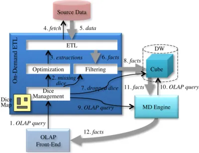
MD Engine Source Data 10. OLAP query 4. fetch 5. data OLAP Front-End Cube Optimization Filtering ETL 1. OLAP query 12. facts 9. OLAP query 2. missing dice 3. extractions 6. facts O n-D em and ETL 8. facts 11. facts Dice Management Dice Map 7. dropped dice DW
Figure 3.4: Functional architecture for on-demand ETL; black arrows represent function calls, while gray arrows indicate data flows
3.2.5
The QETL Approach
A functional view of the QETL process is shown in Figure 3.4, and its components are explained below. Though QETL can operate on multiple cubes, for simplicity we show a single cube. The abstraction we use to compactly represent the facts currently stored in the cube, those required to answer an OLAP query, those missing, and those to be requested to the source data provider through the ETL is called dice and is formally defined in Section 3.2.5.1; intuitively, a dice is a multidimensional interval of coordinates that determines a set of facts.
Thedice managementprocess takes an OLAP query q and checks, using a map of the dice currently available in the cube (dice map), ifq can be immediately answered or some facts are missing. In the first case, q is sent to the multidimensional engine for processing. In the second case, the difference between the dice required by q and the available dice is computed in terms of a set of missing dice and handed to the optimization process. This process is also in charge of choosing the dice to be dropped from the cube when some room is needed. Of course, when QETL operates on multiple cubes, each of them requires a separate dice map.
ETL: this is a traditional ETL process that offers an interface consisting of a set of (extraction) services. To comply with the limitations often posed by the source data provider and by its query language, we assume that each service supports selection predicates on one or more levels (e.g., it might support selections on Tissue and
Chromosome) and is capable of returning the set of facts corresponding to a single
into a query on the source data provider, fetches the required data, and transforms them into multidimensional form. The ETL has a model for estimating the cost of each call to a service, based in general on both the cost for data fetching and those for their transformation.
The optimizationprocess knows the interface offered by the ETL and the cost for each service call as exposed by the ETL. Based on this information, it determines a set of extractions that cover all the missing dice and has total minimum cost. Each extraction entails a call to a service.
Since the interface exposed by the source data provider does not necessarily allow full querying expressiveness, the facts fetched at each time may be a superset of those actually needed. The filteringprocess filters them before loading them into the cube; then it sends the set of loaded dice to the dice management process that updates the dice map accordingly.
With reference to the numbered arrows in Figure 3.4, the workflow of QETL can be schematically described as follows.
0. The user visually formulates an OLAP query on the OLAP front-end.
1. The OLAP front-end sends the query (e.g., in MDX format) to dice management. If some facts are missing: 2. Dice management determines the set of missing dice and transmits them to optimization and filtering. 3. Optimization determines a set of optimal extractions and calls the ETL service accordingly.
4. ETL sends a fetching query to the source data provider. 5. The source data provider returns the required data.
6. ETL puts the data in multidimensional form and sends the resulting facts to filtering. If there is not enough room in the cube:
7. Dice management chooses the dice to be dropped from the cube. 8. Filtering loads the filtered facts into the cube.
9. Dice management sends the query to the MD engine. 10. The MD engine executes the query on the cube. 11. The query answer is returned to the MD engine.
12. The MD engine returns the query answer to the OLAP front-end.
In the following, we proceed to describe in greater detail the dice management, optimization, and filtering processes. As to ETL we emphasize that, in our Query-Extract-Transform-Load paradigm, each user query triggers not only an extraction and a loading, but also a transformation. However, the focus of this work is on incremental extraction and loading, so we will not specifically discuss the complexities of transformation (though in our experimental tests we will consider and single out the cost for transformation as well).
3.2.5.1 Query and Extraction Model
An OLAP query is normally defined by a group-by G and some selection predicates expressed on levels. To start simple, here we assume that facts are extracted and loaded into the cube only at their finest granularity, to be then aggregated byGby the multidimensional engine (in Section 3.2.5.7 we will discuss the implications of extracting and storing facts at different group-by’s). For this reason, G is not relevant from the point of view of on-demand ETL, and we can simply represent a query q as a set of multidimensional intervals —those induced through the roll-up functions on the domains of the finest levels l1
1, . . . ln1, etc. by the selection predicates of q— that determine the coordinates of the facts
to be returned to the user. The abstraction we use to this end is calleddice and defined below.
Definition 4 (Range and Dice) Arangeriof levelli
1is an interval of memberspm1, m2q
such that m1, m2 PDompli
1q and m1 ¤m2. A dice d is an n-dimensional interval of
coor-dinates, dni1ri where ri is a range of li1 for i1, . . . , n.
Working with ranges requires that a total order is defined on the members of each levelli
1.
To define such order we observe that, in several OLAP front-ends, the default behavior when a user clicks on a row/column of a pivot table (corresponding to a member of a level) is to disaggregate the measure values for that row/column into its components, which in OLAP terms means slicing and drilling down [13]. For instance, starting from a report showing mappings per tissue and chromosome, clicking on member Spleen would trigger a query showing mappings for experiments Exp1 and Exp2, while clicking on Ch1 would trigger a query showing mappings for regions R11 and R21. Normally, within each group, members are alphabetically sorted. For this reason, to define ranges and dice we will adopt ahierarchy-based lexicographic order, i.e., one in which the members that roll-up to the same member are lexicographically ordered.
From the topological point of view, two dicedandd1 are either disjoint (dkd1), overlapping (dd1), or one of them is included in the other (dd1). Of course, the exact relationship between two dice depends on whether each range in each dice is left-open/closed and right-open/closed; notice that, to avoid unnecessary notational complexity, we purposefully omitted these details from Definition 4. If you consider the example in Figure 3.5, with d pS11,S31qpR11,R14q,d1 pS22,S23qpR44,R45q, andd2 pS31,S43qpR22,R45q, it is alwaysdkd1, but the other relationships depend on the range closeness. Specifically, if d is right-closed and d2 is left-closed on the first dimension, then d d2, otherwise dkd2. Similarly it can be either d1 d2 (when d1 is right-closed andd2 is right-open on the second dimension) or d1 d2 (in all other cases).
Definition 5 (OLAP Query) An OLAP query is defined as a set Q of dice that repre-sent the coordinates of the facts to be returned.
d d' d" S11 S21 S31 S12 S22 S32 S13 S23 S33 S43 R11 R21 R12 R22 R13 R23 R33 R43 R14 R24 R34 R44 R15 R25 R35 R45
Figure 3.5: Topological relationships between three dice
Example 7 A dice of our MAPPING schema is d pS11,S12q pR22,R22q. Adopting the hierarchy-based lexicographic order for the domains of both regions and chromosomes (like in Figure 3.3), this dice includes 41 coordinates. The query asking for the number of mappings between samples of tissue Spleen and regions of chromosome Ch2 is defined by Q tpS11,S32q pR12,R22qu (which includes 62 coordinates).
Like for OLAP queries, our model for the extractions supported by the ETL process is based on dice. However, while an OLAP query can correspond to any set of dice, a data provider normally has some limitations about the queries it can answer (for instance, selection may be possibile only on a subset of levels), and these limitations restrict the set of dice that the ETL can return in practice. This is captured by the definition of service and interface. An interface is the set of services supported by ETL. A service allows the specification of selection (range) predicates on the members of one or more levels of different hierarchies, and corresponds to a sequence of queries to the source data provider to fetch the necessary data, plus some transformations to put these data in multidimensional form.
Definition 6 (Interface and Service) An interface is a set I of services. A service is defined by a group-by S P iLi that includes, for each hierarchy, the level on which it
supports a selection.
An extraction is issued by calling a service with a specific selection predicate. For simplicity we will assume that each extraction returns the (non-aggregated) facts corresponding to exactly one dice.
Definition 7 (Extraction) An extraction using service S xl1, . . . , lny is any dice
eni1ri such that, for each i1, . . . , n, there exists an interval pm1, m2q of Dompliq
such that Drillppm1, m2qq ri, where Drillppm1, m2qq tm P Dompli
1q | RollU pl
i pmq P pm1, m2qu.
Intuitively, the extractions that use service S are those whose ranges can be induced through the roll-up functions by range predicates formulated on the levels of S. Note that, as a consequence of these definitions, if lalli PS for some i, then all extractions using S are
characterized by rangep8, 8q on hi, which means that no selection on hi is supported
byS.
Example 8 A possible interface for our genomic example is I tS1, S2u where S1
xSample,Ally and S2 xExperiment,Chromosomey. Examples of extractions using services
S1 and S2, respectively, are e1 pS31,S32q p8, 8q (which can be obtained using
predicate Sample¥S31) and e2 pS11,S31q pR12,R22q (which can be obtained using
predicate pExperimentExp1q ^ pChromosomeCh2q). 3.2.5.2 Dice Management
The main function of this process is that of determining the set F of missing dice to answer a given OLAP query. To this end, this process must be capable of executing dice operations; in particular, given a setQ of query dice and the setDof dice in the dice map (those currently available in the cube), it can compute their differenceF using Algorithm 1. The basic idea of the dice difference operation is to split each dice inQ into fragments based on ranges “aligned” to the ranges in the dice ofD, so that each resulting fragment is either included in a dice of D (in which case it needs not be loaded) or disjoint from all dice of D (in which case it is missing and must be loaded in its entirety).
Definition 8 (Range and Dice Fragmentation) Given range ri pm1, m2q of level
li
1 and an (ordered) set of members Mi PDompli1q, let M
i
tm1, . . . , mpube the (ordered)
subset of Mi included in ri. The fragmentation of ri according to Mi is the set of
ranges F ragMipriq tpm1, m1q,pm1, m2q, . . . ,pmp, m2qu. Given dice d
ir
i and an
n-ple of sets of members M xM1, . . . , Mny, where Mi P Dompli
1q for i 1, . . . , n, the
fragmentation of d according to M is the set of dice F ragMpdq
iF ragMipriq. The right/left openness/closure for the ranges of the dice in F ragMpdq is chosen in such as
way that the fragmentation is disjoint and complete.
Remarkably, sinceF ragMpdq is based on the Cartesian product of ranges, it is the finest
fragmentation that can be obtained starting fromM. This ensures maximum flexibility in determining cheap extractions to obtain the missing dice since the optimization process (see Section 3.2.5.4) works by aggregation and does not allow further splitting of the input dice. As a further note, the reason why we must allow for open ranges in defining dice is that, since QETL is based on incremental loading, we generally do not know the complete domains of the levels inGK. Indeed, if all members were known from the beginning, ranges could be easily defined with closed predicates only, thus avoiding unnecessary complexity. Example 9 Consider again the example in Figure 3.5. Let M xtS21,S22,S23u, tR14,R44uy; the fragmentation of dice d2 according to M includes the 9 grey dice shown by dashed lines (note that member S21 is external to d2, so it does not contribute to the
Algorithm 1 DiceDif f erencepQ, Dq
Require: A set of query diceQand a setDof available (disjoint) dice
Ensure: A setF of missing dice
1: FÐQ
2: for allqPQdo
3: ifDdPD|qdthen Diceqis already covered byD...
4: FÐFztqu ...so it is not missing
5: else
6: OÐ tdPD|dqu Dice that overlap withq
7: ifpO Hqthen
8: MÐ xH, . . . ,Hy Members for fragmentation
9: for alldPO, i1, . . . , ndo For each range of each overlapping diced...
10: MiÐMiYEndsipdq
11: ...Endsipdqreturns both end members of thei-th range ind
12: FÐFztqu YF ragMpqq Fragmentqaccording toM
13: F ÐFztfPF| DdPD, fdu Delete fromF the dice covered byD
14: returnF
Initially, Algorithm 1 considers all dice in Q to be missing (line 1). Then, for each dice q in Qit checks if there is an overlap with any dice in the dice map D (line 6). If not, q is entirely missing and stays in F. If some overlapping dice are found, the end members of their ranges are used to fragment q (line 12). Finally, we just have to delete from F the fragments of q that are already present in the dice map D (line 13). In case a dice q is completely included into a dice of D, it is simply removed from F (line 4). The details about the management of open/closed ranges are not shown in Algorithm 1 for the sake of simplicity, but they will be briefly commented in the following example.
Example 10 Consider the example in Figure 3.6, with D td, d1u, Q tqu, d pS11,S12q pR11,R14q, d1 pS33,S24q pR25,R36q, and q pS31,S43q pR22,R45q. Since dice d and d1 are in the dice map (i.e., they have already been loaded in the cube), the missing facts that must be loaded to answer q are those in the grey-dashed area, that correspond to the following missing dice resulting from the dice difference operator (from left-top in Figure 3.6.a):
d1 pS12,S33q pR22,R14q d2 pS33,S43q pR22,R14q d3 pS31,S12q pR14,R25q d4 pS12,S33q pR14,R25q d5 pS33,S43q pR14,R25q d6 pS31,S12q pR25,R45q d7 pS12,S33q pR25,R45q
However, the specific queries to be issued to load the missing dice depend on whether the ranges that define d, d1, and q are actually closed or open. If we assume that all ranges in d, d1, andq are closed (e.g., S31¤Sample¤S43), the actual situation is the one depicted in Figure 3.6.b. So it becomes clear that, for instance, the missing dice d1 in this case
d d' q d1 d2 d4 d5 d6 d7 d3 S11 S21 S31 S12 S22 S32 S13 S23 S33 S43 S14 S24 R11 R21 R12 R22 R13 R23 R33 R43 R14 R24 R34 R44 R15 R25 R35 R45 R16 R26 R36 (a) d d' q d1 d2 d4 d5 d6 d7 d3 S11 S21 S31 S12 S22 S32 S13 S23 S33 S43 S14 S24 R11 R21 R12 R22 R13 R23 R33 R43 R14 R24 R34 R44 R15 R25 R35 R45 R16 R26 R36 (b)
Figure 3.6: Dice difference on the dice map with generic ranges (a) and closed ranges (b)
right-open on R25.
As already stated and shown in Figure 3.4, the set of dice available at any time is stored in a dice map (D in Algorithm 1). In practice, the dice map is implemented by coupling a B -tree index (to record, for each dimension, the members currently loaded in the dimension tables) and a list of dice (to keep track of the facts currently present in the fact table). All dice in the dice map are disjoint.
3.2.5.3 Dice Dropping Policies
The dice management process is also in charge of dropping some facts used for past queries from the cube to make room for the facts needed to answer new queries. To this end we implemented and compared three dropping policies. The first two, taken from the caching literature, are: LRU+ [32], a modification of the well-known least recently used policy, and Cheapest by Size (CS), which prioritizes the dropping of dice with lowest ratio of cost over size. When using LRU+, the dropping priority of a dice is updated every time a user query overlaps that dice (i.e., the query requires some facts included in the dice); specifically, the update accounts for how large the intersection between the query and the dice is. In CS, the cost of a dice is measured as the execution time of the extraction used to retrieve it, while its size is the number of facts it contains.
Both LRU+ and CS can yield good results with appropri