Bayesian nonparametric inference for a
multivariate copula function
April 29, 2013
Abstract The paper presents a general Bayesian nonparametric approach for estimating a high dimensional copula. We first introduce the skew-normal copula, which we then extend to an infinite mixture model. The skew-normal copula fixes some limitations in the Gaussian copula. An MCMC algorithm is developed to draw samples from the correct posterior distribution and the model is investigated using both simulated and real applications. Consistency of the Bayesian nonparametric model is established.
Key words: Bayesian nonparametric estimation; copula; infinite mixture skew-normal copula model; Metropolis–Hastings algorithm.
1
Introduction
Copula models have been investigated quite extensively in recent years. Appli-cations are across the board; from financial risk and the insurance industry to hydrologic engineering and medical applications, where a wide variety of com-plex dependent structures of random variables are typically high dimensional. A copula offers a flexible tool that demonstratively allows an experimenter to divide the cumulative distribution function into two parts; the marginal dis-tributions and a copula function. The copula can completely characterize the statistical dependence of multiple variables. Although bivariate copula have been widely discussed and applied, see for example Genest et al. (2009) and Nelsen (2006), the application of copula for higher dimensional data remains rel-atively few. The reason is that it is not straightforward to find flexible families of distributions on [0,1]d ford >2.
Our approach is to concentrate on the modeling of the copula function alone. In one respect it can be seen as a Bayesian nonparametric approach to the ideas set out in Genest et al. (1995). In this paper the data are transformed to the unit interval via the empirical distribution function. That is, if (x1, . . . , xn) are a
function Fn(x) =n−1 n X i=1 1(xi≤x),
and then set the appropriate transformed data as uni = Fn(xi). Hence, uni
will be in the unit interval and the set (un1, . . . , unn) coincides with the set
(1/n,2/n, . . . ,1). The 1 at the end may cause concern for modeling and hence Genest et al. (1995) propose the use of (1/(n+ 1),2/(n+ 1), . . . , n/(n+ 1)) instead. In the case of bivariate data (and while we are discussing multi-variate data sets, for the purpose of this introduction we will demonstrate things in the bivariate case) then, the likelihood function is given, for a sample ((x1, y1), . . . ,(xn, yn)), by n Y i=1 cθ(uni, vni) where uni= n n+ 1FnX(xi) and vni= n n+ 1FnY(yi) andcθ is a parametric copula density function.
While we use the same transformed data as Genest et al. (1995), we instead develop a Bayesian nonparametric approach to the modeling and estimation of the copula density function. The idea is to use infinite mixture models, based on the Gaussian copula, to construct such a flexible family of copula densities. Hence, our approach follows the well known infinite mixture model whereby weights are assigned to components. The choice of the Gaussian copula to model each component is highly appropriate since it can assign arbitrary dependence, pairwise, to each of the variables. The Gaussian copula is fully characterized by a correlation matrix.
There are alternatives to the data transform idea; indeed perhaps the most popular is to model the marginal densities using kernel methods; so that if
b
fnX(x) is an estimate for the marginal density of the X sample, then, in the
bivariate case, the model for estimation would be
n Y i=1 cθ b FnX(xi),FbnY(yi) .
See, for example, Joe (2005). We prefer the data transform plan to this kernel based idea due to the apparent issue about setting an appropriate bandwidth for the kernel density estimate. Moreover, the data transform idea can genuinely be regarded as providing real data since it is automatically generated once the real data have been observed.
On the other hand, a full Bayesian analysis using the Gaussian copula has been reported in Pitt et al. (2006). Here the authors use the full likelihood, including both marginal and copula model;
n Y i=1 fX(xi|ψ)fY(yi|ψ)cθ FX(xi|ψ), FY(yi|ψ) .
In particular, these authors use a Gaussian copula and assign a prior to the correlation matrix. This is based on the Wishart distribution; and for a sampling definition of the prior we would sample a covariance matrix Σ from a Wishart distribution and then obtain the correlation matrixRthroughR=DΣD, where
D is a diagonal matrix, to be defined later, and is fully determined by Σ. We will also be adopting this prior.
Within Bayesian nonparametric methodology, attempts have been made to construct distributions on [0,1]d directly without the explicit use of copulas.
This involves the use of tree–structure mixtures, Kirshner (2007), also employed by Silva and Gramacy (2009), who presented an estimator for the copula density via a Markov chain Monte Carlo (MCMC) algorithm. We would find it difficult to develop a full Bayesian nonparametric model based on copula and marginal densities, since in
fX(x)fY(y)c
FX(x), FY(y)
we would need to model all offX,fY andcusing infinite mixture models; and
this would stretch any inference plan via MCMC methods to the limit. Hence, we prefer to use the data transform idea and concentrate solely on the copula function estimation.
The layout of the article is as follows. Section 2 contains a brief description of a copula model, and is where we also present the infinite mixture Gaussian copula model. The Metropolis–Hastings algorithm for sampling the model, in particular the correlation matrices, is described in Section 3, and the numerical illustrations involving simulated and real data are provided in Section 4. An asymptotic study of the model, paying attention to consistency, is provided in Section 5.
2
The Copula model
A copula is a cumulative distribution function defined on [0,1]d such that every
marginal is uniform on [0,1]. The well known Sklar Theorem (Sklar, 1959), provides the theoretical foundation for a copula which allows the separation of the marginal distributions ofXm, form= 1, . . . , d, for anyd–vectorX, and the
dependence structure between these variables. The basic theory of a copula is introduced, for example, in Nelsen (2006).
Let (U1, . . . , Ud) be real random variables with uniform marginal
distribu-tions on [0,1]. A copulaC: [0,1]d→[0,1] is a joint distribution function
C(u1, . . . , ud) =P
U1≤u1, . . . , Ud ≤ud
.
Letd≥2 andHbe anyd–dimensional cumulative distribution function andFm
be the marginal distribution function forXm. Then there exists ad–dimensional
copula,C, such that
Furthermore, if each marginal distribution Fm of H is continuous, then C is
unique.
Parametric copula models have been extensively studied. There are numer-ous classes of parametric copulas, such as the elliptic family, which contains the Gaussian copula and the Studentt copula; and the Clayton copula; the Gum-bel copula and the Frank copula, which Gum-belong to the Archimedean family. For inference, it is important to select an appropriate parametric copula, which is far from straightforward. See for example Genest and Favre (2007) and Genest et al. (2009). Assuming the continuous marginal distributions as F1, . . . , Fd,
the standard form for the copula density is given by
c(u1, . . . , ud) = ∂d ∂u1,· · · , ∂ud C(u1,· · ·, ud) = h(F1−1(u1), . . . , Fd−1(ud)) f1(F1−1(u1)), . . . , fd(Fd−1(ud)) , (2)
where his the joint density of (X1, . . . , Xd), Fp−1(up) = inf{x∈ R: Fp(x) ≥
up},1≤p≤dandu= (u1, . . . , ud)∈[0,1]d. This would be a classical copula
density if the margins, and thus the observations, (Ui1 = F1(Xi1), . . . , Uid =
Fd(Xid)) fori= 1, . . . , n, are known.
From the standard normal distribution Nd(0, R), whereR is a correlation
matrix, we obtain thed–dimensional Gaussian copula function:
CR(u1, . . . , ud) = ΦdR Φ
−1(u1), . . . ,Φ−1(u
d).
where Φd
R is the cumulative distribution function of Nd(0, R), and Φ is the
distribution function of N(0,1). The density of the Gaussian copula is thus given by cR(u1, . . . , ud) =|R|− 1 2exp −1 2x T(R−1−I)x , (3) whereuj = Φ(xj), forj= 1, . . . , d.
However, this copula has a serious drawback we illustrated in the bivariate case, which is thatc(u1, u2) =c(1−u1,1−u2).
2.1
The skew-normal copula
The normal copula is one of the most widely used copulas because of its attrac-tive properties and mathematical tractability. However, the symmetric property of the normal copula makes it difficult to deal with the data set with skewness; a situation often occurring in practical problems. Figure 1 plots (a) and (b) show the contour plots of the bivariate normal copula with correlation coefficients 0.5 and -0.5, respectively. As we can see in both situations, the plots are fully symmetric.
Instead of the normal copula, we want to generate a class of copulas, which includes the normal copula, and can deal with the wide range of skewness, but at the same time keep mathematical tractability. Following Azzalini (1985), a
random variableZ has a skew-normal distribution with a skewness parameter
λ, written Z∼ SN(λ), if its density function is given by
sn1(z;λ) = 2φ1(z)Φ(λz) (z∈R), (4)
wheresn1 denotes the density function of the skew-normal andφ1(x) and Φ(x) denote theN(0,1) density and distribution function, respectively. The param-eterλwhich regulates the skewness varies in (−∞,∞) and λ= 0 corresponds to theN(0,1) density.
A further representation of Z, included in Azzalini (1986), shows one way to transform from a normal random variable to a skew-normal random variable. It states that:
IfY0andY1 are independentN(0,1) variables andδ∈(−1,1), then
Z=δ|Y0|+ (1−δ2)1/2Y1 (5)
follows the skew-normal distribution, denoted asZ ∼ SN(λ(δ)), where λ(δ) =
δ/(1−δ2)1/2.
As mentioned in Azzalini (1985, 1996), the density (4) enjoys a number of formal properties which resemble those of the normal distribution and are also suitable for the analysis of data exhibiting a unimodal empirical distribution but with some skewness present.
Multivariate extensions of (4) were first proposed by Azzalini (1985) and expanded further by Azzalini and Dalle Valle (1996). For the d−dimensional extension of (4), we consider here the transformation method mentioned in Azzalini and Dalle Valle (1996), using the idea of (5). Consider ad−dimensional normal random variableY= (Y1,· · · , Yd) with standardised normal marginals,
independent ofY0∼N(0,1); thus Y0 Y ∼ Nd+1 0, 1 0 0 R , (6)
whereRis a d×dcorrelation matrix. If (δ1,· · ·, δd) are in (−1,1)d, define
Zj=δj|Y0|+ (1−δj2)
1/2Y
j (j= 1,· · ·, d),
so that Zj ∼ SN(λ(δj)). Then Z = (Z1,· · · , Zd)T follows the multivariate
skew-normal distribution and its density function can be written as
snd(z) = 2φd(z; Ω)Φ(αTz), z∈Rd
whereφd(z; Ω) denotes the density function of d−dimentional normal
distribu-tion with the covariance matrix Ω and
αT = λ
TR−1∆−1
(1 +λTR−1λ)1/2,
λ= (λ(δ1),· · ·, λ(δd))T,
Ω = ∆(R+λλT)∆.
Following (1) and (2), we can write the d−dimensional skew-normal copula
Cas
C(u1,· · ·, ud) =SNd(SN1−1(u1),· · · , SN
−1 1 (ud)),
whereSNdandSN1−1are thed−dimentional skew-normal distribution function
and the inverse function univariate skew-normal distribution function. The corresponding skew-normal copula density is
c(u1,· · · , ud) = ∂d ∂u1· · ·∂ud C(u1,· · · , ud) (7) = snd(z) sn1(z1)· · ·sn1(zd) , (8) wherezi=SN1−1(ui),i= 1,· · ·, d.
Note that whenλ1=· · ·=λd= 0, the skew-normal copula will degenerate
to a normal copula (3).
For an example, let us look in details of the bivariate skew-normal copula. As mentioned in the paper of Azzalini and Dalla Valle (1996), the bivariate skew normal density function with parameters (ρ, δ1, δ2) is given by
f(x, y) = 2φ2((x, y), ω) Φ(α1x+α2y) (9)
where φ2 is the bivariate normal with 0 mean and correlation matrix with off diagonal elementω, where
ω=ρ q 1−δ2 1 q 1−δ2 2+δ1δ2
andρis the off diagonal element of the correlation matrixRin (6) whend= 2. Hereα1andα2 are given as
α1= δ1−δ2ω {(1−ω2)(1−ω2−δ2 1−δ 2 2+ 2δ1δ2ω)}1/2 and α2= δ2−δ1ω {(1−ω2)(1−ω2−δ2 1−δ22+ 2δ1δ2ω)}1/2 .
The copula based on this skew normal distribution definition would be
cρ,δ1,δ2(u, v) = φ2((x, y), ω) Φ(α1x+α2y) 2φ(x)Φ(λ(δ1)x)φ(y)Φ(λ(δ2)y) where λ(δ) =√ δ 1−δ2 andx=SN1−1(u) andy=SN1−1(v).
Figure 1 plots (c)-(h) show the contours of the bivariate skew normal copula with different combinations ofδ1 and δ2. As we can see that the skew normal copula is able to cope more general situations.
Figure 1: Plots of the bike–time data: the real data.
2.2
Mixtures of skew-normal copulas
Our aim here is to construct a nonparametric copula density,c, by a mixture of multivariate skew normal copulas as follows:
c(u1, . . . , ud) =
∞
X
j=1
wjcRj,δj(u1, . . . , ud), (10)
wherecRj,δj(u1, . . . , ud), for allj, are skew-normal copula densities, as in
equa-tion (7). Rj is a correlation matrix defined in (6), δj = (δj1,· · ·, δjd) is the
skewness parameter vector and the weights, wj, j = 1,· · ·,∞ are described
below.
We use a stick–breaking prior for the weights and this can be based on the Dirichlet process; see Ferguson (1973). Hence, for (vj)∞j=1, which are
indepen-dent and iindepen-dentically distributed from beta(1, ξ), for someξ >0, we havew1=v1
and, forj >1,
wj =vj
Y
l<j
(1−vl). (11)
It is easy to show thatP∞
j=1wj = 1 a.s. A more general idea is to usevj ∼
bata(aj, bj); see Ishwaran and James (2001). On the other hand, the prior
for eachRj is based on the Wishart distribution; see Pitt et al. (2006). If a
scale matrixA, the density is π(Σ) = 1 2kd2 |A| k 2Γ d(k2) |Σ|k−d2−1exp −1 2tr(A −1Σ) , (12)
where Γd is the multivariate gamma function. Then the relative correlation
matrix R is given by R = DΣD, where D = diag(1/e1, . . . ,1/ed) and ej =
p
Σjj.
3
The MCMC algorithm
First, we describe how to do inference for the single skew-normal copula so we only need to demonstrate how to sample a correlation matrix (R) and a skewness vector (δ) from the posterior. After this we will adapt the algorithm to extend to the infinite mixture model.
3.1
Single skew-normal copula model
Here we describe the Metropolis–Hastings algorithm to sample the posterior of the correlation matrix and the skewness vector in turn. The model is a single skew-normal density and we assume we observe data in 3 dimensions. So, for illustration, we takek= 3,A=I3, andd= 3. The simulated datau1, . . . ,unwe
use in next section is generated from the Gaussian copula densitycin equation (3) with a trueR0.
At each iteration of a Metropolis–Hastings algorithm, a proposal density
q(Σ∗|Σ) is required which we take to be Wish(3,Σ). The decision about whether we accept matrix Σ∗from this proposal density will be based on the acceptance ratio:
α= c(u|R
∗(Σ∗))·π(Σ∗)·q(Σ|Σ∗)
c(u|R(Σ))·π(Σ)·q(Σ∗|Σ) ,
wherec(u|R(Σ) is the skew-normal copula density with the correlation matrix
R(Σ) = DΣD and u = (u1, u2, u3). Then we can construct a Metropolis– Hastings algorithm as follows:
Step 1: Choose initial covariance matrix Σ(0) ∼ Wish(3, I3), then calculate
the correlation matrixR(0).
Step 2: Sample the covariance matrix Σ∗from the proposal densityq(Σ∗|Σ(t)).
Step 3: Generateξ∼Un(0,1).
Step 4: Set
R(t+1)=
R∗, α > ξ;
R(t), α≤ξ.
To updateδ=δ1, δ2, δ3, we use the Metropolis-Hastings algorithm on each ofδj, j= 1,2,3 in turn. The prior distribution of δjfollows the Uniform
distri-bution Uni(−1,1) and the proposal functionf(δ?|δ)∼Uni(δ−, δ+), where
is a small constant.
We now develop this basic algorithm to cover the infinite mixture model.
3.2
Mixture of skew-normal copula model
To be able to work on the infinite mixture model (10), we would like to transform the infinite mixture to be finite. Following Kalli et al. (2011), we introduce a latent model which facilitates an MCMC algorithm for sampling from the posterior distribution. Two latent variablesθ andκ, where 0< θ <1 andκ∈ {1,2, . . .}, are introduced so that each observation is allocated to one component of the mixture model (10). Hence the infinite mixture model is replaced by a latent model given by
c(u, θ, κ) =1(θ < e−κ)eκwκc(u|Rκ).
Integrating outθ and summing overκ returns the correct mixture model. This
effort of introducing the latent model is to create a likelihood without the infinite sum and then to ensure that one can sample the latent allocation variableκ, since it has, withθ, a finite selection.
Consequently, given data (u1, . . . ,un), the full likelihood function becomes n
Y
i=1
1(θi< e−κi)eκiw c(ui|Rκi).
A Gibbs sampler is implemented through sampling the variables as discussed below.
The sampling of the latent variables (κi, θi)ni=1 is straightforward. Theθi is
simulated from a uniform distribution between 0 ande−κi and then
Pr(κi=j| · · ·)∝1(j <b−logθic)ejwjc(ui|Rj), (13)
whereb−logXcdefines the largest interger less than or equal toX. The weightswj is updated through sampling thevj for any j
[vj| · · ·] = beta(aj+nj, bj+mj),
wherenj= #{κi=j}andmj = #{κi> j}.
The conditional for each Σj is also easy to write down, since it is based on
[Σj| · · ·]∝
Y
κi=j
c(ui|Σj)π(Σj). (14)
The complexity now is that (14) can only really be sampled using a Metropolis– Hastings algorithm. The basic idea is that we sample all of the Σj at each
sample Σjat each iteration will simply be a draw from the priorπ(Σj) and thus
will not actually be needed to be sampled. Lettdenote iteration of the MCMC andMtbe defined as
Mt= max i,s≤t{κ
(s)
i }.
At iteration t we will have sampled (κ(it), θi(t))n
i=1 and (wj,Σj)Mj=1t . We then
sample an observation from the predictive density, which involves sampling the weights (wj). If j is picked and j < Mt then a sample from the predictive is
taken from the Gaussian copula with correlation matrixRj. If it is designated
that the component should come from aj > Mt then Rj is sampled from the
prior and then a sample from the predictive is taken from the Gaussian copula with correlation matrixRj.
We now indicate how the iteration of the MCMC works. Theθi and κi are
sampled from a uniform distribution and from (13). We can then defineMt+1.
If this is greater thanMtwe need to sampleRj forj=Mt+ 1, . . . , Mt+1, which
can be done by first sampling aRj from the prior and then updating it to the
iteration att+ 1 via a Metropolis step of the type outlined in Section 3.1. Then, for anyj for which there is noκi equal to it, the Rj can be sampled from the
prior; whereas anyj which has some κi equal to it must be updated using the
Metropolis step.
4
Illustrations
Three examples of the proposed methodology are presented here. We use both simulated data and real data applications to illustrate the single Gaussian copula model in Section 4.1, and the mixture model in Section 4.2.
In Section 4.1 and 4.2 the prior forRj is Wish(k, A) wherek=dandA=Id.
4.1
Single Gaussian copula model
As a first example, we generated data from the Gaussian copula with the cor-relation matrix given by
R= 1 −0.4 0.8 −0.4 1 −0.5 0.8 −0.5 1 ,
and with the sample size taken to be n = 150. The correlation matrices are sampled from the posterior distribution by the Metropolis–Hastings algorithm, described in Section 3.1. We subsample the chain, taking every 50th sample, to produce the output and thus 1,000 samples we collected in total based on a run length of 50,000 iterations. No burn–in was used. The Bayesian estimate of cor-relation matrix is the mean or sample average of the 1,000 sampled corcor-relation
matrices, evaluated as b R= 1 −0.35 0.80 −0.35 1 −0.44 0.80 −0.44 1 .
Once we haveRb, we generate 150 samples from the Gaussian copula with Rb.
Plots of the simulated true data and the data from Rb are shown in Figure 1.
Figure 2 gives the trace plots and histograms of each of the components of the correlation matrix over the length of the Metropolis algorithm.
4.2
Mixture of Gaussian copula model
The simulation and real application examples are now presented to illustrate the approach for the multivariate mixture Gaussian copula model. The prior for the (vj) is beta (aj, bj) where we takeaj= 0.05 andbj= 0.05 in an attempt
to be noninformative.
4.2.1 The simulated data
Here we consider a mixture Gaussian copula model, with generated data from a 3 mixture model given by
c(u1, u2, u3) =
3 X
j=1
wjcRj(u1, u2, u3),
where the weights are w1 = 0.25, w2 = 0.55, w3 = 0.2, and the respective
correlation matrices are
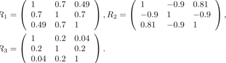
R1= 1 0.7 0.49 0.7 1 0.7 0.49 0.7 1 , R2= 1 −0.9 0.81 −0.9 1 −0.9 0.81 −0.9 1 , R3= 1 0.2 0.04 0.2 1 0.2 0.04 0.2 1 .
We took a sample of size 150 and ran the chain described in Section 3.2 for 50,000 iterations. We use the last 25,000 samples, thinned to every 50th value, to provide the output–totally 500 values. Figure 3 illustrates the plots of the simulated data and the predicted data from this mixture model.
The predictives are a good representation of the sampling density.
4.2.2 Bike time example
This real data set is about the number of bicycles traveling down the Main Yarra South Bank bike path in Melbourne, analyzed by Smith and Khaled (2012). There are 565 observations corresponding to the count of bicycles that
have passed within each hour on the working days between 12 December 2005 and 19th June 2008, excluding weekends and special days. The first column is for the period 05:01–06:00, then hourly until the period 20:01–21:00. Smith and Khaled (2012) presented a dependence structure in the bivariate case with a parametric copula.
Triple peak times, 07:01–08:00, 09:01–10:00 and 16:01–17:00, are used here to illustrate our mixture model, can be extended to higher dimensional cases in a straightforward manner. The real data are transformed according to the strategy outlined in Section 1. We ran the MCMC as in Section 4.2.1.
Figure 4 shows the scatter plots of the real data and the predictions which are in good agreement. The histogram of the number of the components in the mixture model is seen in Figure 5. The samples are computed by determining the number of distinctdi at each iteration.
5
Asymptotics
Here we present an asymptotic study of the Bayesian nonparametric model using the transformed data. We work here in the bivariate case but the results extend quite straightforwardly to higher dimensions. In this case the model can be written in the form
cP(u, v) =
Z
cρ(u, v)P(dρ),
whereP is a random Dirichlet process and in the bivariate case the correlation matrix is represented by a ρ ∈ (−1,+1). The prior for P will be chosen so that every random P will have support on [−1 +δ,1−δ] for some fixed and small δ > 0, and this is done so that cρ(u, v) is bounded away from 0 for all
ρ∈ [−1 +δ,1−δ], and likewise cP(u, v) is also bounded away from 0 for all
P. Assume c0(u, v) is the true copula density function. Then the aim is to investigate under what conditions, for all >0,
Π (c:dH(c0, c)> |(x1, y1), . . . ,(xn, yn))→0 a.s.,
wheredH(c0, c) denotes the Hellinger distance between copula density functions c0 andc. Also, here (xi, yi), are independent and identically distributed from
the density
f0(x, y) =f01(x)f02(y)c0 F01(x), F02(y)
andf01,f02are the marginal density functions ofX,Y, respectively. Note that if (x, y)∼f0 and (u, v) = (F01(x), F02(y)) then (u, v)∼c0.
To this end, define, for all >0,
A={c:dH(c0, c)> }
so that interest focuses on
Πn(A) = Π (A|(x1, y1), . . . ,(xn, yn)) = R ARn(c) Π(dc) R Rn(c) Π(dc) ,
where Rn(c) = n Y i=1 c(uni, vni) c0(ui, vi)
anduni=Fn1(xi),vni=Fn2(yi),ui =F01(xi),vi=F02(yi). The Fn1and Fn2
aren/(n+1) times the empirical distribution functions ofXandY, respectively. As is standard in Bayesian nonparametric models and the study of consis-tency (see Schwarz, 1965), we assume thatc0is in the Kullback–Leibler support of the prior, i.e.
Π (c:dK(c0, c)< η)>0
for allη >0, wheredKdenotes the Kullback–Leibler divergence; that isdk(c0, c) = R
c0log(c0/c). We will not determine the class ofc0 which lies in this support
but nevertheless it is anticipated to be large, full in fact, save for the necessity to work with correlation terms bounded away from−1 and +1.
The bounding away from−1 and +1 for the correlations are to partly ensure that, uniformly for allc,
e−nγ1 < n Y i=1 c(uni, vni) c(ui, vi) < enγ2 a.s.
for all largenand for anyγ1, γ2>0. Sufficiency for this is that the class ofcis uniformly equicontinuous and uniformly bounded away from 0. The final detail being the Clivenko–Cantelli theorem which states that
max
i∈{1,...,n}{|uni−ui|,|vni−vi|} →0 a.s.
Putting this together, we have that
1−c(u1, v1) c(u0, v0) = 1 c(u0, v0) |c(u0, v0)−c(u1, v1)|<
whenever max{|u1−u0|,|v1−v0|}< δ. Hence,
1− <c(u1, v1)
c(u0.v0) <1 +. Moreover, it is possible to show that
c(u, v) =
∞
X
j=1
wjcρj(u, v)
is uniformly equicontinuous on (0,1)2if eachρ
j∈(−1 +δ,1−δ) for someδ >0.
To see this, recall
cρ(u, v) = (1−ρ2)−1/2exp
Now let us consider the denominator of Πn(A). We can write this as In= Z n Y i=1 c(ui, vi) c0(ui, vi) n Y i=1 c(uni, vni) c(ui, vi) Π(dc).
The second product term is bounded below a.s. bye−nγ1 for all largenand for
anyγ1>0. And then, having removed this product term,
Z n Y i=1 c(ui, vi) c0(ui, vi) Π(dc)
is now a standard term and since
n−1 n X i=1 logc0(ui, vi) c(ui, vi) →dK(c0, c) a.s.
the denominator, given the assumption of c0 in the Kullback–Leibler support of Π, is bounded below by e−nη a.s. for all large n, for any η > 0. See, for
example, Barron et al. (1999) for further explanation. The numerator can be written as
Ln = Z A n Y i=1 c(ui, vi) c0(ui, vi) n Y i=1 c(uni, vni) c(ui, vi) Π(dc)
and the second product term can be bounded above a.s. byenγ2 for all largen,
for anyγ2>0. Removing this term leaves the standard term
Z A n Y i=1 c(ui, vi) c0(ui, vi) Π(dc).
This is bounded above bye−nψfor someψ >0, which depends on, provided the
prior forP satisfies condition (a) in Theorem 1 of Lijoi et al. (2005). But since we are working withP on bounded support condition (a) is trivially satisfied. There is no need for condition (b) of this theorem since thecρ(u, v) is bounded.
Hence, provided we restrict the correlations to lie in an interval bounded away from−1 and +1, we can put all the results together to establish that
Πn(A)→0 a.s.
for all >0.
References
[1] F. Autin, E. Le Pennec, and K. Tribouley. Thresholding methods to esti-mate copula density. J. Multivariate Analysis, 101:200–222, 2010.
[2] A. Barron, M. J. Schervish, and L. Wasserman. The consistency of posterior distributions in nonparametric problems. Annals of Statistics, 27:536–561, 1999.
[3] T. S. Ferguson. A bayesian analysis of some nonparametric problems.Ann. Statist., 1:209–230, 1973.
[4] C. Genest and A. C. Favre. Everything you always wanted to know about copula modeling but were afraid to ask. Journal of Hydrologic Engineering, 12:347–368, 2007.
[5] C. Genest, K. Ghoudi, and L. P. Rivest. A semiparametric estimation pro-cedure of dependence parameters in multivariate families of distributions.
Biometrika, 82:543–552, 1995.
[6] C. Genest, B. R´emillard, and D. Beaudoin. Goodness–of–fit tests for copu-las: A review and a power study. Insurance: Mathematics and Economics, 44(2):199–213, 2009.
[7] H. Ishwaran and L. F. James. Gibbs sampling methods for stick-breaking priors. Journal of the American Statistical Association, 96(453):161–173, 2001.
[8] H. Joe. Asymptotic efficiency of the two–stage estimation method for copula–based models. Journal of Multivariate Analysis, 94(2):401–419, 2005.
[9] M. Kalli, J. E. Griffin, and S. G. Walker. Slice sampling mixture models.
Statistics and Computing, 21(1):93–105, 2011.
[10] S. Kirshner. Learning with tree–averaged densities and distributions. In
NIPS, 2007.
[11] A. Lijoi, I. Pr¨unster, and S. G. Walker. On consistency of nonparametric normal mixtures for bayesian density estimation. Journal of the American Statistical Association, 100:1292–1296, 2005.
[12] X. F. Liu. Parameter expansion for sampling a correlation matrix: an efficient GPX–RPMH algorithm. Journal of Statistical Computation and Simulation, 78(11):1065–1076, 2008.
[13] A. Min and C. Czado. Bayesian inference for multivariate copulas using pair–copula constructions. Journal of Financial Econometrics, 8(4):511– 546, 2010.
[14] R. Nelsen. An introduction to copulas. Springer, New York, 2006.
[15] M. Pitt, D. Chan, and R. J. Kohn. Efficient Bayesian inference for Gaussian copula regression models. Biometrika, 93(3):537–554, 2006.
[16] L. Schwartz. On Bayes procedures. Probability Theory and Related Fields, 4:10–26, 1965.
[17] R. Silva and R. B. Gramacy. MCMC methods for Bayesian mixtures of copulas. Journal of Machine Learning Research Proceedings Track, 5:512– 519, 2009.
[18] A. Sklar. Fonctions de r´epartition `andimensions et leurs marges. Publica-tions de l’Institut de statistique de l’Universit´e de Paris, 8:229–231, 1959. [19] M. Smith and M. Khaled. Estimation of copula models with discrete
mar-gins via Bayesian data augmentation. Journal of the American Statistical Association, 107:290–303, 2012.
[20] A. Tewari, M. J. Giering, and A. Raghunathan. Parametric characteriza-tion of multimodal distribucharacteriza-tions with non–gaussian modes. Data Mining Workshops, International Conference, 0:286–292, 2011.
[21] L. Dalla Valle. Bayesian copulae distributions, with application to opera-tional risk management. Methodology and Computing in Applied Probabil-ity, 11:95–115, 2009.
[22] F. Wong, C. K. Carter, and R. Kohn. Efficient estimation of covariance selection models. Biometrika, 90(4):809–830, 2003.
[23] J. Wu, X. Wang, and S. G. Walker. Bayesian nonparametric estimation of copulas. Journal of Statistical Computation and Simulation, submitted for publication.
Figure 2: Plots of data generated from single Gaussian copula model. (a) the simulated data; (b) the predictive data.
Figure 3: Top: traces of every component (a)ρ12,(b)ρ13,(c)ρ23of the correlation matrices; bottom: histograms of every component.
Figure 4: Plots of data generated from the three mixture Gaussian copula model. (a) the simulated data; (b) the predictive data.
Figure 7: Histogram of the number of the components in the mixture Gaussian copula model for the bike time data.