Energy-Efficient Application-Aware Online Provisioning for Virtualized Clouds and
Data Centers
I. Rodero, J. Jaramillo, A. Quiroz, M. Parashar NSF Center for Autonomic Computing Rutgers, The State University of New Jersey
Piscataway, NJ, USA
{irodero,jjaram,aquirozh,parashar}@cac.rutgers.edu
F. Guim Intel Corporation
Technical University of Catalonia Barcelona, Spain
S. Poole
Computer Science and Mathematics & NCCS Divisions
Oak Ridge National Labs, TN, USA [email protected]
Abstract—As energy efficiency and associated costs become
key concerns, consolidated and virtualized data centers and clouds are attractive computing platforms for data- and compute- intensive applications. These platforms provide an abstraction of nearly-unlimited computing resources through the elastic use of pools of consolidated resources, and pro-vide opportunities for higher utilization and energy savings. Recently, these platforms are also being considered for more traditional high-performance computing (HPC) applications that have typically targeted Grids and similar conventional HPC platforms. However, maximizing energy efficiency, cost-effectiveness, and utilization for these applications while ensur-ing performance and other Quality of Service (QoS) guaran-tees, requires leveraging important and extremely challenging tradeoffs. These include, for example, the tradeoff between the need to efficiently create and provision Virtual Machines (VMs) on data center resources and the need to accommodate the heterogeneous resource demands and runtimes of these applications. In this paper we present an energy-aware online provisioning approach for HPC applications on consolidated and virtualized computing platforms. Energy efficiency is achieved using a workload-aware, just-right dynamic provi-sioning mechanism and the ability to power down subsystems of a host system that are not required by the VMs mapped to it. We evaluate the presented approach using real HPC workload traces from widely distributed production systems. The results presented demonstrated that compared to typical reactive or predefined provisioning, our approach achieves significant improvements in energy efficiency with an acceptable QoS penalty.
Keywords-Autonomic Computing; Cloud Computing; Energy
Efficiency; Virtualization; Data Center; Resource Provisioning I. INTRODUCTION
The growing scale of enterprise computing environments and consolidated virtualized data centers has made issues related to power consumption, air conditioning, and cooling infrastructures critical concerns in terms of operating costs. Furthermore, power and cooling rates are increasing eight-fold every year [1], and are becoming a dominant part of IT budgets. Addressing these issues is thus an important and immediate task for enterprise data centers.
Virtualized data centers and clouds provide the abstraction of nearly-unlimited computing resources through the elastic
use of consolidated resources pools, and provide opportu-nities for higher utilization and energy savings. These plat-forms are also being increasingly considered for traditional high-performance computing (HPC) applications that have typically targeted Grids and conventional HPC platforms. However, maximizing energy efficiency, cost-effectiveness, and utilization for these applications while ensuring per-formance and other Quality of Service (QoS) guarantees, requires leveraging important and extremely challenging tradeoffs. These include, for example, the tradeoff between the need to efficiently create and provision Virtual Machines (VMs) on data center resources and the need to accommo-date the heterogeneous resource demands and runtimes of these applications.
Existing research has address many aspects of this prob-lem including, for example, energy efficiency in cloud data centers [2][3], efficient and on-demand resource provision-ing in response to dynamic workload changes [4], and platform heterogeneity aware mapping of workloads [5]. Research efforts have also studied power and performance tradeoffs in virtualized [6] and non-virtualized environments [7] considering techniques such as Dynamic Voltage Scaling (DVS) [8]. Moreover, the thermal implications of power management have also been investigated [9]. However, these existing approach deal with VM provisioning and the config-uration of resources as separate concerns, which can result in inefficient resource configurations, and resource under-utilization, which in turn results in energy inefficiencies. The approach presented in this paper attempts to address these issues in an integrated manner by combining workload-aware provisioning with energy workload-aware allocation of VMs to resources and configuration of physical resources. Our approach builds on an technique online workload analysis and clustering.
In our previous work [10], we investigated decentralized online clustering (DOC) and autonomic mechanisms for VM provisioning to improve resource utilization [11]. This work was focused on reducing over-provisioning by effi-ciently characterizing dynamic, rather than generic, classes of resource requirements that can be used for proactive
VM provisioning. In this paper we extend this concept with an energy-aware online provisioning approach for a consolidated and virtualized computing platform for HPC applications. Specifically, we explore workload-aware, just-right dynamic and proactive provisioning from an energy perspective. Specifically, we use decentralized online clus-tering to dynamically characterize and cluster the incoming job requests across the platform in terms of their system requirements and runtimes. Our approach deals with vir-tualized cloud infrastructures with multiple geographically distributed entry points to which different users submit applications with heterogeneous resource requirements and runtimes. This results in demand for different types of VMs with heterogeneous resource configurations. Clustering allows us to identify applications tasks that require similar VM configurations. We then use these clusters for just-right VM provisioning and resource configuration so that clustered jobs with similar requirements are mapped the same host system allowing it to be configured (and unused subsystems and components to be powered down) to max-imize energy efficiency. This is based on the observation that current servers are increasing allowing specific hardware configurations that can save energy, such as turning off or downgrading specific subsystems that are not necessary to run certain applications. We also investigate how a realistic, model-driven proactive provisioning can positively impact the utilization, energy efficiency, and performance of cloud data centers. Furthermore, we not only provision available resources proactively according to expected resource re-quests, but we also actively and dynamically reconfigure the physical servers if there are no resources available with the required configurations. The overall objective of our autonomic approach is to reduce the energy consumption in the data center, while ensuring QoS guarantees. This improvement in efficiency can help service providers in-crease their profitability by reducing operational costs and environmental impact, without significant reduction in the service level delivered.
To evaluate the performance and energy efficiency of the proposed approach we use real HPC workload traces from widely distributed production systems and simulation tools. As not all of the required information is obtainable from these traces, some data manipulation (see section IV-C) was needed. We present the results from experiments conducted with three different provisioning strategies, dif-ferent workload types and system models. Furthermore, we analyze tradeoffs of different VM configurations and their impact on performance and energy efficiency. Compared to typical reactive or pre-defined provisioning, our approach achieves significant improvements in energy efficiency with an acceptable penalty in the QoS.
The overall contribution of this work is an integrated approach that combines online workload-aware provisioning and energy-aware resource configuration for virtualized
en-vironments such as clouds. The specific contributions of this paper are the following: (1) the extension and application of decentralized online clustering mechanism for energy-aware VM and resource provisioning, to bridge the gap between the two, (2) the analysis of realistic virtualization models for clouds and data centers, and (3) the analysis of performance and energy efficiency tradeoffs in cases of HPC and hybrid workloads, aimed at stating (a) the difference with typical reactive or predefined provisioning approaches and (b) the importance of just-right VM provisioning and resource configuration.
The rest of this paper is organized as follows. Sections II and III describe the clustering-based provisioning that we extend in this paper, and our energy-aware online pro-visioning approach, respectively. Section IV describes the evaluation methodology that we have followed in our exper-iments. Section V presents and discusses the experimental results. Section VI presents the related work, and section VII concludes the paper and outlines future research directions.
II. CLUSTERING-BASEDPROVISIONING
In our previous work [10], we investigated decentralized online clustering. We also presented autonomic mechanisms for VM provisioning to improve resource utilization [11]. This approach focused on reducing the over-provisioning that occurs because of the difference between the virtual resources allocated to VM instances and those contained in individual job requests. In particular, we used DOC to efficiently characterize dynamic, rather than generic (such as Amazon’s EC2 VM types [12]), classes of resource re-quirements that can be used for proactive VM provisioning. To address the inaccuracies in client resource requests that lead to over-provisioning, we explored the use of workload modeling techniques and their application to the highly varied workloads of cloud environments.
In the VM provisioning mechanism that we proposed, as with most predictive approaches, the flow of arriving jobs was divided into time periods that we call analysis windows. During each window, an instance of the clustering algorithm was run with the jobs that arrived during that window, producing a number of clusters or VM classes. At the same time, each job was assigned to an available VM as it arrived if one was provisioned with sufficient resources to meet its requirements. The provisioning was done based on the most recent analysis results from the previous analysis window. For the first window, the best option was to reactively create VMs for incoming jobs. However, the job descriptions were sent to the processing node network and by the end of the analysis window each node could quickly determine if a cluster existed in its particular region. If so, the node could locally trigger the creation of new VMs for the jobs in the next analysis window with similar resource requirements. According to [13], the time required to create batches of VM in a cloud infrastructure does not differ significantly
from the time for creating a single VM instance. Thus, the VMs for each class could be provisioned within the given time window. In order to match jobs to provisioned VMs, the cluster description could be distributed in the node network using the range given by the space occupied by the cluster in the information space. Thus, when a new job arrived, it would be routed to a node that holds descriptors for VMs that had close resource requirements.
III. ENERGY-AWAREPROVISIONING
In a cloud environment, executing application requests on the underlying resources consists of two key steps: creating VM instances to host each application request, matching the specific characteristics and requirements of the request (VM provisioning); and mapping and scheduling these requests onto distributed physical resources (resource provisioning). In this work, we extend the concept of clustering-based VM provisioning described previously in two ways. On the one hand, we add energy awareness to the clustering-based VM provisioning, from the perspective of the energy associated to over-provisioning and re-provisioning costs. On the other hand, we implement a workload-aware resource provisioning strategy based on energy-aware configurations of physical servers, and optimizing the mapping of VMs to those servers using workload characterization. Our approach is implemented in different steps; each step has different functions, but all have common objectives. The input of our approach is a stream of job requests in the form of a trace with job arrival times and their requirements. As described in the previous section, we divide the trace into analysis windows. Since we focus on a realistic approach, our policy is characterized by having analysis windows of a fixed duration with variable job arrival times, rather than by having a fixed number of jobs in each window. We consider an analysis window with duration of one minute, in order to provide a more realistic distribution for job queuing times. Moreover, in order to model the system with multiple entry points for user requests, we have used traces with a high rate of requests (see section IV-C). The different steps of our strategy are briefly described below:
• Online clustering. For each analysis window, it
clus-ters the job requests of the input stream based on their requirements. It returns a set of clusters (groups of job requests with similar requirements) and a set of outliers (job requests that do not match any of the clusters found).
• VM provisioning. Using the groups of jobs we
provi-sion each job request with a specific VM configuration. To do this, we define a greater number of classes of VMs, each described very finely, rather than a smaller number of coarsely described classes. It also tries to reuse existing VM configurations in order to reduce the re-provisioning costs.
• Resource provisioning. We group VMs with similar
configurations together and allocate resources for them that are as closely matched as possible to their require-ments. To do this, we provision resources using work-load modeling based on profiling (see section IV-D), taking into account specific hardware configurations available from the underlying servers. Specifically, we apply specific hardware configurations that can save energy (such as low power modes) for those subsystems that are not required.
Our approach attempts to optimize energy efficiency in the following ways:
• Reducing the energy consumption of the physical
re-sources by powering down subsystems when they are not needed.
• Reducing over-provisioning cost (waste of resources)
through efficient, just-right VM provisioning.
• Reducing re-provisioning cost (overhead of VM
in-stantiation) through efficient proactive provisioning and VM grouping.
In the following subsections we describe the previously discussed steps in detail.
A. Clustering Strategy
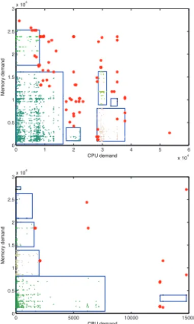
As described previously, our approach starts with the clustering algorithm, using the requirements from the input stream of job requests, and returning groups of jobs that have similar requirements. To group the incoming requests in different VMs we use a clustering algorithm as proposed in [11]. The algorithm takes the incoming requests in a given analysis window and creates clusters from groups of requests with similar requirements. When a request does not belong to any of the clusters found, it is said to be an outlier. The clustering algorithm can be done with as many dimensions as wanted, but as the number of dimensions grows, so does the complexity of the space, and results are harder to analyze. The dimensions we take into account in this analysis include the requested execution time (T), requested number of processors (N), requested amount of memory and storage, and network demand. To reduce the search space, we perform the analysis in two steps. The first step runs the clustering algorithm with only two dimensions: the required memory versus a derived value of execution time and number of processors that represents CPU demand (C in equation 1). The value of 100 in Equation 1 is a normalization factor that represents the duration in seconds of a reference job.
C=N×T
100 (1)
Figure 1 shows two plots of the clustering results ob-tained from two different analysis windows. Each rectangle represents a cluster and contains a set of points inside representing job requests that may be grouped together, with
stars representing outliers. Both plots have six clusters but there are important differences between them. Consequently, the VM classes associated to the different clusters will be different in the two different analysis windows.
0 1 2 3 4 5 6 x 10⁴ 0 0.5 1 1.5 2 2.5 3x 10 4 CPU demand Memory demand 0 5000 10000 15000 0 0.5 1 1.5 2 2.5 3x 10 4 CPU demand Memory demand
Figure 1: Clusters of two different analysis windows
In the second step, the clustering is run on requested storage and network demand over the job requests of each cluster obtained in the first step. With the resulting clusters, we are able to allocate jobs to specific VM types. Using the workload characterization model described in section IV-D, we can also allocate job requests matching similar resource requirements together on the appropriate physical servers. Also, using these clusters and the workload characterization, we are able to proactively configure the subsystems of the physical resources appropriately.
B. VM Provisioning
As previously discussed, we provision VM classes using the clusters obtained with DOC. For these clusters, we provision finely described classes of VMs rather than generic ones, as it is usually done (e.g. Amazon’s EC2 [12]). The strategy consists on grouping the requests of a given cluster together in the same class of VM, proactively provisioning one class of VM for each cluster. Requests considered as outliers are handled independently.
The main objective is to reduce over-provisioning cost (due to under-utilization) and re-provisioning cost (the delay of configuring and loading a new VM instance). More details regarding the metrics are shown in section IV-E.
VM provisioning is done based on the most recent clustering results from the previous analysis window, and thus it is possible to overlap the clustering computa-tion with the creacomputa-tion of VM batches. Specifically, VM
provisioning is performed as follows: given a set of analysis windows (w1, ..., wn), the job requests
belong-ing to each analysis window (reqw1, ..., reqwn), sets of
clusters {(cw11, ..., cw1m), ...,(cwn1, ..., cwnp)} and outliers
(ow1, ..., own) corresponding to each analysis window
(ob-tained by applying the clustering algorithm described in the previous subsection), assigning a specific VM class to each job request. A specific VM class can be assigned to each job request by identifying the configuration characteristics (e.g. amount of memory) of the cluster to which the job belongs. If the job was found to be an outlier, a new VM class can be reactively provisioned for it. Outliers therefore incur extra overhead, but by definition are expected to be the exception rather than the norm. Algorithm 1 finds the appropriate VM class for a given job request (req) based on the input described above, and the status of the system (existing VM classes, i.e. V in Algorithm 1). The complete VM provisioning process iterates over all job requests of each analysis window as is shown in Equation 2.
∀i: 1≤i≤n:∀req∈reqwi:vm prov(req) (2)
For the first analysis window, the algorithm reactively creates VMs classes for all incoming job requests. In case of an outlier, the algorithm provisions it with a new VM class configured with the requirements of the job request. In case of a job request that matches a cluster, the algo-rithm provisions it with a VM class configured with the requirements of that cluster. It means that the provisioned VM class is configured with the highest requirements of the cluster in order to be able to accommodate all requests of that cluster in that VM. Although the above procedure does result in some over-provisioning, it reduces the overhead for re-provisioning with new VM classes. The helper conf ig
function returns the VM configuration that matches the requirements of a specific job request or cluster. Once a job request has been provisioned with a VM class, that VM class becomes available in the system.
For subsequent analysis windows, if the job request matches a cluster, the algorithm provisions it with an in-stance of an existing VM class configured for that cluster. Otherwise, the algorithm tries to correlate the job request with other existing VM classes to find the closest match
(correlatefunction). This reduces the re-provisioning cost
because the job request can usually be provisioned with an existing VM instance, therefore saving the VM instantiation delay. To correlate a given job request with the previously defined VM classes, we use the corners of the clusters’ bounding boxes (i.e. the area or space occupied by the clusters) in the two-dimensional space described in the previous subsection. If the requirements of a job are com-pletely covered by the top right corner of an existing cluster, then it can be provisioned with the corresponding VM class, because the resource configuration is enough to meet
Algorithm 1VM Provisioning per Job Request (vm prov)
Input:
(w1, . . . , wn): analysis windows req: job request{req∈reqwi}
{(cw11, . . . , cw1|cw1|), . . . ,(cwn1, . . . , cwn|cwn|)}: clusters
(ow1, . . . , own): outliers V: current set of VM classes
Output:
Updated set of VM classes
V←V
ifreq∈reqw1 then
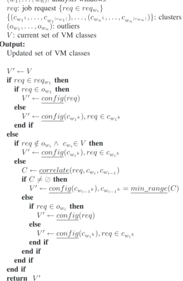
ifreq∈ow1 then V←conf ig(req) else V←conf ig(c w1k), req ∈cw 1k end if else ifreq /∈owi∧ cwi∈V then V←conf ig(c wik), req ∈cwik else C←correlate(req, cwi, cwi−1) ifC=then V←conf ig(c wi−1k), cwi−1k =min range(C) else ifreq∈owi then V←conf ig(req) else V←conf ig(c wik), req∈cwik end if end if end if end if return V
the job’s requirements. However, as discussed previously, some level of over-provisioning may occur. Algorithm 2 implements thecorrelatefunction. Given a job request and the clusters of the current and previous analysis windows, it returns a set of clusters of the previous analysis window that are correlated with the job request. Specifically, if the job request matches a cluster in the current analysis window, the algorithm selects all clusters from the previous analysis window that include that cluster. In Algorithm 2, ci.topX
and ci.topY are the values of the X and Y axes of the top
corner of cluster ci, respectively. If the job request is an
outlier in the current analysis window, the algorithm selects all clusters from the previous analysis window that contain the point that represents the job request. In Algorithm 2,
req.X and req.Y are the values of the X and Y axes of
the point that represent the job request in a two-dimensional clustering space, respectively.
Algorithm 2 correlatefunction
Input:
req: job request
{cwi1, . . . , cwi|cwi|}: clusters of current window
{cwi−11, . . . , cwi−1
|cwi
−1
|}: clusters of previous window
Output: Set of clusters C← forj = 1, . . . ,|cwi−1|do if ∃k:req∈cwik then if cwik.topX≤cwi−1 j .topX ∧ cwik.topY≤cwi−1 j .topY then C←cwi−1j end if else if req.X≤cwi−1 j .topX∧req.Y≤cwi−1 j .topY then C←cwi−1j end if end if end for return C
Figure 2 illustrates a simple scenario with clusters from two different analysis windows. It shows two clusters in each analysis window. Requests in the common area between
cluster1ofwini−1andcluster2ofwinican be mapped to
the VM class that satisfiescluster1 ofwini−1. Since some
job requests withincluster1ofwini are not within the area
of cluster1 ofwini−1, not all job requests of cluster1 of wini can be satisfied by the VM configuration ofcluster1
of wini−1. However, all requests of both clusters of wini
can be mapped to the VM class that satisfies cluster2 of
wini−1.
Figure 2: Example of correlation between clusters of two different analysis windows
If the job request matches one or more clusters of the previous analysis window, the algorithm selects the VM class of lowest resource configuration. To do this, it uses
the min range function. Equation 3 defines min range
function, whereC is a set of clusters andrange(c)returns the range (i.e. the area in a two-dimensional space) of cluster
c.
min range(C) =cmin⇔ ∀ci∈C: (3)
range(cmin)≤range(ci)
If the job request does not match any cluster from the previous analysis window but matches a cluster in the current analysis window the algorithm provisions it with a VM class configured with the requirements of that cluster. If the job request is an outlier in the current analysis window,it provisions the job request with a VM class meeting the job request requirements.
C. Resource Provisioning
Once a job request has been provisioned with a specific VM class, it is provisioned with a specific VM instance. Since we proactively create VM batches, we try to reuse existing VM instances from the previous analysis window rather than creating new ones. Furthermore, we allocate physical servers to the VMs that are as closely matched as possible to their requirements. In contrast to other typical approaches that allocate job requests with non-conflicting, i.e. dissimilar, resource requirements together on the same physical server, our policy is to allocate job requests with similar resource requirements together on the same physical server. This allows us to downgrade the subsystems of the server that are not required to run the requested jobs in order to save energy. To do this, we consider specific configurations of the physical servers’ subsystems to reduce their energy demand. Specifically it follows an energy model that leverages previous research on energy-efficient hardware configurations (e.g. low power modes) in four different dimensions:
• CPU speed using Dynamic Voltage Scaling (DVS).
We are able to reduce the energy consumed by those applications that are, for example, memory-bound [14].
• Memory usage. For those applications that do not
require high memory bandwidth we consider the pos-sibility of slightly reducing the memory frequency or possibly shutting down some banks of memory in order to save power [15].
• High performance storage. It may be possible to power
down unneeded disks (e.g. using flash memory devices that require less power) or by spinning-down disks [16].
• High performance network interfaces. It may be
pos-sible to power down some network subsystems (e.g. Myrinet interfaces) or using idle/sleep modes.
We have implemented two different resource provisioning strategies: a static approach where physical servers maintain their initial subsystem configuration, and a dynamic one that allows the physical servers to be reconfigured dynamically.
Algorithm 3 Static Resource Provisioning
Input:
req: job request
V Mclass: VM class ofreq job request
(reqcpu, reqmem, reqdisk, reqnic): resource requirements S = (s1, . . . , sn): physical servers
{(s1vm1, . . . , s1vmp), . . . ,(snvm1, . . . , snvmq)}: VMs
Output:
VM instance (on a specific physical server)
S=match reqs(req, S)
if S=then
return {req cannot be provisioned at this time}
else Svm=match vm(V M class, S) if Svm=then sk =less reqs(S) sk ←vm=new vm(V Mclass) return vm else vm =vm less reqs(Svm) return vm end if end if
The algorithm followed by the static resource provisioning approach for a given job is shown in Algorithm 3. For readability and space limitations, we have simplified the algorithm assuming that each job request is provisioned with a single VM instance. The complete approach returns a set of VMs that are then mapped to a set of physical servers. Given the VM class associated to the job request
(V Mclassin Algorithm 3) and the resource requirements of
a job request(reqcpu, reqmem, reqdisk, reqnic), the available
physical servers(s1, . . . , sn), and the existing VMs in each
server {(s1vm1, . . . , s1vmp), . . . ,(snvm1, . . . , snvmq)}, it
re-turns the most appropriate VM instance to run the requested job. The resource requirements of the job request are the CPU, memory, storage and network demand, respectively.
First, the algorithm discards the physical servers that do not match the resource requirements of the job request. To do this, it uses the match reqs function, which is defined in Equation 4.
match reqs(req, S) =S⇔S⊆S ∧ ∀s
i∈S: (4)
(sicpu ≥reqcpu∧simem ≥reqmem ∧ sidisk ≥reqdisk∧sinic ≥reqnic )
If a physical server that matches the job request requirements is not available, the job request cannot be provisioned with a VM instance; thus, the algorithm does not return any VM instance at that time. In this case, if we follow a First Come First Serve (FCFS) scheduling policy with the
static approach, a request may remain queued (thus blocking all following queued jobs) until a server with the required configuration becomes available. If there is available a physical server meeting the job request requirements, the algorithm selects a server that can host VM instances with sufficient configured resources to run the job request. To do this, the algorithm discards the servers that do not match the requirements of the job request’s VM class using the
match vm function. This function is defined in Equation
5, where c is the VM class of the job request, S is a set of servers, ccpu, cmem, cdisk, cnic are the required CPU,
memory, disk and network by the job request’s VM class, respectively, and vmcpu, vmmem, vmdisk, vmnic are the
CPU, memory, disk and network configuration of the VM instancevm, respectively.
match vm(c, S) =Svm⇔Svm⊆S ∧ ∀s∈Svm:
(5) (∃vm∈s:vmcpu≥ccpu∧vmmem≥cmem ∧
vmdisk ≥cdisk∧vmnic≥cnic )
If a server that matches the requirements of the job re-quest’s VM class is not available, we create a new VM instance reactively (new vm function in Algorithm 3) on the physical server with lowest power requirements (i.e. with the most subsystems disabled or in low power mode) and hosting the fewest job requests, and we provision the job request with the new vm instance (vm in Algorithm
3). To select the server that best matches the conditions described above, the less reqs function is used. Given a set of servers, this function returns the most appropriate one. If there are various servers hosting available VMs that match the job request’s VM class, we first employ the VMs allocated in servers hosting the fewest job requests, lowest power requirements, and with the lowest resource configuration (e.g. memory configured). To do this, the
vm less reqs function, which is similar toless reqs but
returning a VM instance rather than a server, is used. Due to space limitations, we do not present a formal description
ofvm less reqsandless reqsfunctions. Also, we do not
show the algorithm that implements the dynamic resource provisioning approach. However, we summarize the main differences with respect to the static approach below.
In our dynamic approach, when required physical re-sources are unavailable, we reconfigure an available physical server to provide the appropriate characteristics and then provision it. Specifically, we can reconfigure servers if they are idle, but if there are no idle servers available, we can reconfigure only those servers that are configured to use fewer subsystems than those that are requested (if a server is configured to deliver high memory bandwidth, we cannot re-configure it to reduce its memory frequency, since that would negatively impact jobs already running on it. However, if a server is configured with reduced memory frequency, we can reconfigure it to deliver full memory bandwidth without
negatively impacting running jobs). Moreover, since we still do not consider VM migration, we try to fill servers with requests of similar types. Not only does this efficiently load servers, it allows more servers to remain fully idle, which allows them to be configured to host new job requests.
IV. EVALUATIONMETHODOLOGY
To evaluate the performance and energy efficiency of the proposed approach, we use real HPC workload traces from widely distributed production systems. Since not all of the required information is obtainable from these traces, some data manipulation was needed, such as the trace pre-processing described in section IV-C. In order to separate concerns and because the batch simulation of clustering over all analysis windows is a time-consuming task, we perform the experiments in two steps. First, we compute the clusters for each analysis window (driven by the job arrival times) using the distributed clustering procedure over the input trace. Afterwards, the original trace is provided as input to the simulator, along with the configuration files and an additional trace file that contains requirements and the output of the clustering for each job request (analysis window, cluster number, corners of the cluster, etc.). We obtain the results from the simulator output and process the output traces post-mortem.
A. Simulation Framework
For our experiments, we have used the kento-perf simula-tor (formerly called Alvio [17]), which is a C++ event driven simulator that was designed to study scheduling policies in different scenarios, from HPC clusters to multi-grid systems. In order to simulate virtualized cloud data centers we have extended the framework with a virtualization (VM) model. Due space limitations, in this paper we only describe the main characteristics of this model. Our VM model considers that different VMs can run simultaneously on a node if it has enough resources to create the VM instances. Specifically, a node must have an available CPU for each VM instance and enough memory and disk for all VMs running on it. This means that the model does not allow sharing a CPU between different VMs at the same time. Although this limitation in the model may penalize our results, some simplification was needed to reduce the model’s complexity. Moreover, as we have not modeled VMs with multiple CPUs yet, we configure N VMs with a single CPU each in order to provision a VM for an application request that requires N CPUs. However, we have considered requests with high demand for memory in order to experience memory conflicts between different VMs within the physical nodes. Therefore, the model simulates the possible conflicts and restrictions that may occur between VMs with multiple CPUs. We have modeled the overhead of creating VM instances with a fixed time interval of one minute, which is the duration of the
analysis windows. It allows us to overlap the clustering com-putation with the creation of VM instances. We have also modeled four pre-defined classes of VMs for the reference reactive approach (using 0.5, 1, 2 and 4 GB of memory). We have simulated a homogeneous cluster system based on servers with 4 CPUs and 8GB of RAM each.
B. System Power Model
Our server power model is based on empirical data, the technical specifications from hardware vendors, and existing research. The actual power measurements were performed using a “Watts Up? .NET” power meter. The meter was attached between the wall power and an Intel Xeon-based server with a quad-core processor, 8 GB of RAM, two disks, and both Gigabit Ethernet and Myrinet network interfaces. Using our measurements and existing research [18][19] (e.g. to obtain the power required by a subsystem scaling from the total server power), we configured the simulations with the power required for the different subsystems and the switch latencies shown in Table I. The model has some simplifications, such as using a coarse grain level for switch latencies (we use longer latencies) and using a fixed switch latency between different power modes of a subsystem. Specifically, for the CPU we consider three different states: running mode, i.e., C0 C-state and highest P-state (“Running” in Table I), low power mode, i.e., C0 C-state and the deepest P-state (“Low” in Table I), and idle state, i.e., (C-state different to C0) (“Idle” in Table I). For the memory subsystem, we consider two states (regular and low power mode). We estimate the memory energy consumption from the power models based on RDRAM memory throttling discussed in [20][21]. Although the techniques described in [20][21] are not available in our physical testbed, we consider low power modes for memory to be supported by modern systems. For the storage subsystem, we used actual power measurements and the disk characteristics such as in [22], but assuming newer technology. For the network subsystem we consider two different states: regular and idle. The idle state corresponds to the hardware sleep state in which the network interface is in listening mode.
Since we assume that modern systems use power manage-ment techniques within the operating system, we consider
Table I: Power requirements (in watts) and delay associated to different server subsystems
Subsystem Running Low Idle Latency
CPU 155 w 105 w 85 w 0.01 s Memory 70 w 30 w - 0.06 s Disk 50 w - 10 w 2 s NIC 15 w - 5 w 0.15 s Others 110 w - - -Total 400 w - -
-low power modes in our simulations when the resources are idle. As well as taking into account the power required by the previous subsystems, we also include in our model the power required by other components such as mother-board, fans, etc. Therefore, some fixed amount of power is always required, independently of the specific physical server configuration used. However, we do not consider the power required for cooling and to manage external elements. Although this model is not completely accurate with respect to applications’ execution behaviors, it gives us a base framework to evaluate the possibilities of our approach. C. Workloads
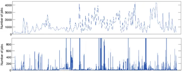
In our previous work [11], we considered a very high number of requests in each analysis window. However, we did not follow the actual request arrival times from the HPC traces used, because the arrival rates of these traces were not high enough. In order to model the heterogeneous nature of virtualized cloud infrastructures with multiple geographically distributed entry points, we required traces with different application requirements and high arrival rates. In the present work, we have used traces from the Grid Observatory [23], which collects, publishes, and analyzes data on the behavior of the EGEE Grid [24]. This trace meets our needs because it currently produces one of the most complex public grid traces and meets our need. The frequency of request arrivals is much higher in contrast to other large grids such as Grid5000. Figure 3 compares the selected trace from Grid Observatory and a Grid5000 trace from the Grid Workloads Archive [25]. Note that both X and Y axis of the figures are in different scales (i.e. X axis is by minutes for EGEE and by hours for Grid5000).
Figure 3: Request arrivals of EGEE (top) and Grid5000 (bottom) traces, in jobs/minute and job/hour, respectively
Since the traces are in different formats and include data that is not used, they are pre-processed before being input to the simulation framework. First, we convert the input traces to Standard Workload Format (SWF) [26]. We also combine the multiple files of which they are composed into a single files. Then, we clean the trace in SWF format in order to eliminate failed jobs, cancelled jobs and anoma-lies. Finally, we generate the additional requirements that are not included in the traces. For instance, traces from
Grid Observatory do not include required memory, and the mapping between gLite (i.e. the EGEE Grid middleware) and the Local Resource Management Systems (LRMS) that contains such information is not available. Thus, we included memory requirements following the distribution of a trace from Los Alamos National Lab (LANL) CM-5 log [26], and we included the disk and network demand based on a workload characterization (see following subsection) using a randomized distribution. Although the memory require-ments are obtained from a dated trace, we scaled them to the characteristics of our system model. We estimate that similar results can be obtained using a resource requirement distribution from other traces or recent models.
D. Workload Characterization Model
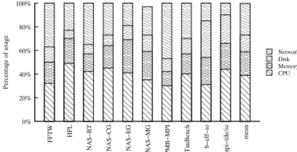
In order to perform an efficient mapping of the incoming job requests to physical servers, we need their require-ments in terms of subsystems utilization. Specifically, we consider CPU utilization, requested memory and storage, and communication network usage. As the traces found from different systems do not provide all the information needed for our analysis, we needed to complete them using a model based on benchmarking a set of applications. We profiled standard HPC benchmarks with respect to behaviors and subsystem usage on individual computing nodes rather than using a synthetic model. To do this we used different mechanisms such as commands from the OS (e.g. iostat or netstat) and PowerTOP from Intel. A comprehensive set of HPC benchmark workloads has been chosen. Each stresses a variety of subsystems - compute power, memory, disk (storage), and communication (network). The relative proportion of stress on each subsystem of each benchmark is shown in Figure 4. We do not provide more details regarding workload profiling due to the space limitations.
0% 20% 40% 60% 80% 100% mean mpi − tile/io b − eff − io TauBench PMB − MPI NAS − MG NAS − EG NAS − CG NAS − BT HPL FFTW Percentage of usage Network Disk Memory CPU
Figure 4: Percentage of CPU, memory, disk and network usage per benchmark
After calculating the average percentage of CPU, memory, storage and network usage for each benchmark, we ran-domly assign one of these ten benchmark profiles to each request in the input trace, following a uniform distribution.
E. Metrics
We evaluate the impact of our approach on the following metrics: makespan (workload execution time, which is the difference between the earliest time of submission of any of the workload tasks, and the latest time of completion of any of its tasks), energy efficiency (based on both static and dynamic energy consumption, and energy delay product), resource utilization (based on CPU utilization), average re-quest waiting time (as a QoS metric), and over-provisioning cost (to show the accuracy with which the different data analysis approaches can statically approximate the resource requirements of a job set). We define over-provisioning cost for resource R (e.g. memory) in each analysis window
i as the average difference between requested (Q) and provisioned (P) resources for the set of jobs j in that window (see Equation 6).
OR i = 1 N N j=1 PR ij −Q R ij (6) V. RESULTS
We have conducted our simulations using different vari-ants of the provisioning strategies, workloads and system models described in the previous sections. Specifically, we have evaluated the following provisioning strategies:
REACTIVE - implements the reactive or pre-defined pro-visioning implemented by typical cloud providers, such as Amazon EC2 [12]. Specifically, it provision with four classes of VMs as described in section IV-A. It follows a FCFS scheduling policy to serve requests (in the same order of arrival), and implements a First-Fit resource selection policy to provision physical servers. This means that it maps the provisioned VMs to the first available physical servers that match the requests requirements.
STATIC - implements our proposed provisioning approach based on clustering techniques with a static approach to configure the resources. It means that the servers config-urations remain constant; therefore a physical server can host only applications that match its specific characteristics. Specifically, we consider eight classes of configurations (one for each possible combination of their subsystems configuration) and we model the same amount of servers with each one.
DYNAMIC - implements our proposed provisioning ap-proach similarly to the STATIC strategy but implementing dynamic resource re-configurations when they are necessary. This means that when there are not available resources configured with the requested configuration, it re-configures servers reactively in order to service new application re-quests.
We have generated three different variants of the workload described in section IV-C in order to cover the peculiarities of three different scenarios:
HPC- follows the original distribution of the EGEE work-load described in the previous section, which is mostly composed of HPC applications with long execution times and high demand for CPUs.
SERVICE - follows an application pattern of shorter exe-cution times and fewer resource requirements (i.e. service applications characteristics), but respecting the arrival rate and distribution of the original trace.
MIXED - includes both HPC and SERVICE profiles in order to address the heterogeneous nature of clouds. We will consider this workload variant as the reference one to obtain conclusions because it covers a wider range of application request profiles.
In order to evaluate the impact of the system in our approach we also have evaluated three different setups depending of their size: SMALL (more than 1000 servers), MEDIUM (more than 2000 servers), and LARGE (more than 4000 servers). We have conducted experiments with the different workloads and systems models (all possible com-binations) to compare our proposed strategies with respect to the reference approach (REACTIVE). The experiments attempt to state that our proposed policies can save energy consumption while maintaining a similar execution and waiting times (QoS given to users). The experiments also attempt to state that the proposed strategies do not fall in underutilization of the resources while they reduce the over-provisioning cost.
Figures 5, 6, 7, 8 and 9 show the relative makespan, en-ergy consumption, Enen-ergy Delay Product (EDP), utilization and average waiting time results, respectively. In each of these figures, subfigures (a), (b) and (c) show the results obtained with each provisioning policy and workload vari-ant. For readability, the results are normalized to the results obtained with the REACTIVE approach for each workload variant. Subfigure (d) shows the results obtained with the MIXED workload normalized to the result obtained with the REACTIVE approach and MEDIUM system size. It allows us to analyze the impact of the system size on each metric. In order to show the trends of the results obtained using the different workload variants, subfigure (e) shows the results obtained with the MEDIUM system model normalized to the result with the lowest value. Although in some HPC systems waiting times may be longer, we consider average waiting time rather than average response time because in our results the execution time is the leading portion of the response time, which is probably the most appropriate metric to measure the QoS given to users.
Figures 5 and 9 show that both makespan and average waiting time results follow similar patterns. With the RE-ACTIVE strategy, the delays are shorter than those obtained with our approach, and with the STATIC strategy, they are much longer than with DYNAMIC. This is explained by the fact that using the STATIC provisioning strategy with avail-able resources, matching the request requirements is harder
because the number of resources with the same subsystem configuration is fixed. Since the scheduling strategy follows a FCFS policy to serve the incoming requests, the average waiting times are much longer with the STATIC approach and therefore the makespan also becomes longer (more than 5% on average). However, the same strategies present differ-ent results depending on the workload type and system size. On the one hand, with larger system setups the differences between the provisioning strategies are lower. This is due to larger systems providing a larger number of servers, thus facilitating provisioning for specific resources. On the other hand, with SERVICE workload the trends of the results are different than those observed with the other workloads. In particular, makespan is shorter with DYNAMIC than with REACTIVE using MEDIUM and LARGE system models while the average waiting time is much shorter with the REACTIVE approach. This is explained by the fact that although run times are much shorter in relation to other workloads, the overhead of creating new VM instances is much larger. It is especially significant with the LARGE system model because there are more available resources. Moreover, with the STATIC approach the results are worse because resource limitations cause job blocking (especially with the SMALL system model). However, the delays shown in Figure 9b are also very long with STATIC and DYNAMIC strategies because we have not considered the overheads of creating new VM instances as part of the waiting time and these overheads are critical in this scenario. We will consider SERVICE workload as a specific use case and MIXED workload as the reference one for our comparisons because as is shown in Figure 5e makespan with SERVICE workload is several times shorter than with the other ones.
Although the makespan is shorter with the REACTIVE approach, the energy efficiency obtained with our proposed strategy is better than that obtained with the REACTIVE approach. Specifically, both STATIC and DYNAMIC approaches obtain between 8-25% energy savings with respect to the REACTIVE approach (depending on the scenario). With the DYNAMIC approach, the EDP is between 2-25% lower than the REACTIVE approach (depending on the scenario). However, although the energy consumption is lower with the STATIC approach with respect to the REACTIVE approach, the EDP is higher. The specific configuration of the resource subsystems is the main source of energy savings. Our proposed strategy provides the largest energy savings with respect to the REACTIVE approach when the SERVICE workload is used. In this scenario, the overhead of creating VMs (which also consumes energy) has a strong impact on energy consumption. Furthermore, the energy efficiency is slightly worse with the DYNAMIC approach with larger system models due to higher over-provisioning costs. However, in smaller systems the energy efficiency is better with the DYNAMIC approach because the makespan is longer with
0.85 0.9 0.95 1 1.05 1.1 1.15 1.2 1.25 LARGE MEDIUM SMALL REACTIVE STATIC DYNAMIC (a) HPC workload 0.9 1 1.1 1.2 1.3 LARGE MEDIUM SMALL REACTIVE STATIC DYNAMIC (b) SERVICE workload 0.9 0.95 1 1.05 1.1 1.15 LARGE MEDIUM SMALL REACTIVE STATIC DYNAMIC (c) MIXED workload 0 0.5 1 1.5 2 2.5 LARGE MEDIUM SMALL REACTIVE STATIC DYNAMIC (d) MIXED vs MEDIUM 0 5 10 15 20 25 30 35 LARGE MEDIUM SMALL REACTIVE STATIC DYNAMIC
(e) MEDIUM system model Figure 5: Relative makespan
0.85 0.9 0.95 1 1.05 LARGE MEDIUM SMALL REACTIVE STATIC DYNAMIC (a) HPC workload 0.65 0.7 0.75 0.8 0.85 0.9 0.95 1 1.05 1.1 LARGE MEDIUM SMALL REACTIVE STATIC DYNAMIC (b) SERVICE workload 0.8 0.85 0.9 0.95 1 1.05 LARGE MEDIUM SMALL REACTIVE STATIC DYNAMIC (c) MIXED workload 0 0.5 1 1.5 2 2.5 LARGE MEDIUM SMALL REACTIVE STATIC DYNAMIC (d) MIXED vs MEDIUM 0 5 10 15 20 25 30 35 40 45 LARGE MEDIUM SMALL REACTIVE STATIC DYNAMIC
(e) MEDIUM system model Figure 6: Relative energy consumption
0.85 0.9 0.95 1 1.05 1.1 1.15 1.2 1.25 LARGE MEDIUM SMALL REACTIVE STATIC DYNAMIC (a) HPC workload 0.6 0.7 0.8 0.9 1 1.1 1.2 LARGE MEDIUM SMALL REACTIVE STATIC DYNAMIC (b) SERVICE workload 0.8 0.85 0.9 0.95 1 1.05 1.1 LARGE MEDIUM SMALL REACTIVE STATIC DYNAMIC (c) MIXED workload 0 0.5 1 1.5 2 2.5 LARGE MEDIUM SMALL REACTIVE STATIC DYNAMIC (d) MIXED vs MEDIUM 0 200 400 600 800 1000 1200 1400 LARGE MEDIUM SMALL REACTIVE STATIC DYNAMIC
(e) MEDIUM system model Figure 7: Relative Energy Delay Product (EDP)
0.75 0.8 0.85 0.9 0.95 1 1.05 1.1 LARGE MEDIUM SMALL REACTIVE STATIC DYNAMIC (a) HPC workload 0.6 0.7 0.8 0.9 1 1.1 LARGE MEDIUM SMALL REACTIVE STATIC DYNAMIC (b) SERVICE workload 0.8 0.85 0.9 0.95 1 1.05 LARGE MEDIUM SMALL REACTIVE STATIC DYNAMIC (c) MIXED workload 0.7 0.75 0.8 0.85 0.9 0.95 1 1.05 LARGE MEDIUM SMALL REACTIVE STATIC DYNAMIC (d) MIXED vs MEDIUM 0.95 1 1.05 1.1 1.15 1.2 1.25 LARGE MEDIUM SMALL REACTIVE STATIC DYNAMIC
(e) MEDIUM system model Figure 8: Relative utilization
0.9 0.95 1 1.05 1.1 1.15 1.2 1.25 1.3 LARGE MEDIUM SMALL REACTIVE STATIC DYNAMIC (a) HPC workload 0 5 10 15 20 25 LARGE MEDIUM SMALL REACTIVE STATIC DYNAMIC (b) SERVICE workload 0.99 1 1.01 1.02 1.03 1.04 1.05 LARGE MEDIUM SMALL REACTIVE STATIC DYNAMIC (c) MIXED workload 0 0.5 1 1.5 2 2.5 LARGE MEDIUM SMALL REACTIVE STATIC DYNAMIC (d) MIXED vs MEDIUM 0 5 10 15 20 25 30 LARGE MEDIUM SMALL REACTIVE STATIC DYNAMIC
(e) MEDIUM system model Figure 9: Relative average waiting time
STATIC and therefore, with STATIC, the servers consume less energy, but for a longer time. Although a larger system should consume more energy, the workload may be executed in a shorter time, and thus the predominant factor of energy efficiency is not the system model. In contrast, the type of workload has a strong impact on the energy efficiency as well as the provisioning strategy.
In contrast to the other metrics whose results are very dependent on the size of the system model, utilization is similar with different system models and workload types. This is because quantitatively the utilization of the resources is very high (between 59% and 93% with the average over 85%) due to the fact that systems are very loaded (high job arrival rate and high demand for resources such as memory). In Figure 8 we can appreciate that by using the REACTIVE approach the utilization is higher because configurations without resource restrictions (in terms of subsystems configuration) facilitates mapping VMs to phys-ical servers. In contrast, with the STATIC approach the utilization is lower because, during the periods of time that specific subsystem configurations are not available, some resources may remain idle. We estimate that the utilization could be lower if we would consider VM configurations with different numbers of CPUs. However, in the presented results, memory conflicts in the allocation of VMs limit resource utilization. Although we have presented results that focus on the resource utilization ratio, memory usage is more efficient with our provisioning approach in contrast to REACTIVE provisioning. Figure 10 shows the average over-provisioning cost of the analysis window for each provisioning strategy.
The memory over-provisioning cost difference between
0 100 200 300 400 500 600 700 800 Memory (MB) Analysis window REACTIVE STATIC 0 100 200 300 400 500 600 700 800 Memory (MB) Analysis window REACTIVE DYNAMIC
Figure 10: Average difference between requested memory for jobs and the provisioned one
REACTIVE and our approach is quite large (4.5-6.3 times lower with our approach in contract to the REACTIVE one). Specifically, the over-provisioning cost is 390 MB on average for the REACTIVE approach, and 61 MB and 86 MB on average for our STATIC and DYNAMIC approach, respectively. Furthermore, the DYNAMIC approach presents a higher level of over-provisioning, and the points in Figure 10 are less concentrated with respect to STATIC. This is due to the fact that some over-provisioning situations may occur when dynamically reconfiguring resources that are already hosting requests with less resource requirements. To improve this particular inefficiency, we suggest migrating VMs when a resource is required to be reconfigured resulting in nodes hosting requests that best fit their configurations.
0.85 0.9 0.95 1 1.05 AVG Wait Utilization Energy Makespan 4 VM classes 6 VM classes 8 VM classes 10 VM classes
Figure 11: Relative results using different number of VM classes
We have also conducted another experiment to analyze tradeoffs between different VM configurations and the im-pact on the previously analyzed metrics. On the one hand, Figure 11 presents the results obtained using the REACTIVE approach with MIXED workload and MEDIUM system model, which is an intermediate (and probably the most representative) setup. The results are given using different numbers of VM classes, but all of them are in the same range of memory configuration (up to 4GB, but as the number of classes increases, the grain of VM configurations is finer). They are normalized to the results obtained with fewer numbers of VM classes. The results of each metric shown in Figure 11 follow the same pattern - better results are obtained when the number of VM classes increases. The metrics affected most are makespan and average waiting time (from 2% to 8% approximately). This improvement stems from increased possibilities for fitting finer-grained VMs to servers with limited resources. For example, if a server has only 8GB of memory, and the only available VM classes deliver 2GB and 4GB, then the server could only serve four 2GB VMs at maximum, or two 4GB VMs. But if the granularity of VM memory size is made finer, say, to 512MB, 1GB, 1.5GB up to 4GB, then the combinations of VMs that a server can run increase. Using a larger number of VM classes also results in better utilization and energy efficiency but the improvements are not very significant (around 2% better in the best case).
We can conclude that using a larger set of VM classes with finer grained configurations tends to provide better results, which supports our argument that using just-right VM provisioning can improve Qos, resource utilization and energy efficiency.
VI. RELATEDWORK
Many projects have identified the need for energy ef-ficiency in cloud data centers. Bertl et al. [3] state the need for energy efficiency for information technologies and reviews the usage of methods and technology currently used for energy efficiency. They show some of the current best practice and relevant literature in this area, and identify some of the remaining key research challenges in cloud computing environments. Abdelsalam et al. [27] propose an energy efficient technique to improve the management of cloud computing environments. The management prob-lem is formulated as an optimization probprob-lem that aims at minimizing the total energy consumption of the cloud, taking SLAs into account. Srikantaiah et al. [2] study the inter-relationships between energy consumption, resource utilization, and performance of consolidated workloads.
Recent research has focused extensively on efficient and on-demand resource provisioning in response to dynamic workload changes. These techniques monitor workloads ex-perienced by a set of servers on virtual machines and adjust the instantaneous resources availed by the individual servers or VMs. Menasce et al. [4] propose an autonomic controller and showed how it can be used to dynamically allocate CPUs in virtualized environments with varying workload levels by optimizing a global utility function using beam design. Nathuji et al. [5] consider the heterogeneity of the underlying platforms to efficiently map the workloads to the best fitting platforms. In particular, they consider different combinations of processor architecture and memory subsystem.
Several research efforts propose methods to jointly man-age power and performance. One of the most used tech-niques to save energy in the last decades is DVS. Re-searchers have developed different DVS scheduling algo-rithms and mechanisms to save energy to provision resources under deadline restrictions. Chen et al. [28] address resource provisioning proposing power management strategies with SLA constraints based on steady state queuing analysis and feedback control theory. They use server turn off/on and DVS for enhancing power savings. Ranganathan et al. [8] highlight the current issue of under utilization and over-provisioning of the servers. They present a solution of peak power budget management across a server ensemble to avoid excessive over-provisioning considering DVS and memo-ry/disk scaling. Nathuji et al. [6] investigate the integration of power management and virtualization technologies. In particular they propose VirtualPower to support the isolated and independent operation of virtual machine and control the coordination among virtual machines to reduce the
power consumption. Rusu et al. [29] propose a cluster-wide On/Off policy based on dynamic reconfiguration and DVS. They focus on power, execution time, and server capacity characterization to provide energy management. Kephart et al. [7][30] address the coordination of multiple autonomic managers for power/performance tradeoffs by using a utility function approach in a non-virtualized environment.
A large body of work in data center energy management addresses the problem of the request distribution at the VM management level in such a way that the performance goals are met and the energy consumption is minimized. Song et al. [31] propose an adaptive and dynamic scheme for adjusting resources (specifically, CPU and memory) between virtual machines on a single server to share the physical resources efficiently. Kumar et al. [32] present vManage, a practical coordination approach that loosely couples platform and virtualization management towards improving energy savings and QoS, and reducing VM migra-tions. Soror et al. [33] address the problem of optimizing the performance of database management systems by controlling the configurations of the virtual machines in which they run. Laszewski et al. [34] present a scheduling algorithm for VMs in a cluster to reduce power consumption using DVS.
Several approaches have also been proposed for energy efficiency in data centers, including other additional factors such as cooling and thermal considerations. More et al. [35] propose a method to infer a model of thermal behavior to automatically reconfigure the thermal load management systems, thereby improving cooling efficiency and power consumption. They also propose in [36] thermal manage-ment solutions focusing on scheduling workloads consid-ering temperature-aware workload placement. Bash et al. [37] propose a policy to place the workload in areas of a data center that are easier to cool resulting in cooling power savings. Tang et al. [38] formulate and solve a mathematical problem that maximizes the cooling efficiency of a data center. Bianchini et al. [9] propose emulation tools for investigating the thermal implications of power management. In [39], they present C-Oracle, a software pre-diction infrastructure that makes online prepre-dictions for data center thermal management based on load redistribution and DVS. Raghavendra et al. [40] propose a framework which coordinates and unifies five individual power management solutions (consisting of HW/SW mechanisms).
The majority of the existing approaches address resource provisioning to save energy consumption. Different mech-anisms are considered to save energy both at the resource level (DVS in the servers, dynamic reconfiguration of the servers, etc.) and at virtualization level (VM scheduling, migration, etc.). Although resources should be provisioned and managed efficiently, it can have important limitations if the VM provisioning is not performed appropriately (i.e. due to over-provisioning). Other work addresses VM provi-sioning, but they focus on VM scheduling and dynamic
con-figurations for adjusting resource sharing and consequently improving over-provisioning and utilization. In contrast to the existing solutions, our approach combines proactive VM provisioning with dynamic classes of resources and work-load characterization to provision and configure resources to bridge their gaps and optimize energy efficiency while ensuring performance and QoS guarantees.
VII. CONCLUSIONS ANDFUTUREWORK
This paper investigated an energy-aware online provision-ing approach for consolidated and virtualized computprovision-ing platforms. We explored workload-aware proactive provision-ing from an energy perspective, focusprovision-ing on the use of clustering techniques to bridge the gap between VM pro-visioning and resource propro-visioning that negatively impacts energy efficiency.
We evaluated our approach based on simulations, using workload traces from widely distributed production systems. Compared to typical reactive or predefined provisioning, our approach achieves significant improvements in energy efficiency (around 15% on average) with an acceptable penalty in QoS (less than 5% in workload execution time), which is a good tradeoff between user expectation and cost savings. It also supports our argument that just-right dynamic and proactive provisioning using decentralized clustering techniques can improve energy efficiency with minimal degradation of QoS. However, we found limitations in our approach when servers needed to be reconfigured to suit VMs whose requirements were not already met. We lost effi-ciency when there were no servers available with specifically requested configurations, and servers were already hosting VMs with fewer resource requirements. In these situations, we incurred the usual overhead of provisioning new VMs, as well as the inefficiency of over-providing for already running jobs. Therefore, additional mechanisms such as dynamic VM management (such as migration of VMs among servers) and new policies seem necessary to optimize our approach.
Current and future research efforts include improving the virtualization model within the simulation framework (e.g. considering dynamic VM creation overhead), improving VM management, and analyzing the possible tradeoffs between VM migration, reconfiguration of servers, and hybrid so-lutions, such as shutting down servers when they are not used at all. As a long term goal, we will also look into the validation of the simulation results in physical scenarios.
ACKNOWLEDGMENT
The research presented in this paper is supported in part by National Science Foundation (NSF) via grants numbers IIP 0758566, CCF-0833039, DMS-0835436, CNS 0426354, IIS 0430826, and CNS 0723594, by Department of Energy via the grant number DE-FG02-06ER54857, by The Ex-treme Scale Systems Center at ORNL and the Department of Defense, and by an IBM Faculty Award, and was conducted
as part of the NSF Center for Autonomic Computing at Rut-gers University. This material was based on work supported by the NSF, while working at the Foundation. Any opinion, finding, and conclusions or recommendations expressed in this material; are those of the author and do not necessarily reflect the views of the NSF. This paper has been also supported in part by the Spanish Ministry of Science and Education under contract TIN200760625C0201. The authors would like to thank the Grid Observatory, which is part of the EGEE-III EU project INFSO-RI-222667.
REFERENCES
[1] “Report to congress on server and data center energy effi-ciency,” U.S. Environmental Protection Agency, Tech. Rep., August 2007.
[2] S. Srikantaiah, A. Kansal, and F. Zhao, “Energy aware consolidation for cloud computing,” inUSENIX Workshop on Power Aware Computing and Systems, 2008.
[3] A. Bertl, E. Gelenbe, M. D. Girolamo, G. Giuliani, H. D. Meer, M. Dang, and K. Pentikousis, “Energy-efficient cloud computing,”The Computer Journal, 2009.
[4] D. A. Menasce and M. N. Bennani, “Autonomic virtualized environments,” inIntl. Conf. on Autonomic and Autonomous Systems, 2006, p. 28.
[5] R. Nathuji, C. Isci, and E. Gorbatov, “Exploiting platform heterogeneity for power efficient data centers,” inIntl. Conf. on Autonomic Computing, 2007, p. 5.
[6] R. Nathuji and K. Schwan, “Virtualpower: coordinated power
management in virtualized enterprise systems,” in ACM
SIGOPS Symp. on Operating Systems Principles, 2007, pp. 265–278.
[7] J. O. Kephart, H. Chan, R. Das, D. W. Levine, G. Tesauro, F. Rawson, and C. Lefurgy, “Coordinating multiple autonomic managers to achieve specified power-performance tradeoffs,” inIntl. Conf. on Autonomic Computing, 2007, p. 24. [8] P. Ranganathan, P. Leech, D. Irwin, and J. Chase,
“Ensemble-level power management for dense blade servers,”SIGARCH Comput. Archit. News, vol. 34, no. 2, pp. 66–77, 2006. [9] T. Heath, A. P. Centeno, P. George, L. Ramos, Y. Jaluria,
and R. Bianchini, “Mercury and freon: temperature emulation and management for server systems,” inIntl. Conf. on Archi-tectural Support for Programming Languages and Operating Systems, 2006, pp. 106–116.
[10] A. Quiroz, N. Gnanasambandam, M. Parashar, and
N. Sharma, “Robust clustering analysis for the management of self-monitoring distributed systems,” Cluster Computing, vol. 12, no. 1, pp. 73–85, 2009.
[11] A. Quiroz, H. Kim, M. Parashar, N. Gnanasambandam, and N. Sharma, “Towards autonomic workload provisioning for enterprise grids and clouds,” inIEEE/ACM Intl. Conf. on Grid Computing, 2009, pp. 50–57.