Export Growth in Developing Countries: Market Entry and Bilateral Trade Flows

(1)

Incomplete draft. July 15, 2002

Export Growth in Developing Countries:

Market Entry and Bilateral Trade Flows

Simon J. Evenett

World Trade Institute, University of Bern, and CEPR Anthony J. Venables

London School of Economics and CEPR

Abstract:

We document the disappearance of numerous zeros in bilateral trade matrices since 1970. A novel decomposition of the growth of 23 developing economies’ exports during 1970-97 reveals that approximately one third of this growth can be accounted for by sales of long-standing exportables to new trading partners. Product-line econometric analyses suggest that such export growth is enhanced by market size and proximity, and also by experience gained in the destination and proximate markets. Three measures of the proximity of a potential export destination to foreign markets that are already being supplied by an exporting nation are employed. Their significance indicates the presence of a path dependent process of geographical spread of exports.

JEL code: F1

Keywords: bilateral trade, market entry, developing countries, gravity equation.

Thanks to Martin Stewart for excellent research assistance. The comments and suggestions of seminar participants at INSEAD, LSE, HEI, University of Virginia, World Bank, and the European Research Workshop on International Trade are gratefully acknowledged. We also thank David Weinstein for his thoughtful discussant’s remarks at a session at the American Economic Association’s Annual Meeting in 2002.

Authors’ contact details:

(2)

1

See Harrigan (2002) for a survey of this literature.

2

See, for example, Anderson and Van Wincoop (2001), Redding and Venables (2000), and Feenstra (2002).

3

This is not to suggest that there has been no research on the factors which can account for changes in the direction of trade by developing economies. For example, long standing theories of the product cycle (Vernon, 1966; and Grossman and Helpman, 1989, 1991a,b) and more recent multi-cone versions of the Heckscher-Ohlin models (Schott, 2001) shed light on how the direction of trade changes as economies accumulate domestic capital, receive foreign direct investments, and lower trade barriers. Other analyses of North-South trade emphasize the importance of international technological differences and the distribution of income (Flam and Helpman, 1987; Stokey, 1991; and Matsuyama, 2000).

1. Introduction

The study of bilateral trade flows has been at the centre of research on international trade flows for almost four decades. Some recent contributions have explored the adequacy of the theoretical underpinnings of the most popular explanation for bilateral trade flows, the gravity equation.1 Others have focused on the consistent and efficient estimation of such equations.2 In these approaches, and others, the tendency has been to study the determinants of the direction and volume of trade, assuming the existence of such trade. Without denying the insights from such analyses, they have tended to overlook another important change in bilateral trade flows since 1970. Namely, that exporters now sell goods to a larger number of trading partners than in the past, effectively reducing over time the number of zeros observed in bilateral trade matrices. In this paper, we document the importance of this phenomenon for developing economies.3 Furthermore, we present nearly two thousand product-level econometric analyses which suggest that this phenomenon is driven in part by experience that exporters acquire from sales to existing export destinations that are proximate, in some sense, to these new trading partners.

The paper is based on examination of the growth of exports by 23 developing and middle income economies. For each of these nations we decompose the observed changes in exports over 1970-97 into changes in product lines supplied and changes in export destinations. One motive for doing so is to establish the factual record. Another is to see what, if any, similarities emerge across nations. The findings are quite striking. Nations rarely cease exporting a product line, observed at the three-digit level in the NBER World Trade Database. Furthermore, on average about 10 percent of total

(3)

4

To the best of our knowledge, Haveman and Hummels (2001) were the first to point out just how many zeros there were in bilateral trade matrices. This was in the context of a discussion of the adequacy of various complete and incomplete specialization formulations of the gravity equation. They did not focus on the changing number of zeros in bilateral trade matrices, as we do.

5

Several learning mechanisms are possible. First, in the process of exporting to Germany an Argentine firm may, for example, learn about potential contracts in nearby France and prepare bids for them. Second, an Argentine beef exporter to Germany may find that the importing wholesaler also has operations in close by nations (after all, research does show that the extent of foreign corporate operations activity falls off with distance), and that the Argentine firm is invited to supply beef to affiliates of the German wholesaler that are

export growth by these developing economies can be accounted for by the introduction of new products, although there is some variation across nations. About 60 percent of the trade growth is accounted for by greater exports to long-standing trading partners of product lines traded since 1970. Our main focus is on the remaining third or so of export growth, which is due to the sale of existing product lines to new trading partners. We term the latter the "geographic spread of trade" and note that it has not received much attention in the literature on bilateral trade flows.4

The balance of this paper is devoted to examining the factors that might be responsible for this geographic spread of trade. Specifically, we estimate at the product-line level the determinants of whether or not a given nation exports to foreign destinations during 1970-97. We hypothesise that this depends on the usual gravity variables, including the distance of the destination country from the supplier and the destination’s market size and import demand structure, as well as on time-varying characteristics of the exporting nation such as the exchange rate and productivity levels. In addition, we investigate the extent to which the dynamics of export growth are driven by the spread of exports from a particular destination country to "neighbouring" countries. We hypothesise that, perhaps because of learning effects, the probability that a market is supplied depends on its proximity to other markets that have been previously supplied. Thus, there is a spillover from markets that are already supplied to the probability of supplying a new market, the strength of which depends on the new market’s "proximity to the supply frontier". As the set of export destinations (for a given exporter and product) vary over time, so does the proximity to the supply frontier of those nations that do not currently import the product in question.

(4)

located, say, in Poland. (Such arguments are routinely made in the literature on global production networks see, for example, Cheng and Kierzkowski 2000 and McKendrick, Doner, and Haggard 2000). A third mechanism, which has received growing attention in recent years, is through trading companies and networks of typically ethnically-related firms. To the extent that these companies and networks reduce search costs, then a firm’s decision to start exporting may result in it learning about foreign market opportunities from other firms in these groups (Rauch, 1996, 1999, 2001). Each of these mechanisms suggests that the probability of a firm

exporting to a given foreign economy at a point in time is determined in part by where they&or similar

firms&have exported to in the past.

6

This is quite distinct from the time-invariant distance between a candidate export destination and the exporting nation.

7

This might be thought of linguistic proximity. For example, two French-speaking nations may be linguistically close even though there are located on different sides of the globe.

8

To the extent that observed trade flows at the national level reflect the aggregated decisions of (potentially many) firms’ decisions to export, then the recent literature on the latter is relevant. Roberts and Tybout (1997), Clerides, Lach, and Tybout (1998), Bernard and Jensen (2001), and Das, Roberts, and Tybout (2001), thoroughly explore the effects of sunk costs and learning-by-doing on the decision to export. Our statistical analysis in section three will be motivated in part by these papers, in particular the choice of control variables. Some of these analyses have considered the effects of firms learning how to improve their production efficiency on the probability of exporting. Firms, however, can learn about foreign market opportunities through trading with other parties based overseas and from information or leads collected by sales forces located in foreign nations.

distance of a candidate export destination to the closest foreign market already receiving the product line from the exporting nation.6 The others capture the presence of common borders between current and potential future export markets, and the use of a common business language7. We, therefore, attempt to identify three channels through which experience gained in existing markets may spillover to facilitate entry to new markets.8

Analysis is based on over two thousand panels of product line-level export data for 23 developing economies which we use to estimate the contribution of each potential mechanism outlined above. Our most conservative parameter estimates suggest that in 25 percent of all product lines these spatial spillovers are statistically significant. What is more, there is a positive correlation between the number of product lines a nation exports and the percentage of product lines where these mechanisms operate. China and India, for example, export over 175 distinct product lines during 1970-1997 and more than 30 percent of them exhibit these dynamics. Throughout this time period China and India’s exports grew in real terms 1356 and 324 percent, respectively. Our econometric

(5)

9

The trade data were deflated into 1995 US dollars.

10

The 93 nations are listed in appendix one. The criteria for selecting these 93 nations were as follows: to be included a nation had in 1997 to have a GDP in excess of 2 billion US dollars and to have a population greater than one million. These criteria effectively exclude the many small island economies whose trade patterns are unusual. Furthermore, the following war-torn and socialist economies were excluded: Cuba, Iraq, North Korea,

estimates also suggest that spillovers arising through common languages and shared borders encourage the geographic spread of exports less than half as often as learning about markets that are proximate measured simply on the basis of distance. A reassuring finding is, especially given the large number of panel datasets being estimated here, that there are very few anomalous estimated parameters.

In sum, our results imply that the decision to export to Germany today increases the probability of exporting to Poland tomorrow, which in turn implies that "history matters" and that temporary shocks to exporting patterns can have permanent consequences. Moreover, this analysis suggests that certain linguistic and geographic characteristics of a nation’s neighbours can strongly affect the nation’s future trading patterns. Our results are, therefore, suggestive of how geography and history combine to determine&at least in part&the extent to which developing economies have participated in this latest wave of international market integration.

This paper is organized as follows. The next section describes the manner in which we decomposed the export flows of the 23 developing economies considered here, and our results highlight the importance of the geographic spread of exports to new markets. Section three presents the econometric analysis of this spread. A brief summary is given in section four.

2. Decomposing the export growth of developing economies

Our principal source for data on international trade flows was the NBER World Trade Database (Feenstra, Lipsey, and Bowen, 1997). We assembled bilateral trade data9 at the three digit level of trade between 93 nations (that account for almost all world trade) annually for the period 1970-97.10

(6)

the former Soviet Union and successor states, and the former Yugoslavia. All of the 23 exporting nations considered here meet these criteria.

We focus on the exports of 23 economies (to each of the other 92 countries): Argentina, Bangladesh, Bolivia, Brazil, Chile, China, Costa Rica, Egypt, El Salvador, Ghana, Greece, India, Korea, Malaysia, Mexico, Morocco, Nepal, Philippines, Thailand, Tunisia, Turkey, Uganda, and Uruguay. Although the econometric analysis in the next section uses annual data, the decompositions undertaken in this section consider the changes in real exports from their annnual averages in the period 1970-4 to their annual averages in 1993-7.

The following notation will help simplify the exposition. Denote:

The mean value of nation i’s exports of good k to nation j in 1970-4. X_ijk(70/4)

The mean value of nation i’s exports of good k to nation j in 1993-7. X_ijk(93/7)

Define:

, the change in the value of nation i’s exports of good k to nation j, ûX_ijk 2 X_ijk(93/7)÷X_ijk(70/3)

, the value of nation i’s total exports of good k in 1970-4; X_ik(70/4) 2 _M_jX_ijk(70/4)

, the value of nation i’s total exports of good k in 1993-7; X_ik(93/7) 2 _M_jX_ijk(93/7)

, the change in the value of nation i’s exports of good k; ûX_ik 2 X_ik(93/7)÷X_ik(70/4)

, the change in nation i’s total exports. ûX_i 2 _M_k ûX_ik

Our objective is to decompose ûX_i for each of our 23 developing countries, recognizing that the set of goods that nation i exports, and the set of trading partners that it sells to, may have changed over time.

2.1 Decomposition by product line

We look first at the changing set of products exported by each country, regardless of their destination. The objective is to establish the extent to which export growth is accounted for by the introduction of new export products, by the ‘death’ of previously exported products, or by volume

(7)

changes on existing products. We start by creating two indicators that determine whether nation i exported good k in 1970-4 and 1993-7. To reduce the likelihood of misclassified imports or economically unimportant levels of imports distorting the analysis we introduce a threshold level of trade, $ . Recorded trade flows below $ are treated as if there was no trade at all.¯x ¯x Consequently, for each pair i, k we define two indicators:

I X_ik(70/4) ö 1 if X k i (70/4)'¯x, 0 otherwise. I X_ik(93/7) ö 1 if X k i (93/7)'¯x, 0 otherwise.

These two indicators enable us to classify each pair i, k into one of the following four possible sets: , the set of product lines k that nation i exported in D_i 2 k | I X_ik(70/4) ö1 B I X_ik(93/7) ö0

1970-4 but no longer exported during 1993-7;

, the set of product lines k that nation i did not export N_i 2 k | I X_ik(70/4) ö0 B I X_ik(93/7) ö1

in 1970-4 but did export in 1993-7;

, the set of product lines k that nation i exported in C_i 2 k | I Xik(70/4) ö1 B I X

k

i (93/7) ö1

1970-4 and continued to export in 1993-7;

, the set of product lines k that nation i did not export O_i 2 k | I X_ik(70/4) ö0 B I X_ik(93/7) ö0

in either 1970-4 or 1993-7.

We say that set D_i contains all the product lines exported by country i that "died," set N_i contains all the "newly exported goods," and set C_i contains all the goods that were exported at the beginning of the period and continued to be so at the end. Set O_i contains the goods that were not exported at all or that were exported beneath the threshold $ in both 1970-4 and 1993-7. For the cutoff levels¯x we consider here this amounts to at most a few percent of total trade growth, and we do not report it in the table of country results that follows.

(8)

We calculate the total change in the value exports associated with these sets, and express them as a percentage of the overall change in nation i’s exports from 1970-4 to 1993-7: this gives,

, , . d_i ö 100_M_k₃_D iûX k i /ûXi ni ö 100Mk3NiûX k i /ûXi ci ö 100Mk3CiûX k i /ûXi

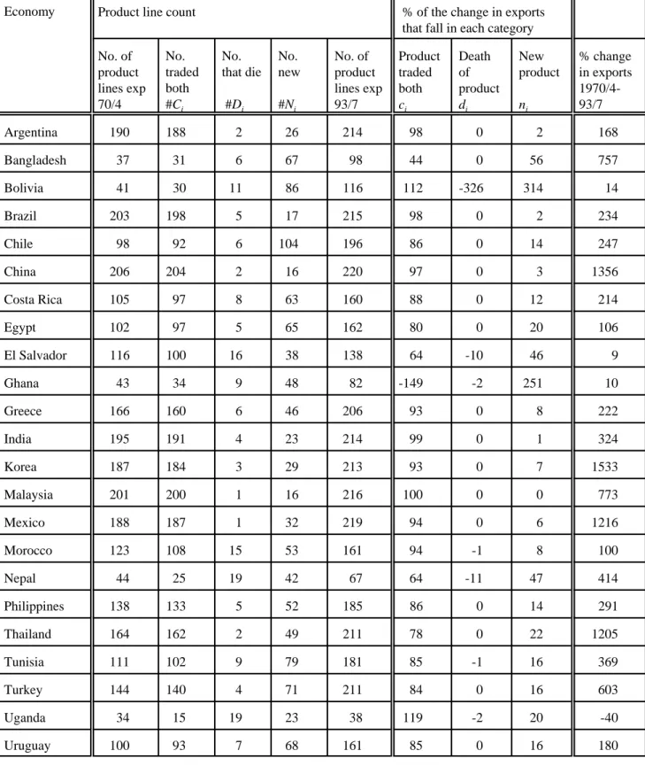
Table 1 reports results, for a cutoff value of $ = $50,000 pa. The left hand block of the table¯x reports numbers of product lines exported, and to the right of this we give the share of countries’ export growth falling in each of the categories. Thus, the decomposition for Argentina is as follows: of the 214 product lines (out of a maximum of 224) that were exported in 1993/97, 188 had been exported in 1970-74, and 26 were new; 2 of the product lines exported in 1970/74 ‘died’. Of Argentina’s overall real export growth of 168% during the period, 98% was in continuing product lines, c_i, 2% in new product lines n_i, while product lines that died, d_i, amounted to - 0.01% of the total export growth.

Looking down the table it is evident that only a few economies (Bangladesh, Bolivia, El Salvador, Ghana, and Nepal) experience substantial changes in the set of products that they export. Death of a product line is quite infrequent (with a $50,000 cutoff) and the volumes of trade loss associated with death of product lines is generally negligible. Birth of new products is more frequent, although the importance of new products to trade growth is modest.

The summary for the exports of all 23 countries is given in the left hand panel of table 2. These are the aggregates across exporting countries, 100_M_i_M_k₃_C and similarly for sets D_i and

iû

X_ik/_M_i ûX_i

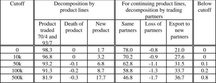
N_i. For our baseline cutoff of $50,000 we see that 93.2% of the growth of trade is in continuing product lines, while only a very small amount of exports are lost through the death of product lines. New products accounted for only 6.8% of observed export growth. Table 2 also reports the effects of using different cutoffs. The share of export growth attributable to the birth of new products is quite sensitive to this cutoff, and rises quite sharply, reaching 17.7% at a cutoff of $500,000 pa.

2.2 Decomposition by destination

(9)

in both 1970-4 and 1993-7 (the elements of sets C_i) we performed an additional decomposition to examine the extent to which the observed changes in export flows were accounted for by changes in trading partners. We define two more indicators that determine whether nation i exported product line k to nation j in 1970-4 and in 1993-7:

S X_ijk(70/4) ö 1 if X k ij(70/4)'¯x, 0 otherwise. S X_ijk(93/7) ö 1 if X k ij(93/7)'¯x, 0 otherwise.

To differentiate between those tuples (i, j, k) where the trading partners have changed and where they have not, define for each source country i and product line k the following three sets:

, D_ik 2 j | S X_ijk(70/4) ö1B S X_ijk(93/7) ö0

, N_ik 2 j | S X_ijk(70/4) ö0B S X_ijk(93/7) ö1 C_ik 2 j | S X_ijk(70/4) ö1B S X_ijk(93/7) ö1

Thus, D_ik is the set of countries to which country i stopped exporting good k. The value of the change in exports in this set can be calculated, and adding across product lines gives the change in country i exports associated with loss of trading partners. This number can be expressed relative to the change in country i ’s total exports to give d_iõ ö 100_M_k_M_j₃_Dk . Similarly, for

i û

X_ijk/ûX_i

products traded with new partners and with continuing partners, we write

, and . is therefore the value of

n_iõ ö 100_M_k_M_j₃_Nk i û

X_ijk/ûX_i c_iõ ö 100_M_k_M_j₃_Ck i û

X_ijk/ûX_i n_iõ

country i’s exports of long standing product lines to new partners, expressed as a percentage of country i’s overall export growth.

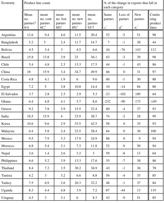
This second decomposition, which recall is only applied to goods k that were exported by nation i in both 1970-4 and 1993-7, is reported in table 3. The left hand block gives the average (across product lines) number of export partners of each country. This number typically increases significantly across the period. For example, Argentina’s mean number of partners increased from

(10)

11

The fact that Mexico and Nepal both export a high proportion of their respective exports to large neighbours may well account for this finding.

12.6 to 20.4. There is also some loss of partners, implying a substantial number of new partners % an average of 11.3 for Argentina. For 18 of the 23 countries the mean number of new partners exceeds the mean number for 1970/4.

Proportions of the change in the value of exports associated with these changes in partners are given in the right hand block of table 3. In Argentina’s case c_iõ = 52, d_iõ = -5, and n_iõ = 51; these numbers are for continuing product-lines, so sum to the share of Argentina’s export growth in continuing product lines given in the right hand column of the table. Thus, for Argentina, 51 per cent of the observed increase in Argentina’s total exports was accounted for by foreign sales of goods that (i) were exported at the beginning and the end of the sample and (ii) were exported to trading partners in 1993-7 that did not receive such exports in 1970-4. In other words, over half of Argentina’s export growth can be accounted for by this proliferation of trading partners.

Looking across countries, the share of export growth that can be attributed to sales of existing product lines to new trading partners in sizeable. In only three countries (Mexico, Nepal and Uganda) does the geographic spread of exports in long-standing product lines account for less than 25% of total export growth.11 The median share of export growth in our 23 economies that can be attributed to proliferation of export partners is 37 percent, and table 2 reports the share of the total export growth of all 23 countries that is attributable to exporting to new partners. At a $50,000 cutoff this is 31.5%, and raising the cutoff level increases this share to nearly 40%; even if the cutoff is set at zero it is still the case that 21% of export growth is attributable to reaching new partners. While these numbers are smaller than the share of export growth attributable to selling greater volumes to existing partners, they are nevertheless very substantial, and are the subject of econometric investigation in the next section.

(11)

12

In this section we drop the subscripts for source and product-line. Thus, for source i and product k, .

s_j(t) 2 S X_ijk(t)

The preceding section showed that a substantial part of the growth in developing country exports arises from selling products to new export markets&filling in the zeros in the product line bilateral trade matrix. What economic forces drive this process? We address this question by looking separately at each country’s exports of each product line to different destinations.

The economic forces determining whether or not a market is supplied can be divided into four broad categories. The first are supply side factors: the comparative advantage, exchange rate and cost levels of the supplying country. Since our approach is to estimate separately for each supplier and product line, these factors only vary in the time dimension, and we capture them by time trends or dummies. The second are ‘between country’ factors: from gravity modelling, these include distance of the destination market from the source, and whether or not they share a common border or language. They vary in the cross-section, but not in the time dimension. Third, are destination market characteristics, reflecting demand for the product. We will work with two such measures, one being the overall size of the country’s imports, and the other being its revealed comparative advantage for the product under study. These measures vary both in the cross-section and time series. Finally, we hypothesis that there are experience effects. These operate both within the market (so can be captured by past supply to the market) and between markets % the spatial spillover effects from proximate markets that have been previously supplied. The next sub-section outlines a modelling approach to capture all these effects.

3.1 Model structure

If a particular source country exports a particular product to destination market j at time t we write s_j(t) = 1, while s_j(t) = 0 if this bilateral export flow is zero or below the cutoff value12. In a given year, the decision to supply an export market depends on the revenue net of operating costs that can be earned in the market, relative to the recurring fixed cost of supplying the market. We denote the potential flow of operating profit earned in destination market j at time t by R_j(t), and the fixed costs

(12)

s_j(t) ö

1 if r_j(t) ' f_j(t),

0 otherwise. (1)

F_j(t); or in logs, r_j(t), f_j(t). We therefore have,

Before outlining in detail the modelling of net revenues and costs, several general points about our approach need to be made. The net revenues earned in market j will, we suppose, depend on supplier country factors, between country factors and destination market characteristics. The fixed costs f_j(t) depends on experience gained in market j and in other markets that are in some sense proximate to j. Thus, in a world with K potential export destinations, it will generally be the case that f_j(t) = f_j (s₁(t-1), s₂(t-1),..., s_j(t-1),<, s_K(t-1); u_j(t-1)) where u_j(t-1) is some random shock. The form of the function f_j(<) is export destination-specific, because we hypothesise that it will depend strongly on experience gained in the destination country, s_j(t-1), while the influence of other countries will depend on their proximity to market j. These relationships could, in principle, create a complex system of stochastic difference equations, in which entry to one market changes the costs of selling to that and to other markets in the next period. Thus, exporting to Germany might provide experience in selling to (or information about) other European markets, making it more likely that the latter will be supplied in the next period. There is therefore a potential ‘bridgehead’ effect; with export growth being path dependent and exhibiting regional effects as sales spread from one country to others in close proximity.

The final general point about our approach is that we model export supply as a comparison of instantaneous benefits and costs, thereby ignoring forward-looking behaviour on the part of exporters. We have two reasons for making this assumption, the first of which is simplicity. Each exporter has number of state variables equal to the number of potential export markets and a shadow value (costate variable) for each market. This value equals the direct value of entering that market plus the value of spillover effects from entry (and spillover effects from markets that were entered because of the additional experience gained, and so on). This contrasts with the single state variable (to export or not) found in formulations by Roberts and Tybout (1997), amongst others. Essentially,

(13)

13

The exporter country under study is denoted i* and stripped out of this measure for reasons of

endogeneity.

the geographical issues on which we focus would, in a fully specified intertemporal model, increase the complexity of the problem by an order of magnitude. The other reason we ignore forward-looking behaviour is that we have product line, not firm level data. There is, therefore, no presumption that the spillover effects we identify in the data are internalised within the firm. In fact, our straightforward model is consistent with intertemporal optimising behaviour if experience effects are external to firms and each firm is small enough to ignore the effects of its actions on the aggregate stock of (product- and country-specific) experience. We therefore make the (not uncommon) assumption that each product line contains a large number of similar firms.

We now turn to looking in more detail at the determinants of net revenues and costs. Looking first at net revenues, supply country characteristics % such as the productivity of its export sector and its exchange rate -- are captured simply as a function of time. We denote these by E(t), and will represent them either by a time trend or time dummies. Between country effects include the proximity of country i to a potential export market j as measured by distance, the presence of a common border and whether businesses in both the exporter and the potential export destination use a common business language, so facilitating contracting and communication. We denote these three effects D_j, B_j and L_j respectively.

There are two main characteristics of the potential destination market. The first is its size, which we measure by its total imports (of all goods from all sources), m_j(t), expressed as the log of US dollar values. By working with imports we capture not just the economic size of the destination, but also its natural openness, trade policy, and bilateral exchange rate with the US dollar. The second market characteristic is its revealed comparative advantage in the product under study, as measured by the share of the product in its total imports, relative to the share of the product in world imports. Formally, we define z_jk(t) 2 _M_i_g_i_õ X_ijk(t) as country j’s imports of good k from all sources other than the exporter country under consideration.13_{Since we are looking at imports we define the} revealed comparative disadvantage of country j in good k at time t, RCD_jk(t), as

(14)

RCD_jk(t) ö z k j (t) /Mkz k j (t) Mjz k j (t) /MjMk z k j (t) (2) r_j(t) ö .₀ ø .₁m_j(t) ø .₂RCD_j(t) ø .₃D_j ø .₄B_j ø .₅L_j ø .₆E(t). ₍₃₎ f_j(t) ö 5₀ ø 5₁s_j(t÷1) ø 5₂P_j(t÷1)[1÷s_j(t÷1)] ø 5₃P_j(t÷1)s_j(t÷1) ø u_j(t÷1). ₍₄₎ Thus, for a particular product line under study, RCD_j(t) measures the extent to which country j’s imports are skewed towards the product, relative to the pattern of world imports as a whole. Pulling these elements together, we express revenue as:

Turning to fixed costs, our basic formulation is, in logarithmic form,

This expression has the following interpretation. The fixed cost of supplying market j depends on knowledge that has been gained about that market. The knowledge comes from two sources. One is previous experience in market j, as measured by the variable s_j(t-1). The other is spillovers from experience gained in related or proximate markets which we denote P_j(t-1). The importance of such spillovers is likely to depend on whether or not experience has been gained directly in market j, hence the interaction of the variable with s_j(t-1); if experience has not been gained, s_j(t-1) = 0, then

ù2 measures the value of the spillover. If market j experience has been already obtained directly, s_j(t-1) = 1, then the case for obtaining further knowledge through spillovers from other markets seems likely to be much reduced; we include the effect in any case, and it is measured by ù₃. Experience gained in related markets, variable P_j(t-1), depends on the economic proximity of market j to other export markets that were supplied at t-1. This is ‘proximity to the supply frontier’, which we measure in three different ways. The first proximity measure is a dummy for whether or not

(15)

f_j(t) ö 5₀ ø 5₁s_j(t÷1)ø5₂near1_j(t÷1)ø5₃near2_j(t÷1)ø5₄bord1_j(t÷1)ø5₅bord2_j(t÷1) ø5₆lang1_j(t÷1)ø5₇lang2_j(t÷1)øu_j(t).

(5) country j has a common border with a country that was supplied in the preceding period. Thus, if border_jk is the matrix of border dummies, with elements equal to 1 if and only if countries j and k share a common border, then, bord_j(t÷1) ö 1 if _M_kborder_jks_jk(t÷1) > 0, and zero otherwise. The second measure is a dummy variable for whether or not country j has a common business language with a country that was supplied in the preceding period. Proceeding as with the border measure, we construct lang_j(t-1). The third measure is based on geographical distance. Thus, near_j(t-1) measures the log distance from market j to the closest foreign market that was supplied in period t-1. Formally, near_j(t÷1)ö ÷min_k ln(dist_jk/dist_max) |s_k(t÷1)ö1 . dist_jk is distance from j to k, and we express it relative to the furthest distance between any pair of countries; for ease of interpretation of results we measure proximity rather than distance, hence the minus sign.

Each of these measures is interacted with market j experience, as already indicated in equation (4). As a matter of notation we use numbers 1 (and 2) to distinguish cases where market k was not (was) itself supplied in the preceding period. Thus, near1_j(t÷1) ö near_j(t÷1)[1÷s_j(t÷1)] and , and similarly for bord1_j(t-1), bord2_j(t-1) and lang1_j(t-1), near2_j(t÷1) ö near_j(t÷1) s_j(t÷1)

lang2_j(t-1). We anticipate that the spillover effects are strongest for markets that have not been previously supplied, so the variables dist1_j(t-1), bord1_j(t-1) and lang1_j(t-1) will be our primary interest in the results that follow.

Pulling these elements together equation (4) becomes

3.2 Data and estimation

To ensure comparability with the product-line decompositions described in section 2 we assembled, for each of the 23 developing economies, a panel dataset for each product line where exports to at least one trading partner exceeded a cutoff level, , here taken to be $50,000. For each product line,¯x

(16)

14

As is well known, when employing datasets with dichotomous dependent variables, there has to be a sufficient number of ones and zeros for the estimation routines to converge onto a set of parameter estimates. For this reason, a number of product-lines were dropped during estimation. In tables 5 and 6 we report the number of product-lines for which panel estimation was possible and there is a considerable variation across countries. For instance, only five of Uganda’s product lines were estimated, whereas 203 panels were estimated for China. The simple mean of the number of product lines estimated for our 23 countries was 105.96.

15

Grimes (1996) contains the base data on the languages used in business. However, a useful summary of this dataset can be found in tabular form at www.infoplease.com/ipa/A0774735.htm.

16

It is worth noting that in many countries the list of official languages is a subset of those used to conduct business.

we created the dichotomous dependent variable s_j(t) for each potential export destination j (of which there are 92 in our study) in each year, 1970-1997. As will become clear below, we drop the first year of data (1970) leaving each panel with 27 annual observations.14

Turning to the independent variables, we used the U.S. dollar value of a potential export destination’s total imports (of all goods from all sources) for m_j(t), data taken from the World Bank’s World Development Indicators. The measure RCD_j(t) was constructed, for each product line, from the NBER World Trade Database.

Our proxy for transportation costs is, following the gravity literature, the distance between the capital cities of the exporter and a potential overseas market, measured in log kilometres, dist_ij.. Our proxy for a common business language was constructed from a database on the fifty most widely-spoken languages in the world.15 Specifically, we assembled a dataset for our 23 exporting nations and our 92 potential export destinations that indicate whether English, French, German, Spanish, Portuguese, or Mandarin Chinese are commonly used business languages in each economy.16 Our proxy for language_ij was based on whether or not an export destination and an exporter both used any one of these six languages for business purposes.

In the absence of product-line data on productivity, wage, and costs for all 23 economies, we employed two types of proxies for E_j(t), the time-varying supply side characteristics of the exporter, the first of which is simply a time trend, denoted by t.

(17)

s_j(t) ö .₀ø.₁m_j(t)ø.₂RCD_jø.₃D_jø.₄B_jø.₅L_jø.₆tø5₁s_j(t÷1)ø5₂near1_j(t÷1)ø

5₃near2_j(t÷1)ø5₄bord1_j(t÷1)ø5₅bord2_j(t÷1)ø5₆lang1_j(t÷1)ø5₇lang2_j(t÷1)øu_j(t). (6)

s_j(t) ö .₀ø.₁m_j(t)øK_jøT(t)ø5₁s_j(t÷1)ø5₂near1_j(t÷1)ø5₃near2_j(t÷1) ø54bord1j(t÷1)ø55bord2j(t÷1)ø56lang1j(t÷1)ø57lang2j(t÷1)øuj(t).

(7) Combining the elements of the revenue and cost functions gives an estimating equation of the form:

The presence of the lagged dependent variable requires truncation of each panel from 28 years to 27 years in length. As no attempt is made to include export-destination fixed effects in this specification, straightforward logistic estimation was used to estimate the parameters.

Equation (6) provides the benchmark specification, and we estimate it by standard logit methods. We also believe that there may be both country and time fixed effects that are not captured in this specification. First, the supply side changes in the exporting nation, as well as bilateral exchange rate changes, are likely to be better captured with time dummies than with a time trend. Thus, we replace the time trend by a full set of time dummies, T(t). Second, export destination-specific effects are likely to influence the dependent variable. To the extent that these effects are time invariant (such as climate and, to a lesser extent, governance) then they can be captured by fixed effects. We therefore also include country fixed effects, K_j; these obviously replace time invariant country characteristics, giving estimating equation of the form,

Incorporating the country fixed effects, however, creates problems in panels with dichotomous dependent variables. As Anderson (1973), Chamberlain (1980), and Hsiao (1986) have demonstrated, logit estimation with fixed effects generates inconsistent maximum likelihood estimates of both the fixed effects and the slope parameters. Fortunately, Anderson (1970, 1973) and McFadden (1974) have shown that the slope parameters (but not the fixed effects) can be consistently estimated using data on those "individuals" in the panel where the dependent variable

(18)

17

We have only begun to tackle the problems created by the inclusion of the lagged dependent variable. We have tried instrumenting for the latter and, for what it is worth, our preliminary finding is failure to instrument reduces the significance of the learning effects considered here.

switches value during the sample. We employ such conditional logit estimation here.17 3.3 Product-line estimation

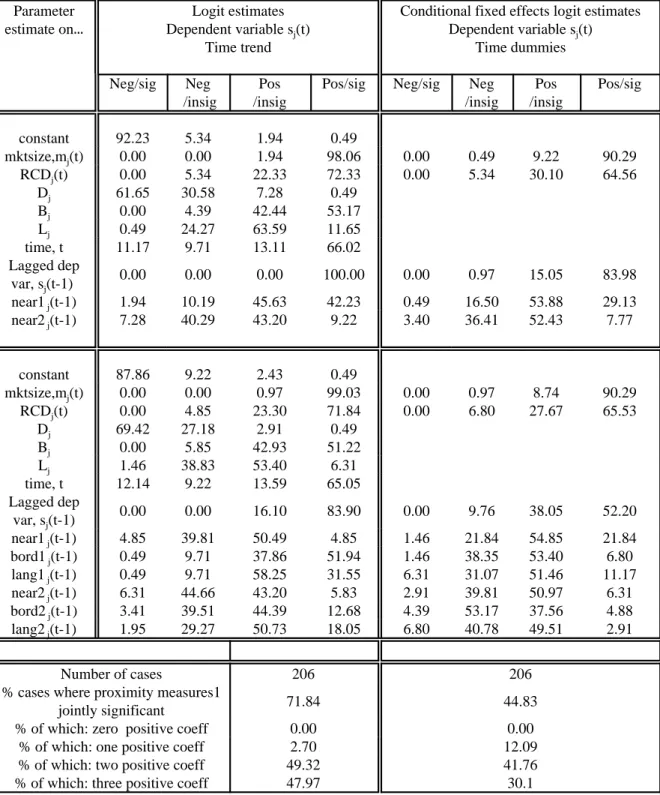
We present results for both the specifications (6) and (7). The base specification (6) has the advantage of revealing the role of the usual gravity variables (distance, border and language) as well as using more information, i.e. including observations for countries where the dependent variable does not change during the period. The base specification (which we refer to as the logit estimates) plus the conditional logit estimation of equation (7) result in over 4,000 sets of parameter estimates. To facilitate a discussion of the estimation results, we first present the findings for China (for whom the largest number of panels were estimated) in table 4. Then we present in tables 5 and 6 summaries of the findings for each of the 23 economies, focussing on the explanatory power of the three spillover effects identified earlier.

The top left and top right blocks of table 4 present the results of estimating our logit and conditional logit specifications, initially with only the distance measure of proximity to the supply frontier. We see that the market size variable m_j(t) is positive and statistically significant in 98.06 percent of China’s 203 product lines, or 90.29 percent once time invariant country fixed effects and time dummies are included. The revealed comparative advantage of each market is positive and statistically significant in around two-thirds of cases. Conventional exporter-to-importer distance is negative and statistically significant in more than half of cases, which, along with the market size parameter estimates, confirms the importance of two traditional "gravity variables." The presence of a common border between China and an export destination adds significantly to the probability of being supplied in over a half of cases. Hysteresis effects are strong, as evidenced by the fact that the lagged dependent variable is statistically significant in 100% of cases for the logit estimates, and more than 80% once fixed effects are included. Encouragingly, there are very few anomalous results&where the estimated parameter had the "wrong" sign and was statistically significant.

(19)

The variables measuring spillovers from presence in proximate markets, near1 and near 2 are in line with theoretical priors. They have a significant and positive impact in 30-40% of product lines where markets were not directly supplied in the previous period (near1). However, when the market was supplied in the previous year (near2), the spillover effect is positive and significant in only around 8-10% of product lines.

Remaining parts of table 4 report results when all the proximity to the frontier variables are included. Correlation between these variables reduces the proportion of cases in which any one is separately significant, and we report joint significance tests (Wald test) in the bottom part of the table. For the logit estimates the three effects near1, bord1 and lang1 are jointly significant in 71.8% of cases. The presence of country and time fixed effects reduces the number of Chinese product lines where these three mechanisms are jointly statistically significant, but even so, these effects remain significant in over 44 percent of product lines. Moreover, in every single product line at least one of the three learning mechanisms is estimated to have a positive coefficient and in the vast majority (97% logit, 72% conditional logit) two or more of these mechanisms have a positive coefficient. The Chinese parameter estimates, then, are supportive of the broad hypothesis that the path of her entry into overseas markets since 1970 has been influenced not only by traditional gravity variables, but also by spillover effects from existing foreign markets, especially those which are geographically close to those foreign markets that are currently supplied.

Looking at each of the proximity to the supply frontier measures separately, we see that each is significant in a proportion of cases, although their relative significance varies between the logit and conditional logit estimates. As we look at other countries, it is generally the case the geographical distance is the most important mechanism, followed by common border and language.

Results for other countries are given in appendix table 2, and results for all countries are summarised in Tables 5 and 6. The joint significance of these three proximity measures is reported on a country-by-country basis in table 5. The logit estimates indicate that in nearly half of cases the spillover

(20)

18

The raw correlation coefficient between the growth of exports and proportion of product lines where spillover effects are jointly significant is 21% for the conditional logit estimates and 12% for the logit estimates.

effects are significant. In the most conservative parameter estimates (the conditional logit estimates including time and country fixed effects) suggest that in 25% percent of product lines these spillover effects have contributed to market entry. Countries with the lowest proportion of jointly significant effects are Tunisia, Nepal, and (according to the conditional logit estimates Egypt and Uganda). Interestingly, there is a positive correlation between the overall rate of growth of countries’ exports over the period and the proportion of their product lines for which learning effects are significant.18 Table 6 looks at each of the proximity measures separately. We see that for the logit estimates border effects are the most important measure of proximity, while for the conditional logits the distance measure becomes the most important. In some 14.4% of cases the geographical distance to the supply frontier has a positive and significant effect on the probability of a market receiving exports.

4. Conclusions

The literature on the determination of bilateral trade flows has paid little attention to the falling number of zeros in bilateral trade matrices that has been occurred since 1970. This phenomenon --which we call the geographic spread of exports -- is important as the trade flows associated with it alone account for one third of developing economies’ export growth since 1970, a fact we document here for 23 developing countries.

Naturally, much of the this spread is driven by supply side improvements in exporting countries, which we model as depending simply on time. But what determines which markets are entered? We show that it depends on three sorts of factors. One is market demand, measured both by overall import demand and by destination markets’ revealed comparative advantage in the product. The second is distance from the supplier, measured by great circle distance, and sharing a common

(21)

border or language. The third is experience gained, both in the destination market and from previous exports to proximate markets. These effects are significant in between 25% and 50% of cases studied. Thus, if, say, China has exported a particular product line to Germany, this raises the probability that it will come to export to countries close to Germany. Of course countries close to Germany share, with Germany, a similar distance from China, and possibly also similar comparative advantage and market size. However, even controlling for these factors we find the spillover effects from supplying proximate markets to be significant.

The presence of these spatial spillovers leaves open the question of exactly what mechanism is driving them. Learning effects are one likely candidate, although we cannot identify these separately from the effects of sunk investments in regional distribution networks. We show, however, that proximity effects operate most often through pure distance, rather than through either border effects or shared language effects.

In a sense our findings bode well for the future prospects for developing economies’ exports. The findings suggest that there are costs of entering markets, but once overcome there is persistence of presence in the market, and entering related markets becomes more likely. Both geography and history matter in shaping which markets are supplied, but hysteresis and experience effects suggest a ratchet-like outcome, in which continuing export growth can be sustained

(22)

References

Anderson, E. B. 1970. "Asymptotic properties of conditional maximum likelihood estimators," Journal of the Royal Statistical Society, B32: 283-301.

Anderson, E.B. 1973. Conditional Inference and Models for Measuring. Copenhagen: Mentalhygieniejuisk Forlag.

Anderson, James, and Eric Van Wincoop. 2001. "Gravity with Gravitas: A Solution to the Border Puzzle." National Bureau of Economic Research Working Paper number 8079. Cambridge, MA.

Baier, Scott, and Jeffrey Bergstrand. 2001. "The Growth of World Trade: Tariffs, Transport Costs, and Income Similarity." Journal of International Economics 53(1): 1-27.

Bernard, Andrew, and J. Bradford Jensen. 2001. "Why some firms export." National Bureau of Economic Research working paper number 8349.

Chamberlain, G. 1980. "Analysis of Covariance in Qualitative Data," Review of Economic Studies, 47: 225-238.

Cheng, Leonard K., and Henryk Kierzkowski (eds). 2000. Global Production and Trade in East Asia. Kluwer Academic Publishers.

Clerides, Sofronis, Saul Lach, and James R. Tybout. 1998. "Is ‘learning by doing’ important? Mirco-dynamic evidence from Colombia, Mexico and Morocco." Quarterly Journal of Economics 96:1-58.

Das, Sanghamitra , Mark J. Roberts, and James R. Tybout. 2001. "Market Entry Costs, Producer Heterogeneity, and Export Dynamics." National Bureau of Economic Research working paper number 8629.

Feenstra, Robert C., Robert E. Lipsey, and Harry P. Bowen.1997. "World Trade Flows, 1970-1992, with Production and Tariff Data." National Bureau of Economic Research working paper number 5910.

(23)

Estimation." Paper prepared for the Special Issue of the Scottish Journal of Political Economy on the Gravity Equation.

Flam, Harry, and Elhanan Helpman. 1987. "Vertical Product Differentiation and North-South Trade," American Economic Review 77:810-822

Grimes, Barbara F. (ed.) 1996. Ethnologue. Thirteenth edition. Summer Institute of Linguistics, Inc. Grossman, Gene, and Elhanan Helpman. 1989. "Product development and international trade."

Journal of Political Economy 97: 1261-1283.

Grossman, Gene, and Elhanan Helpman. 1991. "Quality ladders and product cycles." Quarterly Journal of Economics 106: 557-586.

Grossman, Gene, and Elhanan Helpman. 1991. "Endogenous product cycles." Economic Journal 101: 1214-1229.

Haveman, Jon, and David Hummels. 2001. "Alternative Hypotheses and the Volume of Trade: the Gravity Equation and the Extent of Specialization." CIBER working paper number 2000-004. Purdue University.

Harrigan, James. 2001. "Specialization And The Volume Of Trade: Do They Obey The Laws?" National Bureau of Economic Research Working Paper number 8675. Cambridge, MA. Hsiao, Cheng. 1986. Analysis of Panel Data. New York: Cambridge University Press.

Krugman, Paul K. 1995. "Growing World Trade: Causes and Consequences." Brookings Papers on Economic Activity 1: 327-377.

Matsuyama, Kiminori. 2000. "A Ricardian Model with a Continuum of Goods under Nonhomothetic Preferences: Demand Complementarities, Income Distribution, and North-South Trade." Journal of Political Economy 108(6): 1093-1120.

McFadden, Daniel. 1974. "The Measurement of Urban Travel Demand." Journal of Public Economics, 3: 303-328.

McKendrick, David G., Richard F. Doner, and Stephan Haggard. 2000. From Silicon Valley to Singapore: Location and Competitive Advantage in the Hard Disk Drive Industry. Stanford

(24)

University Press.

Rauch, James E. 1996. "Trade and Search: Social Capital, Sogo Shosha, and Spillovers," National Bureau of Economic Research working paper number 5618.

Rauch, James E. 1999. "Networks versus Markets in International Trade." Journal of International Economics, 48: 7-35.

Rauch, James E. 2001. "Business and Social Networks in International Trade." Journal of Economic Literature.

Redding, Stephen, and Anthony J. Venables. 2000. "Economic Geography and International Inequality." Centre for Economic Policy Research Discussion Paper number 2568. London, United Kingdom.

Roberts, Mark J., and James R. Tybout. 1997. "The decision to export in Colombia: an empirical model of entry with sunk costs." American Economic Review 87: 545-64.

Schott, Peter K. 2001. "One Size Fits All? Heckscher-Ohlin Specialization in Global Production." National Bureau of Economic Research working paper number 8244.

Stokey, Nancy L. 1991. "The Volume and Composition of Trade between Rich and Poor Countries." Review of Economic Studies 58(1): 63-80.

Vernon, Raymond. 1966. "International Investment and International Trade in the Product Cycle." Quarterly Journal of Economics 80: 190-207.

(25)

Table 1: Export growth decompositions by product-line.

Economy Product line count % of the change in exports

that fall in each category No. of product lines exp 70/4 No. traded both #Ci No. that die #Di No. new #Ni No. of product lines exp 93/7 Product traded both ci Death of product di New product ni % change in exports 1970/4-93/7 Argentina 190 188 2 26 214 98 0 2 168 Bangladesh 37 31 6 67 98 44 0 56 757 Bolivia 41 30 11 86 116 112 -326 314 14 Brazil 203 198 5 17 215 98 0 2 234 Chile 98 92 6 104 196 86 0 14 247 China 206 204 2 16 220 97 0 3 1356 Costa Rica 105 97 8 63 160 88 0 12 214 Egypt 102 97 5 65 162 80 0 20 106 El Salvador 116 100 16 38 138 64 -10 46 9 Ghana 43 34 9 48 82 -149 -2 251 10 Greece 166 160 6 46 206 93 0 8 222 India 195 191 4 23 214 99 0 1 324 Korea 187 184 3 29 213 93 0 7 1533 Malaysia 201 200 1 16 216 100 0 0 773 Mexico 188 187 1 32 219 94 0 6 1216 Morocco 123 108 15 53 161 94 -1 8 100 Nepal 44 25 19 42 67 64 -11 47 414 Philippines 138 133 5 52 185 86 0 14 291 Thailand 164 162 2 49 211 78 0 22 1205 Tunisia 111 102 9 79 181 85 -1 16 369 Turkey 144 140 4 71 211 84 0 16 603 Uganda 34 15 19 23 38 119 -2 20 -40 Uruguay 100 93 7 68 161 85 0 16 180

(26)

Table 2: Export growth decompositions for entire 23 country sample.

Percentage of the change in export values (all 23 countries) that fall in each category. Various cutoffs.

Cutoff Decomposition by

product lines

For continuing product lines, decomposition by trading partners Below cutoff Product traded 70/4 and 93/7 Death of product New product Same partners Loss of partners Export to new partners 0 98.3 0 1.7 78.0 -0.8 21.0 0 10k 96.8 0 3.2 70.2 -0.9 27.6 0 50k 93.2 -0.1 6.8 62.8 -1.1 31.5 0.1 100k 91.3 -0.2 8.7 58.8 -1.3 33.7 0.2 500k 81.9 -0.3 17.7 46.8 -1.7 36.7 0.8

(27)

Table 3: Export growth decompositions by partner

Economy Product line count % of the change in exports that fall in

each category Mean no. partnrs7 0/4 mean no. cont partnrs #Ci k mean no. lost partnrs #Di k mean no. new partnrs #Ni k mean no. partnrs 93/7 Same partnrs ci * Loss of partnrs di * New partnrs ni * Contin uing product lines Argentina 12.6 9.4 4.6 11.5 20.4 52 -5 51 98 Bangladesh 5.2 5 2.4 11.7 14.7 7 -1 38 44 Bolivia 4.5 3.4 3 4.5 6.6 44 -76 143 112 Brazil 15.8 13.8 3.9 23 36.1 63 -3 39 98 Chile 5.4 4.8 2.3 13.3 17.5 44 -1 43 86 China 18 15.9 3.4 34.7 49.9 66 0 31 97 Costa Rica 4.8 4.1 1.9 6 9.6 60 -1 30 88 Egypt 7.2 5 3.8 10.8 14.4 10 -14 84 80 El Salvador 3.7 2.8 2.3 2.9 5.3 -23 -102 189 64 Ghana 6.4 4.8 4.1 5.7 8.6 -232 -90 173 -149 Greece 9.2 7.8 2.9 15.5 22.4 60 -4 37 93 India 18.5 15.9 4 23.9 38.7 74 -2 28 99 Korea 10.6 9.6 2.9 33.5 42.5 58 0 35 93 Malaysia 6.4 5.8 2.4 23.5 28.4 64 0 36 100 Mexico 9.5 7.9 3.3 17.9 24.9 86 0 9 94 Morocco 6.8 5.4 3.1 7.3 11.8 52 -9 50 94 Nepal 2.6 1.4 2.6 3.2 3 59 -8 13 64 Philippines 6.6 5.2 3.9 13.3 17.6 55 -7 38 86 Thailand 8.4 7.2 3.5 30.2 36.9 43 -1 36 78 Tunisia 4.2 3 3.2 6.6 8.8 56 -4 33 85 Turkey 7.5 6.9 2.6 26.3 32.2 48 -1 37 84 Uganda 8.3 4.4 4.8 3.9 7.2 -87 -44 13 119 Uruguay 4.3 3 3.1 6 8.3 43 -9 51 85

(28)

Table 4: Estimation results for China

Proportion of product lines for which estimated coefficient falls into each sign and significance category. Parameter estimate on< Logit estimates Dependent variable sj(t) Time trend

Conditional fixed effects logit estimates Dependent variable sj(t) Time dummies Neg/sig Neg /insig Pos /insig

Pos/sig Neg/sig Neg

/insig Pos /insig Pos/sig constant 92.23 5.34 1.94 0.49 mktsize,mj(t) 0.00 0.00 1.94 98.06 0.00 0.49 9.22 90.29 RCDj(t) 0.00 5.34 22.33 72.33 0.00 5.34 30.10 64.56 Dj 61.65 30.58 7.28 0.49 Bj 0.00 4.39 42.44 53.17 Lj 0.49 24.27 63.59 11.65 time, t 11.17 9.71 13.11 66.02 Lagged dep var, sj(t-1) 0.00 0.00 0.00 100.00 0.00 0.97 15.05 83.98 near1 j(t-1) 1.94 10.19 45.63 42.23 0.49 16.50 53.88 29.13 near2 j(t-1) 7.28 40.29 43.20 9.22 3.40 36.41 52.43 7.77 constant 87.86 9.22 2.43 0.49 mktsize,mj(t) 0.00 0.00 0.97 99.03 0.00 0.97 8.74 90.29 RCDj(t) 0.00 4.85 23.30 71.84 0.00 6.80 27.67 65.53 Dj 69.42 27.18 2.91 0.49 Bj 0.00 5.85 42.93 51.22 Lj 1.46 38.83 53.40 6.31 time, t 12.14 9.22 13.59 65.05 Lagged dep var, sj(t-1) 0.00 0.00 16.10 83.90 0.00 9.76 38.05 52.20 near1 j(t-1) 4.85 39.81 50.49 4.85 1.46 21.84 54.85 21.84 bord1 j(t-1) 0.49 9.71 37.86 51.94 1.46 38.35 53.40 6.80 lang1 j(t-1) 0.49 9.71 58.25 31.55 6.31 31.07 51.46 11.17 near2 j(t-1) 6.31 44.66 43.20 5.83 2.91 39.81 50.97 6.31 bord2 j(t-1) 3.41 39.51 44.39 12.68 4.39 53.17 37.56 4.88 lang2 j(t-1) 1.95 29.27 50.73 18.05 6.80 40.78 49.51 2.91 Number of cases 206 206

% cases where proximity measures1

jointly significant 71.84 44.83

% of which: zero positive coeff 0.00 0.00

% of which: one positive coeff 2.70 12.09

% of which: two positive coeff 49.32 41.76

(29)

Table 5: Country-by-country summary of joint significance of learning mechanisms.

Economy Number of product lines

estimated

Percentage of product lines where near1, bord1, and lang1 are jointly significant

Percentage of product lines where no learning dynamic

was positive Logit estimation Conditional logit estimation Logit estimation Conditional logit estimation Argentina 174 55.75 21.84 0.00 0.00 Bangladesh 26 42.31 23.08 9.09 0.00 Bolivia 15 26.67 26.67 0.00 0.00 Brazil 187 57.75 29.95 1.85 3.57 Chile 123 40.65 20.33 2.00 0.00 China 206 71.84 30.10 0.00 0.00 Costa Rica 78 41.10 21.62 0.00 0.00 Egypt 70 48.57 14.29 2.94 0.00 El Salvador 36 51.72 21.88 0.00 14.29 Ghana 17 82.35 29.41 0.00 0.00 Greece 160 47.50 20.63 0.00 6.06 India 186 43.55 35.48 0.00 0.00 Korea 182 62.09 24.73 0.00 0.00 Malaysia 179 34.64 33.52 8.06 5.00 Mexico 176 43.75 25.00 0.00 2.27 Morocco 74 44.59 27.03 0.00 0.00 Nepal 16 31.25 18.75 0.00 0.00 Philippines 131 38.17 22.90 6.00 0.00 Thailand 176 36.93 22.73 0.00 2.50 Tunisia 74 22.97 14.86 5.88 27.27 Turkey 158 60.13 18.35 0.00 0.00 Uganda 7 42.86 14.29 0.00 0.00 Uruguay 58 60.34 27.59 0.00 0.00 Simple mean 109.09 47.28 23.70 1.56 2.65 Weighted mean 48.97 25.06 1.47 2.35

(30)

Table 6: Country-by-country summary of statistical significance of different learning mechanisms. Exporter Number of product lines estimated Logit estimation, percentage of product lines with positive and statistically

significant coefficients for

Conditional logit estimation, percentage of product lines with

positive and statistically significant coefficients for

near1 bord1 lang1 near1 bord1 lang1

Argentina 174 9.77 45.98 9.20 11.49 8.05 5.75 Bangladesh 26 1154 19.23 7.69 3.85 11.54 3.85 Bolivia 15 667 20.00 0.00 0.00 6.67 0.00 Brazil 187 14.97 21.93 25.67 15.51 8.02 9.09 Chile 123 1463 21.14 0.81 10.57 4.07 5.69 China 206 485 51.94 31.55 21.84 6.80 11.17 Costa Rica 78 3590 3.85 2.74 15.38 6.41 2.70 Egypt 70 1286 30.00 18.57 1000 8.57 2.86 El Salvador 36 3611 2.78 3.45 13.89 8.33 0.00 Ghana 17 5294 29.41 0.00 17.65 11.76 0.00 Greece 160 1375 15.63 20.00 9.38 8.75 3.75 India 186 1613 26.88 4.30 23.66 11.83 10.22 Korea 182 1593 17.58 37.36 14.84 10.44 5.49 Malaysia 179 1061 13.41 2.79 16.76 8.94 12.29 Mexico 176 682 34.09 9.09 15.34 6.25 2.84 Morocco 74 1892 18.92 8.11 10.81 8.11 6.76 Nepal 16 3750 6.25 6.25 12.50 0.00 0.00 Philippines 131 21.37 6.11 3.82 14.50 2.29 4.58 Thailand 176 13.07 10.80 11.93 14.77 5.11 7.39 Tunisia 74 13.51 5.41 6.76 1.35 4.05 2.70 Turkey 158 22.15 20.89 36.08 11.39 10.13 4.43 Uganda 7 57.14 0.00 14.29 14.29 14.29 14.29 Uruguay 58 24.14 29.31 3.45 15.52 3.45 6.90 Simple mean 109.09 20.49 19.63 11.47 12.84 7.56 5.34 Weighted mean 15.22 23.08 14.96 14.43 7.57 6.46

(31)

Appendix 1: List of Potential Export destinations.

Algeria Finland Malaysia Spain

Argentina France Mali Sri Lanka

Australia Gabon Mauritius Sudan

Austria Germany Mexico Sweden

Bangladesh Ghana Morocco Switzerland

Belgium (includes Luxembourg)

Greece Myanmar (formerly

Burma)

Syrian Arab Republic

Benin Guatemala Nepal Taiwan

Bolivia Haiti Netherlands Tanzania

Brazil Honduras New Zealand Thailand

Burkina Faso Hong Kong Nicaragua Trinidad and Tobago

Cameroon India Nigeria Tunisia

Canada Indonesia Norway Turkey

Chile Iran Oman Uganda

China Ireland Pakistan United Arab Emirates

Colombia Israel Panama United Kingdom

Congo, Republic of Italy Papua New Guinea United States of

Costa Rica Jamaica Paraguay Uruguay

Cote d'Ivoire Japan Peru Venezuela

Denmark Jordan Philippines Zaire (now Democratic

Republic of the Congo)

Dominican Republic Kenya Portugal Zambia

Ecuador Korea, Republic of

(South)

Saudi Arabia Zimbabwe

Egypt Kuwait Senegal

El Salvador Madagascar Singapore

Ethiopia (includes Eritrea)

(32)

Appendix Two: Country-By-Country Econometric Estimates

Argentina

Logit estimates

Dependent variable sj(t)

Other independent variables: mj(t), RCDj(t), Dj, Bj, Lj , time trend

Conditional logit estimates Dependent variable sj(t)

Other independent variables: mj(t), RCDj(t) , time dummies

Neg/sig Neg/insig Pos/insig Pos/sig Neg/sig Neg/insig Pos/insig Pos/sig

lagdep 0.00 1.72 19.54 78.74 0.00 14.94 62.64 22.41 near1 9.20 49.43 31.61 9.77 2.87 33.91 51.72 11.49 bord1 0.57 10.92 42.53 45.98 2.87 31.03 58.05 8.05 lang1 7.47 38.51 44.83 9.20 3.45 39.08 51.72 5.75 near2 20.69 42.53 29.89 6.90 0.57 35.63 54.02 9.77 bord2 2.87 23.56 53.45 20.11 3.45 35.63 54.02 6.90 lang2 12.90 43.23 38.06 5.81 2.37 45.56 48.52 3.55 Number of cases 174 174

% cases where proximity

measures1 jointly significant 55.75 21.84

% of which: zero positive coeff 0 0

% of which: three positive coeff 19.59 28.95

Bangladesh

Logit estimates

Other independent variables: mj(t), RCDj(t), Dj, Bj, Lj time trend

lagdep 0 7.69 46.15 46.15 0.00 30.77 42.31 26.92 near1 19.23 42.31 26.92 11.54 7.69 46.15 42.31 3.85 bord1 0.00 15.38 65.38 19.23 3.85 34.62 50.00 11.54 lang1 11.54 42.31 38.46 7.69 3.85 15.38 76.92 3.85 near2 7.69 46.15 46.15 0.00 11.54 42.31 38.46 7.69 bord2 3.85 30.77 53.85 11.54 7.69 23.08 50.00 19.23 lang2 16.67 41.67 33.33 8.33 3.85 26.92 61.54 7.69 Number of cases 26 26

(33)

Bolivia

Logit estimates

Brazil

Logit estimates

(34)

Chile

Logit estimates

China

Logit estimates

(35)

Costa Rica

Logit estimates

lagdep 0.00 12.82 38.46 48.72 3.85 20.51 50.00 25.64 near1 1.28 17.95 44.87 35.90 1.28 34.62 48.72 15.38 bord1 15.38 53.85 26.92 3.85 6.41 43.59 43.59 6.41 lang1 10.96 34.25 52.05 2.74 1.35 48.65 47.30 2.70 near2 5.13 25.64 37.18 32.05 2.56 44.87 44.87 7.69 bord2 8.97 46.15 37.18 7.69 5.13 41.03 50.00 3.85 lang2 17.86 50.00 28.57 3.57 2.17 41.30 52.17 4.35 Number of cases 78 78

Egypt

Logit estimates