Sampling techniques and weighting procedures
for complex survey designs
–
The school cohorts of the National
Educational Panel Study (NEPS)
Dissertation
Presented to the Faculty for Social Sciences, Economics, and
Business Administration at the University of Bamberg
in Partial Fulfillment of the Requirements for the Degree of
DOCTOR RERUM POLITICARUM
by
Hans Walter Steinhauer, Diplom Volkswirt
born January 26, 1984 in Kaiserslautern, Germany
Date of Submission
June 5, 2014
Reviewers: Professor Mick P. Couper, PhD
University of Michigan, United States of America Professor Dr. Mark Trappmann
University of Bamberg, Germany Date of submission: June 5, 2014
The National Educational Panel Study (NEPS) set up a panel cohort of stu-dents starting in grade 5 and grade 9. To realize the corresponding samples of students NEPS applied a complex stratified multi-stage cluster sampling approach. To allow for generalizations from the sample to the universe es-pecially aspects of complex sample designs have to be considered and are reflected by design weights.
When applying multi-stage sampling approaches unit nonresponse, that is, units refuse to participate, may occur on each stage where decisions to-wards participation are made. To correct for potential bias induced by re-fusals of schools and students the derived design weights need to be ad-justed. Since participation decisions differ in many ways, for example by stage (school- or student-level), time (in the forerun of or during the panel) or reasons (school-level: workload or participation in other studies, student-level: not interested in the study, resentment to testing), design weights need to be carefully adjusted to reflect the participation decisions made on each stage properly. Participation decisions on the school level take informa-tion from sampling and the school recruitment process into account and are modeled using binary probit models with random intercept considering the federal-state-specific recruitment.
Schools participating are subsampled providing access to students in grade 5 and 9. Subsampling within schools provides a sample of two classes if at least three are present, otherwise all classes are selected. In creating de-sign weights this subsampling needs again to be incorporated in the weights. The students decision process on the next stage has to be accounted for in providing unit nonresponse adjusted weights. These decision processes take clustering at the school level as well as information on the initial sample, that is, respondents and nonrespondents, into account. The resulting net sample forms the panel cohorts of students in grade 5 and 9.
Based on the panel cohorts each student can again decide whether to participate or not for each successive wave. Providing additional informa-tion obtained in a parental interview with one parent this multi-informant perspective makes consideration of an additional participation decision nec-essary. Since participation decisions of a student and a parent are unlikely independent they should be modeled appropriately using bivariate models. To again account for a cluster structure these models are extended with a random intercept on the school level.
All these aspects of complex sample and survey designs as well as the different participation decisions involved need to be considered in weighting adjustments. The results point at typical characteristics influencing
partic-ipation decisions of schools, students and parents. Besides that the results stress the need to account for sample design and the nature of decision pro-cesses involved resulting in the actual participation.
Basis for this thesis
Earlier papers
This thesis is in parts based on work published in earlier papers by
• Aßmann et al. (2011),
• Aßmann, Steinhauer, and Rässler (2012),
• Steinhauer, Blossfeld, and Maurice (2012),
• as well as supplements of the data manuals accompanying the Scientific Use Files of the Starting Cohorts 3 (Grade 5 students) and Starting Cohort 4 (Grade 9 students) of the NEPS.
Data used
This thesis uses data from the National Educational Panel Study (NEPS). Results presented in this thesis are based on data mostly available as scientific use files. The corresponding data sets are:
• Starting Cohort 3 – Grade 5 (Paths through Lower Secondary School - Education Pathways of Students in 5th Grade and Higher)
DOI:10.5157/NEPS:SC3:1.0.0 DOI:10.5157/NEPS:SC3:2.0.0
• Starting Cohort 4 – Grade 9 (School and Vocational Training - Educa-tion Pathways of Students in 9th Grade and Higher)
DOI:10.5157/NEPS:SC4:1.1.0.
The NEPS data collection is part of the Framework Programme for the Pro-motion of Empirical Educational Research, funded by the German Federal Ministry of Education and Research and supported by the Federal States.
Statistical software used
All analysis provided are based on The R Project for Statistical Computing (R Core Team, 2014). See Appendix E for further information.
Contents
List of Figures IX
List of Tables XI
1 Introduction 1
2 Reviewing sampling and weighting techniques 7
2.1 The sampling frame . . . 7
2.2 Sampling techniques . . . 8
2.2.1 Explicit Stratification . . . 10
2.2.2 Multistage and multistage cluster sampling . . . 12
2.2.3 Systematic and systematic unequal probability sampling 14 2.3 Design weights and their adjustment . . . 16
2.3.1 Sample weighting adjustment . . . 17
2.3.2 Population weighting adjustment . . . 20
3 Sampling grade 5 and grade 9 students 23 3.1 Population . . . 23
3.2 Summarizing sampling for school cohorts . . . 25
3.3 Planning samples for school cohorts . . . 27
3.3.1 Sample design . . . 27
3.3.2 Determining the measure of size . . . 27
3.3.3 Determining the first stage sample size . . . 31
3.3.4 Replacing nonparticipating schools . . . 33
3.4 Sampling for grade 9 . . . 35
3.5 Sampling for grade 5 . . . 36
4 Weighting adjustments 41 4.1 Decision processes involved . . . 41
4.2 Frameworks for decision modeling . . . 44
4.3 Adjusting design weights for nonresponse . . . 49
4.3.1 Adjusting for nonparticipation on the institutional level 49 4.3.2 Adjusting for nonparticipation on the individual level . 51
4.4 Adjustments of the panel cohort for successive waves . . . 55
5 Weighting multi-informant surveys in institutional contexts 61 5.1 Students and parents participation decisions . . . 62
5.2 Model specifications for decision modeling . . . 64
5.2.1 Univariate probit model . . . 65
5.2.2 Bivariate probit model . . . 67
5.2.3 Parameter estimation . . . 70
5.2.4 Simulation based evaluation . . . 74
5.3 Application in grade 5 – re-weighting students and parents . . 77
6 Concluding remarks 83 6.1 Summary . . . 83
6.2 Critical assessment . . . 84
6.2.1 Complex sampling designs . . . 84
6.2.2 Modeling unit nonresponse and weighting adjustments 85 6.3 Outlook and future Research . . . 86
References 88
A List of Abbreviations and Nomenclature 99
B Tables 105
C Illustrating the GHK-simulator 119
D R code 123
List of Figures
1.1 The multicohort sequence design of the National Educational Panel Study. . . 2
2.1 Explicit stratification of schools by color of the school building. 11 2.2 Two-stage cluster sampling. . . 13 2.3 Systematic selection of units with random start. . . 15 2.4 Graphical illustration forpps sampling. . . 16
3.1 Changes from school year 2007/08 to 2008/09 for certain char-acteristics . . . 28 3.2 Inclusion probabilities for different scenarios . . . 30
4.1 Flowchart of decision processes ranging from the population to the panel cohort. . . 42 4.2 Participation patterns for panel cohort members. . . 56
C.1 Bivariate normal distribution and its’ marginal distribution. . 120
List of Tables
2.1 Example for systematic probability proportional to size sam-pling. . . 15 2.2 Example for cell weighting. . . 19
3.1 Population of regular schools by school type and schools pro-viding classes in grades 5 and 9 (school year 2008/09). . . 24 3.2 Population of Students in grade 5 and 9 by school type and
schools providing classes in grades 5 and 9 (school year 2008/09). 26 3.3 Allocation of first stage’s sample sizesmI. . . 33
3.4 Favorable samples. . . 34 3.5 Population sizes, sample sizes, and total measures of size for
schools with classes in grade 5 and 9 by strata. . . 37
4.1 Sampled vs. realized regular and special schools after replace-ment. . . 50 4.2 Distribution of participation rates per test group by starting
cohort. . . 52 4.3 Participation status of the initial sample by strata for SC3. . . 53 4.4 Participation status of the initial sample by strata for SC4. . . 54 4.5 Participation status for starting cohorts by wave. . . 57 4.6 Participation status by Starting Cohort and wave. . . 58
5.1 Participation statuses for students in SC3 and their parents by wave. . . 64 5.2 Statistical precision for R= 1000 replications. . . 75 5.3 Numerical precision forR = 1000 replications. . . 76
B.1 Distributions for net sample sizes nnet for different
participa-tion rates pby strata when sampling mI = 480 PSUs. . . 106
B.2 Schüler-Teilnahme-Liste / students participation list . . . 107 B.3 Results of random intercept models for school participation
(by strata). . . 108
B.4 Results of random intercept model for the participation of schools contacted for the supplement of migrants. Standard deviations are given in parentheses. . . 109 B.5 Models estimating the individual participation propensity used
to derive adjustment factors for sample weighting adjustment of the initial sample. . . 110 B.6 Models estimating the individual participation propensity used
to derive adjustment factors for sample weighting adjustment of wave 1 and 2, respectively. . . 111 B.7 Number of cases (n) and proportion (p) for variables in models
by wave. . . 112 B.8 lnL, AIC and BIC for considered model specifications. . . 113 B.9 Alternative models estimating the individual participation
propen-sity of students and parents for SC3 in wave 1. . . 114 B.10 Results for the bivariate probit models without and with
ran-dom intercept estimating the individual participation propen-sities for students and parents for SC3 in wave 1. . . 115 B.11 Alternative models estimating the individual participation
propen-sity of students and parents for SC3 in wave 2. . . 116 B.12 Results for the bivariate probit models without and with
ran-dom intercept estimating the individual participation propen-sities for students and parents for SC3 in wave 2. . . 117
Chapter 1
Introduction
The National Educational Panel Study (NEPS) provides data on various aspects of competence development, educational decisions, learning environ-ments, migrational background and returns to education. The design of the National Educational Panel Study focuses on the life course perspective as introduced by Baltes, Reese, and Lipsitt (1980) and extended by Elder, Johnson, and Crosnoe (2003). Therefore the NEPS adapted a multicohort sequence design (Blossfeld & Maurice, 2011), shown in Figure 1.1.
This stringent commitment to the longitudinal focus is most central for the design of the NEPS. The cohorts are positioned at central stages within the educational system as well as at transitions relevant for educational ca-reers. Since this definition of cohorts differs from others they are referred to as starting cohorts. This design allows to quickly provide data to the scientific community for each of the starting cohorts. Starting Cohorts are samples of a special cohort that will be followed over time. These six Starting Cohorts (SC) cover the entire lifespan and comprise Early Childhood (SC1), Kindergarten children (SC2), Grade 5 and grade 9 students in primary and secondary schools (SC3 and SC4),First-Year Students (SC5) as well asAdults (SC6).
The starting cohorts positioned at key transitions are kindergarten chil-dren and students in the ninth grade of secondary schools. Grade 5 students as well as the freshmen cohort are positioned at the beginning of a new ed-ucational stage. Besides that the adults cohort focuses on the eded-ucational careers in adulthood and the early childhood cohort studies the infant de-velopment (Blossfeld, Maurice, & Schneider, 2011). Each starting cohort is followed up so that target persons can be studied in different stages as well as in different developmental statuses of their individual careers throughout the entire lifespan. The longitudinal design not only permits the analysis of dynamics but also the determinants of individual behaviour. In contrast
Figure 1.1: The multicohort sequence design of the National Educational Panel Study.
to cross-sectional designs this further allows to study decisions within polit-ical, familiar and social contexts (Trivellato, 1999). In order to provide a rich database allowing for analyses of different educational topics, the NEPS uses a multi-informant survey approach. Adapting such a survey design, the NEPS enriches for example data obtained from testing and surveying students with information obtained within a parental telephone interview as well as information provided by teachers and institution heads.
Since this design is complex and to account for particularities of each starting cohort sophisticated sampling designs are applied. Focusing on stu-dents surveyed and tested in the school cohorts in grade 5 and grade 9, that is, Starting Cohorts 3 and 4, complex survey designs and their consequences
INTRODUCTION 3
for sampling designs and weighting strategies will be thoroughly discussed. The emphasis is on complex sampling designs that are applied respecting the stratified and hierarchical school system in Germany as well as deriving design weights and adjusting them to compensate for unit nonresponse.
In the phase of planning the samples of schools for grade 5 and 9 several issues arose concerning stratification, sample sizes, and allocation of sample size within a stratified multistage cluster sampling design. Clusters are sam-pling units that are grouped together for example in an institution. In an educational context schools or classes within schools form such clusters of students. These clusters (schools as well as classes) are commonly of unequal size. Multistage (cluster) sampling can be applied to hierarchically struc-tured clusters such as students within classes within schools. In this case a school could be sampled on the first stage (on the top level of the hierarchy) and classes could be sampled on the second stage (on a lower level of the hi-erarchy). From this example it can be seen that in multistage cluster designs the sample size (for example the number of students) on the ultimate stage becomes a random variable (see Kish (1995, pp. 217ff) or Särndal, Swensson, and Wretman (2003, p. 127)). Following Kish (1995) appropriate measures such as stratification by cluster size, splitting or combining clusters or prob-ability proportional to size sampling exist to achieve an approximate control of ultimate stages’ sample size. To determine a sufficient sample size of clus-ters on the first stage appropriate measures were adopted. Furthermore the number of clusters, that is, schools, to sample on the first stage was derived by means of simulation to achieve a desired number of units of the ultimate stage, that is, students.
The Starting Cohorts 3 and 4 focus on students in grade 5 and 9 within secondary schools. Schools were grouped in strata according to their school type to account for the heterogeneity of educational degrees achievable in the different school types. Within each stratum a two-stage cluster sampling approach was adopted. On the first stage schools (as clusters of classes) were sampled providing access to the students clustered in classes within these schools. On the second stage classes (as clusters of students) were sampled and all students therein were asked for participation.
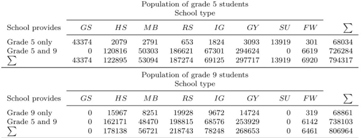
Sampling schools for Starting Cohorts 3 and 4 was done in school year 2009/10 using information on schools from the school year 2008/09. Survey-ing and testSurvey-ing students took place in school year 2010/11. Within these two years fluctuation (students repeating a class or leaving school), ongoing school reforms or closing down of schools reshape the population of schools. In probability proportional to size (pps) sampling (as one measure to achieve an approximate control of sample size) the measure of size is the characteris-tic to which the probability for sampling is proportional to. When choosing
the number of students or the number of classes per school this characteristic might change over time. Using an appropriate measure of size in pps sam-pling on the first stage, that allows for an inverse pps on the second stage results in a sample where each individual has the same design weight, that is, a self weighting sample.1 Since the characteristic for a measure of size inpps
sampling based on information from school year 2008/09 and an inverse pps
based on the same characteristic two years later which might change during that period, an exact self weighting sample can only be realized having a con-stant characteristic. Due to the changes induced by this gap in time different characteristics for constructing the measure of size were evaluated. The aim was to find a measure of size that is stable over this period to get as close as possible to a self weighting sample. The evaluation uses the actual sampling frame from school year 2008/09 and the one from the previous school year 2007/08. The measure of size for sampling was chosen to yield minimum variation of design weights induced by changes due to the gap in time.
Applying the above described stratified two-stage cluster sampling design schools and classes were sampled and corresponding design weights were de-rived for schools and students. The sampled schools (also referred to as orig-inal schools) were contacted by the survey research institute and asked for participation. Since participation is voluntary and schools could refuse each sampled school was assigned up to four replacement schools and if necessary contacted in a fixed order to counteract a reduction of sample size. Within each participating school two classes were sampled if at least three were present, otherwise all classes were sampled. One teacher within each school responsible for communication with the survey research institute (coordina-tor) was asked to list all students in the sampled classes on the so called Schüler-Teilnahme-Liste (engl.: student participation list, see Table B.2). Each student willing to participate had to return an informed consent signed by a parent if the student was not of legal age. This participation status was recorded on the list and it further contained information on the initial sample such as sex, month and year of birth, school type, etc. One part of this list was returned to the survey research institute and later on to the methods department of the NEPS. The other parts remained in the school.
The derived design weights apply to the initial sample of original schools and their students. They would be applicable if participation in the study is mandatory. Since schools as well as students have the possibility to refuse participation the derived design weights need to be adjusted to compensate for refusal (i.e., unit nonresponse). Due to the two-stage sampling design and
1This is true under certain circumstances discussed in more detail in Sections 3.4 and
INTRODUCTION 5
the successive decision processes on each stage unit nonresponse can occur on each stage. Therefore the derived design weights were adjusted on each level, that is, school and student level, successively to correct for unit nonresponse. Adjustments on the school level utilized information from sampling (for ex-ample strata, number of classes, etc.) as well as information arising from the recruitment process of schools (for example number of schools recruited per federal state). Adjustments on the student level utilized information pro-vided by the coordinator on the students participation list. The adjustments of the initial sample were done respecting the structure of the school system, two-stage decision processes and the clustering of students within schools. These adjusted design weights apply to students willing to participate in the panel, that is, the panel cohort, and will be referred to as panel entry weight. At the day of surveying and testing students in schools students were absent due to illness, weather conditions or other reasons although they were willing to participate. The absence of students at ’test days’, referred to as temporary drop-out, can occur in each wave of the panel. This makes further adjustments for wave-specific unit nonresponse necessary. These are based on information available for the entire panel cohort. Adjusted weights for the panel cohort are provided for different groups. These groups include wave-specific participants (cross sectional weights), all-time-participants (panel co-hort members participating in each wave up to the actual wave) or subgroups of interest (for example students and parents or participants with available tests from each second wave).
Wave-specific adjustments correct for unit nonresponse in the correspond-ing wave. Therefore participation decisions are modeled uscorrespond-ing available infor-mation which is mostly not varying over time. To account for the clustering of students a random intercept model is adopted using a probit link function.2
The models will become more sophisticated in the progress of the panel, since more information arises. Information that is missing or not available in the first wave may arise in the second wave so that the model for the first wave can be updated and becomes more accurate.
The group of panel cohort members participating in each wave up to the actual wave, that is, the all-time-participants, is modeled almost analogously to the cross sectional adjustment models. The models are conditioned on the participation status in previous waves and extended by information arising in the progress of the panel.
Finally, models for weighting adjustments in the subgroup of the panel cohort students in grade 5 and their parents have to consider two possibly
2The probit specification is used to be consistent with extensions of the model
correlated decisions. Thereby both, the students and the parental survey are subject to nonresponse. To provide unit nonresponse adjusted weights for the relevant group of participating students and parents, a bivariate probit with random intercept allowing for clustering at the school level is used. Yet there is no implementation of this model for the statistical software package R (R Core Team, 2014) available. Thus it is provided in the Appendix D. The model is estimated using a simulated maximum likelihood procedure based on the importance sampler of Geweke, Hajivassiliou and Keane (GHK-simulator) documented in Geweke and Keane (2001).
The empirical results of the adjustment models point at significance of typical explaining factors of unit nonresponse and reveal the importance to consider a clustering structure as well as a correlation parameter regarding the possibly correlated participation processes of parents and students.
This dissertation proceeds along the order of events. Chapter 2 will give a review on sampling and weighting as basis for the description in the following chapters. Chapter 3 gives detailed insights on the sampling design of SC3 and SC4. The weighting procedures applied to SC3 and SC4 are discussed in Chapter 4. The bivariate probit model with random intercepts and its application to weighting adjustments in SC3 is shown in Chapter 5. A sum-mary and an outlook to future research in the field of weighting longitudinal cohorts with complex survey designs will be given in Chapter 6.
The Appendix A contains the lists of abbreviations and symbols used throughout the following chapters. Appendix B includes the tables in order of their appearance within the text. An illustration of the GHK-simulator is given in Appendix C. The syntax of the code used for estimation of the bivariate probit model with random intercept as introduced in Chapter 5 is displayed in Appendix D. Finally Appendix E gives R’s session information.
Chapter 2
Reviewing sampling and
weighting techniques
Chapter outline:
Reviewing the basic sampling techniques this chapter will serve as theoretical basis for the thorough description of the samples in the subsequent chap-ter. The review deals with the preparation of the sampling frame, a general description of sampling as well as a formal description of deriving design weights. This is followed by a summary of the sampling techniques applied in SC3 and SC4. It finishes with aspects of weighting adjustments.
This chapter is in parts based on the work published in earlier papers by Aßmann et al. (2011) and Aßmann et al. (2012).
2.1
The sampling frame
The starting point for each sampling design is the definition of the target population in terms of temporal and regional restriction as well as further characteristics describing the population. The basis for sampling is most often provided in form of a complete list of population elements1 containing
available information for each element. This complete listing is referred to as sampling frame. Sampling frames usually are obtained from administrative data bases, for example registration offices and their registers or complete lists of schools, universities and communities provided by the States Bureaus of Statistics (Statistische Landesämter).
When requesting administrative listings the frames provided (for exam-ple for schools or communities) cannot always be up to date since ongoing
1The terms element and unit will be used synonymously.
reforms, closing and merging of institutions, deaths and births as well as mi-gration and immimi-gration reshape populations. Therefore any sampling frame available can only be a snapshot of the population at a certain point in time. This in fact has an impact on designing a sampling strategy. Furthermore frames are provided by states in different formats, quality and informational content. So the aim to construct a nationwide frame can become a challeng-ing task. For more details on the provision and harmonization of a frame see Aßmann et al. (2012).
2.2
Sampling techniques
There exist different methods to draw a sample from a target population (also universe) if a sampling frame is available. Let U denote the universe consisting of N units U = {u1, . . . , ui, . . . , uN}. Let further the set of all
samplesS contain all possible sampless of sizenfor a given selection scheme so thats ∈S. The probability p to draw one certain sample s∈S is given by the function p: S →[0; 1] with p(s)> 0 and P
s∈Sp(s) = 1 (see Särndal
et al., 2003, pp. 27f). The tuple (S, p) is called sample design. For a given sample design the first order inclusion probability πi is the probability that
the ith element u
i is sampled (see Särndal et al., 2003, p. 31):
πi =P(ui ∈S) =
X
s3ui
p(s).
The probability that the units ui and uj (i6=j) are sampled jointly into the
sample is given by the second order inclusion probability πij
πij =P({ui;uj} ∈S) =
X
s3{ui;uj}
p(s).
The summation is over all samples s that do contain the element ui. The
design weight di for unit ui is usually given by the inverse of its first order
inclusion probability
di =
1
πi
∀i= 1, . . . , n.
With respect to the design (S, p) for each sampled unit ui the design weight
di can be derived. The design weight (or also base weight) can (in some
designs) be interpreted as the number of population elements represented by a sampled unit (see Wolter, 2007, p. 18). In simple random sampling without replacement the first order inclusion probability arises as
πi =
n
REVIEWING SAMPLING AND WEIGHTING TECHNIQUES 9
Hence the design weight is (see Tillé (2006, p. 45) or Särndal et al. (2003, p. 66)) di = 1 πi = N n ∀i= 1, . . . , n
being constant for all sampled units. In case of simple random sampling without replacement the design weight di gives the number of units
repre-sented in the population by the sampled unit. That is, the sum of the design weights results in the population size N, since
n X i=1 di = n X i=1 n N −1 = n X i=1 N n =n· N n =N.
This is not necessarily the case for all sampling designs. Such is the usual case in sampling with replacement or under consideration of ordering. In statistical inferences constant design weights (as above) can be ignored. In contrast, nonconstant design weights cannot be ignored, since they arise from complex designs such as stratified, multistage or cluster sampling (Snijders & Bosker, 2012). The design weights are commonly used for estimation of population parameters (for example totals, means, ratios) for some variable of interesty. Applying the Horvitz-Thompson estimator (Horvitz & Thompson, 1952) the estimated population total Yb is computed as the sum of weighted
observations of yi for unit ui ∈s
b YHT = n X i=1 yidi = n X i=1 yi πi .
For a probability distribution p on S and a general estimator τ the tuple (p, τ) is referred to as strategy. One main focus of sample selection theory therefore is to find sample designs well interacting with estimators, which means finding appropriate strategies. To achieve this aim it is necessary in advance to be aware of analyses of interest when the sample is realized and information is available.
But designing a sampling scheme also has to take practical and econom-ical aspects into account. Complex survey designs often do not allow for sampling units by simple random sampling. Economic reasons finally drive decisions towards certain sampling designs, even if those result in more com-plex methods of data analysis. The aim of providing accurate estimates for a population of interest is often achieved by choosing other designs than simple random sampling.
2.2.1
Explicit Stratification
Explicit stratification assigns each population element ui to distinct
non-overlapping strata. After stratifying the populationU inh= 1, . . . , H strata
U1, . . . , UH with population sizes N =PHh=1Nh samples of size nh are taken
independently from each stratum. Explicit stratification serves several aspects as discussed in Kish (1995, pp. 76-77) and Särndal et al. (2003, p. 100).
• It can be used to gain precision in estimates (i.e. decrease their vari-ance).
• By sampling independently from each stratum different sampling de-signs can be applied to the strata. This is especially useful when the populations are extremely heterogeneous or their elements differ by nature.2
• Stratification by cluster size is one possibility to control sample size in case of clusters with unequal size.3
• When samples are drawn from several frames of different quality strat-ification may become necessary. Characteristics that are relevant for sampling may be measured differently, provided in a different way or even be missing.4
• Subpopulations can be of special interest for a study and separate esti-mates are needed. Dividing the population in strata serves this aspect.5
• Administrative reasons may be a further argument for stratification.
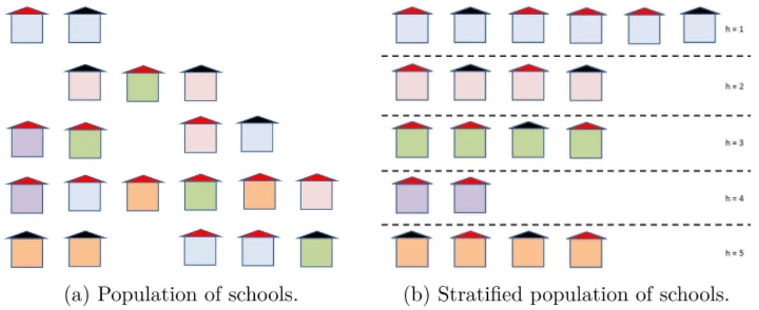
Figure 2.1 illustrates explicit stratification of schools. The schools in the population (Subfigure 2.1a) are assigned to the stratah= 1, . . . ,5. Thereby each stratum can contain a different number of schools. The schools within each stratum are in this example identical with respect to the stratification characteristic color of the school building6 (Subfigure 2.1b) but still different
with respect to other characteristics (for example color of the roof). When
2This aspect applies in sampling students. The samples were stratified by school type
to account for heterogeneity between different school types; especially between regular and special schools.
3See also Section 2.2.2 for further details.
4This issue is addressed in Section 3.4 and 3.5 for sampling students in regular (
allge-meinbildende Schulen) and special (Förderschulen) schools.
5This is shown in Section 3.4 when oversamplings of students in vocational tracks are
considered.
REVIEWING SAMPLING AND WEIGHTING TECHNIQUES 11
(a) Population of schools. (b) Stratified population of schools.
Figure 2.1: Explicit stratification of schools by color of the school building.
using explicit stratification sample size (for example n = 10) needs to be allocated to the strata. The allocation of the total sample size n to the H
strata can be achieved in several ways whereas it always has to be ensured that n = PH
h=1nh (Cochran, 1977, p. 89). In equal allocation sample size
per stratum nh = Hn is equal across strata n1 =n2 =. . .=nH (for example
sample nh = 2 blue, red, green, purple and orange schools). Allocating
the total sample size proportional to the size of the population of stratum h
results in unequal sample sizes per stratumnh =n·NNh (for example 3 blue, 2
red, 2 green, 1 purple and 2 orange schools) and equal sampling fractionsf =
nh
Nh. To gain precision in estimates for small strata the sample size is increased
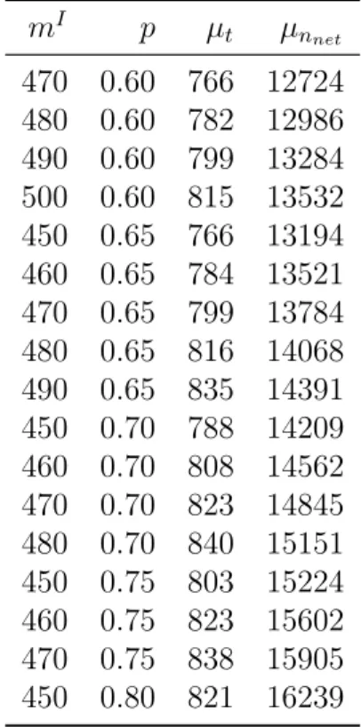
resulting in unequal sampling fractions. This is called oversampling of strata. To ensure a minimum (and maximum) number of sampling units per stratum Gabler, Ganninger, and Münnich (2012) derived an allocation algorithm with respect to bounded design weights while considering optimality in allocation for stratified random sampling.7 For a numerical solution see Münnich, Sachs,
and Wagner (2012)
Explicit stratification results in independent samples. If this is not de-sired or possible implicit stratification, that is, sorting the sampling frame by characteristics available, together with systematic selection can–to some extend–help to ensure having elements of implicit strata within the sample. The result will be similar to that of a proportionate stratified sample (Kish, 1995, p. 85). Implicit stratification will not be useful for small strata (for example purple schools in Subfigure 2.1b), since they may not be sampled or only in small numbers.
7This approach was discussed in sampling the Starting Cohort 1 – Early Childhood of
Besides explicit and implicit stratification it is also possible to stratify the sample after its realization. When information is not available for sam-pling but is collected during the field period (for example individual char-acteristics such as age, sex, occupation) these information can be used for post-stratification.
2.2.2
Multistage and multistage cluster sampling
Multistage sampling is used to get access to hierarchical structured or clus-tered populations. Sometimes it is not possible to sample individuals directly, since no frame is available on the individual level. In this case clusters of individuals can be sampled instead if the individuals are grouped or clus-tered (and there is an available frame). In cluster sampling a cluster (for example a school) contains a set of units (students) and within a cluster all units can be surveyed (Särndal et al., 2003, p. 124). If further samples are drawn within the cluster, sampling is done on multiple stages and is therefore referred to as multistage sampling. In two-stage sampling units on the first stage are referred to asprimary sampling units(PSU, e.g. schools) and those on the second stage are called secondary sampling units (SSU, e.g. classes). The primary sampling units on the first stage are disjoint sub-populations of grouped secondary sampling units. In multistage designs this hierarchy is extended to the ultimate stage (Särndal et al., 2003, p. 125) and sam-pling selection processes can differ at each stage so that the variety of designs increases rapidly.
Except for the case of equal sized clusters on each stage the resulting sample size becomes a random variable and is not under control (see Kish, 1995, pp. 217ff or Särndal et al., 2003, p. 127). Controlling sample size is essential to most surveys because there are variable costs increasing the total costs by each sampled unit. Kish (1995, p. 217) points out that "Exact control of sample size is unnecessary and impossible in most situations. [...] We should aim at anapproximate control that is both feasible and desirable." To achieve this approximate control in the case of unequal cluster size Kish recommends not to use uncontrolled random sampling procedures and to stratify by cluster size. Another way is to split or combine clusters of unequal size to clusters of a more similar size. On the second stage also size stratified sampling can be applied with different sampling fractions or a fix number of elements can be sampled. Finally probability proportional to size sampling of units (no matter on which stage) can help to get less variation in the initial sample size (Kish, 1995, pp. 219f). In probability proportional to size sampling each sampling unit is assigned a measure of size (mos) which can be a natural characteristic of that unit (for example number of students
REVIEWING SAMPLING AND WEIGHTING TECHNIQUES 13
of a school) or any value assigned to it (Kauermann & Küchenhoff, 2011, pp. 104f).
Mehrotra, Srivastava, and Tyagi (1987) show another way for controlling sample size by discarding an excess number of clusters randomly from the sampled clusters. The advantages of the proposed procedure are convergence of planned and realized sample sizes and thereby a reduction of survey costs. But discarding clusters from the sampled clusters therefore results in less effi-cient estimators. Discarding clusters can be done if information about cluster size is reliable or can be estimated accurately. When sampling and survey-ing is done at different points in time cluster size can change significantly and though discarding clusters can become a challenging task.8 Furthermore
Aliaga and Ren (2006) determine the optimal number of clusters to sample in a two-stage design for a given linear cost function.
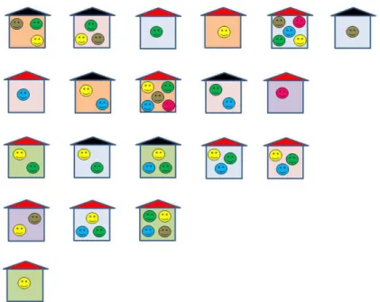
Figure 2.2: Two-stage cluster sampling.
Figure 2.2 illustrates clusters of students (i.e., classes) in schools. The classes indicated by colored smileys are located within schools. In two-stage cluster sampling a number mI of primary sampling units CI (e.g. schools)
is sampled on the first stage (denoted by the superscript). Within a
sam-8In NEPS sampling schools was based on a frame of the school year 2008/09. Sampling
was done in 2009 and surveying and testing of students followed in school year 2010/11. See Section 3.4 for further details.
pled first stage cluster CI
j a number mII of secondary sampling units CII
(e.g. classes, colored smileys) is sampled. To demonstrate the problem of unequal cluster sizes let the yellow smileys be classes of 20 students, the green smileys be classes of size 25 and the brown smileys classes of size 30. Having sampled two schools (e.g. the first and the second in the top row) and sampling one class per school the sample sizes can vary. Sampling a yellow and brown smiley will result in the same sample size as sampling two green smileys. But any other combination will either yield smaller sample sizes (green and yellow, yellow and yellow) or larger sample sizes (green and brown, brown and brown). So, depending on the samples drawn, the sample sizes can be n∈ {40; 45; 50; 55; 60}.
2.2.3
Systematic and systematic unequal probability
sampling
Systematic sampling is an alternative to random selection of units. In sys-tematic sampling with equal probabilities each unit is assigned an interval of length 1 (for illustration see Figure 2.3). The selection interval length
k = Nn is the population size N divided by the sample size n. Starting from a randomly drawn starting pointr∈ {1, . . . , k}(i.e. within the first interval) every kth unit is selected. The units u
i selected by systematic sampling are
then
s={ur, ur+k, ur+2k, , ur+3k, . . . , , ur+(n−1)k}
and the inclusion probability for each unit i is the same πi = 1k (Madow,
1949). The only unit sampled randomly is the first one. Since the rest of the sample is determined by the first unit sampled. Systematic selection can be seen as single stage cluster sampling where only one cluster is selected (Kauermann & Küchenhoff, 2011, p. 172).
One drawback of systematic selection is that some units ui and uj do
not have a second order inclusion probability πij. For example let ui and
uj be neighbours, than there is no chance for them to end up together in
a sample. This drawback mainly effects variance estimation, for example for the Horvitz-Thompson estimator. An overview of variance estimation methods that can be applied in this and other cases is given in Münnich (2008). A more details can be found in Wolter (2007).
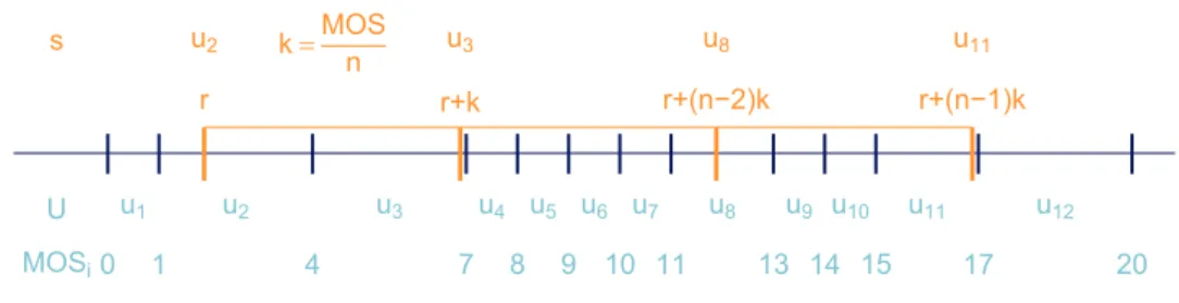
Figure 2.3 illustrates sampling n = 12 units from a population of size
N = 120 via systematic sampling with a random start value 0 < r ≤ 12. TheN units of the population are ordered on the axis, where each tick mark indicates one unit. The interval length between to neighbouring units is
REVIEWING SAMPLING AND WEIGHTING TECHNIQUES 15
1r N
k
Figure 2.3: Systematic selection of units with random start.
equal to 1. Let r = 3 and k = 12012 = 10 then the sample would consist of the units s={u3, u13, . . . , u113} (indicated by the larger tick marks and the
arrows). This selection procedure is easily applicable but also can become more sophisticated for example when it comes to selection with probability proportional to size or whenkis not an even number. For a brief discussion of systematic sampling procedures see Madow and Madow (1944) and Madow (1949, 1953). For extension to circular methods as solution to non-integer k
see Uthayakumaran (1998) or Kish (1995, p. 116)
In systematic sampling (as well as other random sampling procedures) units can be sampled with unequal selection probabilities. When systematic sampling is performed with pps each unit ui is assigned a measure of size
mosi. The total measure of size is
M OS = N X i=1 mosi and M OSi = i X j=1 mosj
is the cumulative measure of size and the selection interval lengthk changes tok = M OSn (see Kish (1995, pp. 234ff) or Hájek and Dupač (1981, p. 113)). The inclusion probability for unitithen arises asπi = nM OS·mosi, see Tillé (1996)
or Wolter (2007, pp. 332ff).
Table 2.1: Example for systematic probability proportional to size sampling.
u1 u2 u3 u4 u5 u6 u7 u8 u9 u10 u11 u12
mosi 1 3 3 1 1 1 1 2 1 1 2 3
M OSi 1 4 7 8 9 10 11 13 14 15 17 20
Note: Systematicppssampling is performed usingppss()implemented in the packagepps(Gambino, 2012). Use this function with care, since it can not handleπi>1.
Table 2.1 shows a simple example for a universe consisting of 12 units. From this universe a sample of sizen = 4 is taken using systematic probabil-ity proportional to size sampling. With random start point r = 1.8812 and
interval lengthk = 5 the unitsu2, u3, u8 and u11 are sampled. Using
system-atic unequal probability sampling two neighbouring units can be selected, see Figure 2.4.
| |
|
| | | | |
| | |
|
|
MOSi0 1 4 7 8 9 10 11 13 14 15 17 20 U u1 u2 u3 u4 u5 u6 u7 u8 u9 u10 u11 u12|
|
|
|
u2 u3 u8 u11 s k=MOS n r r+k r+(n−2)k r+(n−1)kFigure 2.4: Graphical illustration for pps sampling according to Kish (1995, pp. 230, 234ff).
Figure 2.4 gives the graphical illustration of the example above. The cumulative measure of size M OSi is given along the axis. The first unit
selected is the unit which includes the random start r in its interval. From this starting point each element is chosen, whose interval includes r plus a multiple ofk.
2.3
Design weights and their adjustment
Since non-mandatory surveys are typically affected by nonresponse. Nonre-sponse may occur for several reasons. Lepkowski and Couper (2002) separate the process leading to participation or nonparticipation into location of units, contacting units (given location) and cooperation of units (given location and contact). Therefore sampled units can end up as nonrespondents in each of the three steps. For example a sampled unit has moved and thus cannot be located. Other units might–for whatever reason–not be contactable. For example they can be in a hospital because of illness or have moved abroad. Thus these persons can not be contacted and asked for participation. Some of the sampled, located and contacted units will refuse to participate in the survey. Reasons for refusal vary between countries, survey topics, etc., see for example Lugtig (21.10.2013) These groups of people, that is those people that could not be located, contacted and those that refuse to participate, form the set of nonrespondents. This so called unit nonresponse might make adjustments of the design weights necessary, depending on the type of the
REVIEWING SAMPLING AND WEIGHTING TECHNIQUES 17
missing data mechanism. The derivation of final weights is, according to Kalton and Kasprzyk (1986), in general done in three steps:
1. Derivation of design weights
2. Sample weighting adjustments
3. Population weighting adjustments
In the first step design weights (also known as base weights) are usually computed as the inverse of the inclusion probability (as shown in Section 2.2). Thus, for most designs they are directly available after sampling. De-sign weights compensate for unequal probabilities of selection, unequal sam-pling fractions in stratified samples, that is, oversamsam-pling, or for subsamsam-pling (Kish, 1990, 1992).
In the second stepthe design weights are adjusted to correct for unit non-response. Kalton and Kasprzyk (1986) refer to this step as sample weighting adjustment. In multistage sampling procedures this step needs to be con-sidered on each stage where nonresponse occurs. Sample weighting adjust-ments correcting for unit nonresponse usually result in increasingly varying weights and thereby lower the precision of survey estimates (Kalton & Flores-Cervantes, 2003).
The third step, referred to aspopulation weighting adjustment, calibrates weights so that estimates conform to known parameters (for example totals or ratios) of the population. This last step corrects for potential bias due to incomplete coverage or non-coverage of the population and sampling error (Brick, 2013).
2.3.1
Sample weighting adjustment
After the sample is realized the sampled units have to be contacted and are asked to participate in the survey. This two stage process gives rise to two rea-sons why sampled perrea-sons might not be surveyed. Survey response depends on contact and cooperation. First, the sampled unit needs to be contacted. Second, given contact the unit decides to cooperate or not. Failing to estab-lish contact as well as noncooperation will result in unit nonresponse, but for different reasons (Groves, 1998). Survey response therefore can become a threefold variable of participation, refusal and noncontact.When modeling unit nonresponse the two components, that is noncontact and refusal, should be modeled to avoid bias (Steele & Durrant, 2011). For both components of unit nonresponse the resulting sample will be biased if the persons not participating form a selective group.
The need for adjustments of the design weights depends on the missing data mechanism. The terminology originates from item nonresponse and multiple imputation, see Rubin (1987) or Little and Rubin (2002). But it is also applicable in the context of weighting adjustments. Therefore we need to come back to the strategy. The aim of every survey is to investigate on a variable of interest (y, for example educational aspirations) and use auxiliary information (x, for example educational degree of parents). Unit nonresponse causes both variables to be missing.
A unit is said to be missing completely at random (MCAR) if the prob-ability of responding is depending neither on observed nor on unobserved characteristics. An extreme MCAR case would be if any person in the sam-ple has the same response probability (Valliant, Dever, & Kreuter, 2013). In this case the responding part of the sample is a random subsample of the entire sample that allows for valid inferences. An example would be a student being ill at the day of the survey or a computer crash in computer based assessments.
Unit nonresponse is missing at random (MAR) if the probability of re-sponse depends on the data but only the auxiliary information available for respondents and nonrespondents. This information can either be marginal distributions from a census or individual-level data available for the entire sample. If this auxiliary information is at hand, a model for response propen-sities can be estimated. Lohr (2010) describes this asignorable nonresponse. That is if a model can explain the mechanism of nonresponse and that it can be ignored if it is accounted for. This approach does not only allow for re-weighting the initial sample but also for documenting effects significantly influencing participation decisions. Therefore it is used in later re-weighting. Here it is not that nonresponse can be ignored and complete data methods can be applied. In the example MAR would be if the probability of response would depend on the educational degree of the parents which is observed.
When the probability of nonresponse depends on the variable of interest (y, for example educational aspirations) and cannot be accounted for by modeling the response based an the auxiliary information (x) units are not missing at random (NMAR). (Valliant et al., 2013, p. 319) also term this nonignorable nonresponse. This type of missing data mechanism is–if at all– hard to detect. One way of finding out about NMAR would make follow-ups necessary.
To correct for potential bias arising through unit nonresponse there are a variety of procedures available. Weighting is one of the most commonly used methods to correct for unit nonresponse in surveys (Little & Vartivarian, 2003). A general overview on weighting methods to correct for unit nonre-sponse is given by Kalton and Flores-Cervantes (2003). A more technical
REVIEWING SAMPLING AND WEIGHTING TECHNIQUES 19
overview is given by Holt and Elliot (1991).
One way is to adjust the number of participants to the initial sample size. That is the weight is multiplied by an adjustment factor δ
wi =di·δ, with δ=
nr+nn
nr
. (2.1)
Here nr denotes the number of participants and nn the number of
nonpar-ticipants. This approach implicitly assumes that unit nonresponse occurs completely at random. It can be extended in two directions. First the ad-justment factor can be derived as the fraction of the sum of weights for all units divided by the sum of weights for the respondents. This is more appropriate in probability proportional to size samples. Second the above approach and the first extension can be modified by adjusting the weights within certain cells. These cells are formed by characteristics of the units themselves or of higher level units. For example the cells can be defined by sex, age group and cluster. This approach is referred to as cell weighting and is one of the most commonly used approaches to correct for unit nonresponse in (sample) weighting adjustments (Rässler & Riphahn, 2006; Rässler & Schnell, 2003).
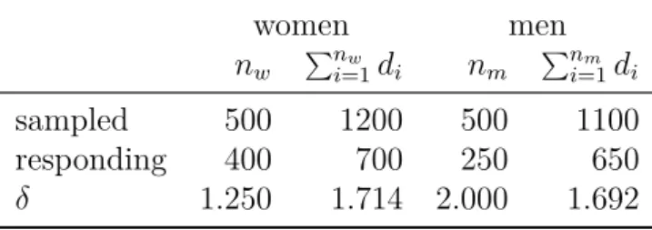
Table 2.2: Example for cell weighting.
women men
nw Pni=1w di nm Pni=1m di
sampled 500 1200 500 1100
responding 400 700 250 650
δ 1.250 1.714 2.000 1.692
Assume the realization of a sample of size n= 1000 (shown in Table 2.2) with an equal ratio of women and men (i.e.nw =nm, of course just for
conve-nience), whereasnw = 400 women and nm = 250 men respond to the survey.
A naive approach would be adjusting the design weights neglecting infor-mation on sex resulting in an adjustment factor δ = 1000650 ≈ 1.538. Making use of the information on sex results in gender specific participation rates of
pw = 400500 = 0.8 andpm = 250500 = 0.5 and the corresponding adjustment factors
(see Equation (2.1)) δw =p−w1 = 500 400 = 1.25 and δm =p −1 m = 500 250 = 2.0.
Bas-ing the adjustments on the sum of weights would lead to adjustment factors for women δw = 1200700 ≈1.714 and menδm = 1100650 ≈1.692.
A more sophisticated approach is to adjust the respondents by the in-verse of their estimated response propensity. The basic idea (harking back
to Rosenbaum and Rubin (1983)) is to find a sampled element that is most similar to the refusing. Now this similar element has to "represent" more pop-ulation elements. To do so the response propensity is most often estimated using logit9 models for binary data, which need information on participants
as well as non-participants. The inverse of the estimated response propensity
b
λi for element i is multiplied by the design weight and finally the adjusted
design weight is (Rendtel & Harms, 2009)
wi =di·λb−1
i . (2.2)
Frameworks that can be applied to estimate these response propensities are more thoroughly discussed in Section 4.2. Note that di is a fixed value
de-pending on the sample design (S, p) only. The value ofwi, since multiplied by
b
λ−i 1 estimated from a model, in contrast is an estimate based on the realized sample. Asymptotic properties of estimators using nonresponse adjusted de-sign weights wi based on the estimated response propensity are discussed by
Holt and Elliot (1991), Kim and Kim (2007) and Henry and Valliant (2012).
2.3.2
Population weighting adjustment
The idea behind population weighting adjustments is to make sample dis-tributions and parameters conform to known disdis-tributions and parameters of the population. For population weighting adjustment most of the meth-ods used in sample weighting adjustment can be applied as well (Kalton & Flores-Cervantes, 2003). Unlike sample weighting adjustments population weighting adjustments do not need information for nonrespondents (Brick & Kalton, 1996). For population weighting adjustments distributions or pa-rameters of the population need to be known. Further methods for popula-tion weighting adjustments include calibrapopula-tion, general regression estimapopula-tion (GREG), raking or post stratification.
Post stratification can make use of data collected in the survey that was not available before (for example age or sex). For known totals of subgroups of the population the weights for units are adjusted within subgroups (or classes, poststrata) so that the estimate conforms to the total within this class. This method therefore reduces bias induced by undercoverage. One problem with this approach arises if the characteristics used in forming the poststrata are not measured in the same way for the sample and the popula-tion (for example migrapopula-tional background). Never the less post stratificapopula-tion
9Laaksonen (2005) finds the logit link function to be used most often and further
discusses the characteristics of probit, log-log and clog-log. In his findings the choice of link functions only differs slightly in estimated propensities.
REVIEWING SAMPLING AND WEIGHTING TECHNIQUES 21
is, according to Brick and Kalton (1996), one of the most frequently used population weighting adjustments.
For a large number of characteristics available for the sample and the population together with parameters of interest post stratification may suffer from small number of cases within the poststrata. In this case an iterative approach called raking is superior. It iteratively adjusts the weights in a way that marginal distributions of auxiliary information conform to those of the data (Brick & Kalton, 1996). The approach, also referred to as iterative proportional fitting, was suggested by Deming and Stephan (1940)
The calibration approach systematically incorporates auxiliary informa-tion into the procedure (Särndal, 2007). Calibrainforma-tion thereby is not only a procedure for population weighting adjustment, but also incorporates the estimation of population parameters. The weighting adjustment computes weights using auxiliary information. These adjustments are–at the same time–restrained to one or more calibration equations, see Särndal (2007).
General regression estimation is another way to incorporate auxiliary in-formation in the estimation step. Deville and Särndal (1992) note that the GREG can be derived also from calibration by focusing on the weights. They show that the weights used in GREG are closely to those derived by calibra-tion according to a given distance measure. A disadvantage of using GREG is that negative weights can occur (Deville & Särndal, 1992).
In the later application we refrain from population weighting adjustments, since there are either no known population parameters (yet) available to adjust to or these are based on non-matching definitions.
Chapter 3
Sampling grade 5 and grade 9
students
Chapter outline:
The samples for students in grade 5 and 9 in secondary schools (Starting Cohorts 3 and 4) will be thoroughly described in this chapter. The populations of students in grade 5 and 9 are described using available information from the sampling frame. On the basis of this information the planning phase with simulations and their corresponding results are presented. The final description of the samples for grade 5 and grade 9 students is then associated by the derivation of design weights. The sampling design of NEPS can be summarized as a stratified multistage cluster sampling design. The selection scheme, that is, the rule of how to select units from the universe, for sampling PSUs is systematic selection with probability proportional to size and the SSUs are sampled using simple random sampling. The focus therefore will be on the particularities of each Starting Cohort.
This chapter is in parts based on the work published in earlier papers by Aßmann et al. (2011) and Aßmann et al. (2012).
3.1
Population
The target population of the NEPS SC3 and SC4 include all students attend-ing primary or secondary schools in grade 5 or grade 9 within the Federal Republic of Germany in the school year 2010/11. Access to the popula-tion of students was gained via the corresponding set of schools. This set of schools includes all officially recognized and state-approved educational institutions within the Federal Republic of Germany providing schooling for students in grade 5 and / or grade 9. Excluded from the population were
students attending vocational schools or schools with a predominant foreign teaching language that would hinder the realization of a complete survey procedure with the test instruments available. Further, students attending regular schools being unable to follow normal testing procedures were ex-cluded.1 Additionally, the NEPS comprises a sample of students attending special schools with main emphasis on special educational needs in the area of learning. Access to this population was gained via special schools with Federal-State-specific provisions explicitly for students with special educa-tional needs in the area of learning. Overall, 80% of students attending special schools have a diagnosed learning disability – constituting the largest group of students in these schools. For more details see also Aßmann et al. (2011).
Table 3.1 shows the population of regular schools by school type and schools having classes in grade 5 and 9. The population of schools consists in total of 29346 schools from which 16273 are of no interest for sampling students in grade 5 or 9 since they neither have any classes in grade 5 nor any in grade 9 (row: Neither grade). Although these schools can have classes in any other grade from 1 to 4 and from 6 to 8. The middle rows give the number of schools having only classes in grade 5 and none in grade 9 (row: Grade 5 only) and vice versa. That is the number of schools having classes only in grade 9 but none in grade 5 (row: Grade 9 only). Schools having only classes in grade 5 are in total 1459 and schools having only classes in grade 9 are 1281. The majority of schools relevant for sampling students in SC3 and SC4 consists of secondary schools having classes in grade 5 and grade 9 are in total 10333 (row: Grade 5 and 9).
Table 3.1: Population of regular schools by school type and schools providing classes in grades 5 and 9 (school year 2008/09).
School type GS HS M B RS IG GY SU F W P Neither Grade 16109 17 72 14 4 44 4 9 16273 Grade 5 only 913 89 75 25 58 62 222 15 1459 Grade 9 only 0 447 163 346 84 230 0 11 1281 Grade 5 and 9 0 3656 1044 2211 541 2708 0 173 10333 P 17022 4209 1354 2596 687 3044 226 208 29346
Notes: Abbreviations of school types areGS: Grundschule,HS: Hauptschule,M B: Schule mit mehreren Bildungsgän-gen,RSRealschule, IG: Integrierte Gesamtschule,GY: Gymnasium, SU: Schulartunabhängige Orientierungsstufe and F W: Freie Waldorfschule.
1Regular schools are allallgemeinbildende Schulen according to the definition of
SAMPLING GRADE 5 AND GRADE 9 STUDENTS 25
Later on the school types Integrierte Gesamtschule (IG) and Freie Wal-dorfschule (F W) will be joined in one stratum since the degrees achievable are similar. Further school typesGrundschule(GS) andSchulartunabhängige Orientierungsstufe (SU) will be joined in one stratum because these schools educate students in grade 5. The school typeGSsummarizes primary schools normally educating students in grade 1 to 4. The 913 schools having grade 5 too are schools in Berlin and Brandenburg educating students from grade 1 to grade 6. School typeSU educates students only in grade 5 and 6 in Hesse and Hamburg.
For the population of schools displayed in Table 3.1 the number of stu-dents within these schools are given in Table 3.2. The table is twofold since the number of students in grade 5 and 9 needs to be reported separately.That is because grade 5 students can be in schools providing either classes in grade 5 only or they can be in schools providing classes in grade 5 and 9. For example there are 2708 Gymnasia (GY) providing access to students in grade 5 and students in grade 9. These 2708 schools educate 294624 students in grade 5 (Table 3.2 upper half) and 253929 (Table 3.2 lower half) students in grade 9. Further there are 62 Gymnasia providing access to 3093 students in grade 5 only and 230 Gymnasia educating 14724 in grade 9 only.2 In total
there are 794317 students in schools providing at least one class in grade 5. The corresponding number of students in schools providing at least one class in grade 9 is 806964.
The zeros in the table are due to the fact that the group of schools pro-viding access to classes in grade 5 and 9 do not have students in grade 5 for school types GS and SU (upper half of the table). These school types educate students only in grades from one to four (GS) and five and six (SU) respectively. So there are no classes in grade 9. In the lower half of the table the zeros arise from school types GS and SU not providing any classes in grade 9.
3.2
Summarizing sampling for school cohorts
The variety of Federal-State-specific school systems is challenging for sam-pling grade 5 and grade 9 students. Several school types related to differ-ent transitions between elemdiffer-entary and secondary school institutions form
2Suppose a Gymnasium has one class in grade 5 having 17 students and one class in
grade 9 having 33 students. This school is reported together with the 2708 Gymnasia having classes in grade 5 as well as in grade 9 in Table 3.1. In Table 3.2 the 17 students in grade 5 are reported among the 294624 fifth grade students and the 33 ninth grade students are reported among the 253929 students in grade 9.
Table 3.2: Population of Students in grade 5 and 9 by school type and schools providing classes in grades 5 and 9 (school year 2008/09).
Population of grade 5 students School type
School provides GS HS M B RS IG GY SU F W P
Grade 5 only 43374 2079 2791 653 1824 3093 13919 301 68034
Grade 5 and 9 0 120816 50303 186621 67301 294624 0 6619 726284
P 43374 122895 53094 187274 69125 297717 13919 6920 794317
Population of grade 9 students School type School provides GS HS M B RS IG GY SU F W P Grade 9 only 0 15967 8251 19928 9672 14724 0 319 68861 Grade 5 and 9 0 162171 48470 198815 68576 253929 0 6142 738103 P 0 178138 56721 218743 78248 268653 0 6461 806964
Notes: Abbreviations of school types areGS: Grundschule,HS: Hauptschule,M B: Schule mit mehreren Bildungsgän-gen,RSRealschule, IG: Integrierte Gesamtschule,GY: Gymnasium, SU: Schulartunabhängige Orientierungsstufe and F W: Freie Waldorfschule.
the set of schools providing access to the target population of grade 5 and grade 9 students. To reflect this variety, seven explicit strata have been de-fined to sample schools. The first stratum comprises all Gymnasien (stratum
GY: Gymnasien), the second stratum consists of all Hauptschulen (stratum
HS: Hauptschulen), the third stratum refers to all Realschulen (stratum
RS: Realschulen), the fourth to comprehensive schools (stratum IG: Inte-grierte Gesamtschulen, Freie Waldorfschulen), the fifth includes schools with several courses of education (stratum M B: Schulen mit mehreren Bildungs-gängen). The sixth explicit stratum comprises schools offering schooling to students with special educational needs in the area of learning (stratumF S: Förderschule). The seventh explicit stratum comprises all schools providing schooling to grade 5 students, but not to grade 9 students (stratum N5). The definition of these seven explicit strata allows fulfilling two important aspects.
1. A requisite of NEPS is to establish a sample of grade 9 students as the starting point of a longitudinal survey of young adults entering voca-tional education over the coming years. In order to ensure sufficient sample sizes for statistical analyses within this heterogeneous popula-tion, who, to a large extent, come from Hauptschulen, Gesamtschulen, and Schulen mit mehreren Bildungsgängen, NEPS comprises an over-sampling of grade 9 students attending these school types.
2. Most secondary schools offer schooling to grade 5 and grade 9 students, so that they can be reached via the same set of schools and, thus,
SAMPLING GRADE 5 AND GRADE 9 STUDENTS 27
reducing administrative survey costs.
In addition to the explicit stratification according to school types, an implicit stratification, that is, sorting the frame by certain characteristics, based on Federal States, regional classification, and sponsorship was used. Given the first-stage sample of regular schools, on the second stage two school classes within each school were sampled randomly, if at least three classes were present, otherwise all classes were surveyed. In special schools a census for all students was held.
3.3
Planning samples for school cohorts
3.3.1
Sample design
For sampling of students in Germany a sampling frame containing a com-plete listing of all students is not available. In contrast a comcom-plete listing of schools providing access to students is available through the Statistical Offices. Access to the target population is gained via the corresponding in-stitution, so that cluster sampling is appropriate. Furthermore the entire age group or only a part of it can be surveyed. When subsampling of age group within a school is performed this is referred to as two-stage (in more general multistage) sampling. One more aspect to consider is stratification since the landscape of school systems in Germany is heterogenous. The population of schools and students was stratified by the school type–more precisely the degree a student can achieve at the school. Lastly there are several selection schemes (i.e., the rules of how to select units from the universe) for sampling units in stratified or multistage designs including simple random sampling (with or without replacement), systematic selection and unequal probability designs. Because the context of the learning environment, that is classes, should be reflected in the data later on cluster sampling of a certain num-ber classes was applied in regular schools. In special schools a census was preferred.
3.3.2
Determining the measure of size
As discussed in Subsection 2.2.2 sampling clusters of unequal size, for exam-ple schools or classes, leads to a random samexam-ple size on the level of students. One way of achieving an approximate control of sample size on the student level is probability proportional to size sampling. Forppssampling a measure of size is assigned to each unit. Using such a sampling design larger schools can be preferred over smaller by assigning them a larger measure of size.
This allows for reducing survey costs by sampling fewer schools to achieve an equal sample size compared to simple random sampling. On the school level characteristics