Wage Mobility Through Job Mobility

WAGE MOBIITY THROUGH JOB MOBILITY

∗∗∗∗

Marcela C. Perticara

+

Universidad Alberto Hurtado

Abstract

The purpose of this paper is to study the relationship between job mobility and wage mobility. One of the main points of this paper is that job mobility is not necessarily bad. Job mobility might be the quickest way in which workers can advance in their careers and move up in the wage structure. Specifically I am going to distinguish between voluntary and involuntary job changes in both the modeling of job mobility behavior and the determination of the wage gains associated with job changing activities.

Using the National Longitudinal Survey of Youth data, I find that workers voluntarily leave their jobs whenever they find themselves being paid below the customary wage rate. In particular, a worker that earns 30% less than the average wage for a worker with his characteristics and labor market experience is more than one and a half times as likely to initiate a separation than a worker just earning the average wage rate. Conversely, a worker earning 30% more than the average wage for a worker with his qualifications and labor market experience faces almost a 50% higher risk of being laid-off. I also show that the informational content on this wage difference seems to decline as the worker acquires more experience (and presumably he learns more about his true productivity) or as the employer information sources increase. All these results are consistent across models.

Workers’ post-separation wage gains also depend on this distinction. Voluntary job changes lead, on average, to gains on the order of 7%, while layoffs imply losses of 5%. That is, voluntary separations, on average, allow workers to improve their relative position in the wage structure. Laid-off workers, however, tend to perform poorly after experiencing a separation. Fifty-percent of the laid-off workers experience wage losses, while 70% of the voluntary job changes end in wage gains. Although quitters have positive wage gains on average, a fairly high amount of quits end up with wage losses. Quitting seems to be a risky, but very rewarding activity. Moreover, while at early stages of the career, workers experience large wage gains from quitting, these gains seem to disappear as their careers extends. Laid-off losses increase as the career extends, particularly for high-skilled workers.

∗ _{This paper is based on two chapters of my dissertation. A reduced version is currently under review for} submission. Thanks to my advisor Dr. Finis Welch and committee members Dr. Donald Deere and Dr. Manuelita Ureta for advice and comments. Bill Gould, Roberto Gutierrez, Vince Wiggins, and others also provided helpful comments during the December 14th 2001 seminar at STATA Corporation. I also thank Alejandra Mizala, Rodrigo Cerda and others for very enlightening comments during the October 23rd 2002 CEA seminar and during the September 2003 PUC seminar.

+ _{Contact information: Marcela Perticara, Erasmo Escala 1835, Room 207. Ph: (56-2) 692-0267. Fax: (56-2)} 692-0303. Email: [email protected].

1.

INTRODUCTION

Job mobility is one of the outstanding characteristics of the US labor market. Few workers stay with the same employer throughout their working lives. There is a large body of literature that theoretically and empirically examines the relationship between long-term wage gains and job mobility. Several papers have also analyzed the changes in job stability and security in the US in past decades as well as their effects on wage mobility. In most of this literature, job mobility is often associated with job instability

(Bernhardt et al., 1999; Monks and Pizer, 1998)

. The main argument in this literature is that, while having many employers may not necessarily be a bad thing, chronic long-term job instability is detrimental to worker’s human capital accumulation and wage growth.

This paper studies the relationship between job mobility and wage mobility. One of the main results is that job mobility is not necessarily bad. Job mobility might be the quickest way in which workers can advance in their careers and move up in the wage structure. Specifically I distinguish between voluntary and involuntary job changes in both the modeling of job mobility behavior and the determination of the wage gains associated with job changing activities. The distinction proves to be relevant.

In the empirical studies on the impact of job mobility on wages most papers have focused on wage changes during transitions. Examples include Keith and McWilliams

(1997; 1999)

, Bartel and Borjas

(1981)

, Mincer

(1986)

, Topel and Ward

(1992)

, Loprest

(1992)

, and Antel

(1983; 1986)

. The common finding is that job mobility leads to wage gains (in levels) during transitions. These studies find mobility gains that range between 10% and 20%. With the exception of Antel

(1983;

1986)

, Moore et al.

(1998)

and McLaughlin

(1991)

, few empirical papers distinguish between voluntary and involuntary separations at the time of calculating average mobility returns or at the time of modeling job mobility.

Using the National Longitudinal Survey of Youth data, I model the hazard of experiencing a job separation primarily as a function of the wage premium the worker is receiving over the wage he would expect to get if he chose to leave his current employer. The expected wage rate is approximated as a function of labor market characteristics and education. Separate estimations for the hazard of voluntary separations and layoffs reveal that both processes indeed look different. I find that workers voluntarily leave their jobs whenever they find themselves being paid below the customary wage rate. In particular, a worker that earns 30% less than the average wage for a worker with his characteristics and labor market experience is more than one and a half times as likely to initiate a separation than a worker just earning the average wage rate. Conversely, a worker earning 30% more than the average wage for a worker with his qualifications and labor market experience faces almost a 50% higher risk of being laid-off. This result is consistent across models.

Workers’ post-separation wage gains also depend on this distinction. Voluntary job changes lead, on average, to gains on the order of 7% while layoffs imply losses of 5%. That is, voluntary separations on average allow workers to improve their relative position in the wage structure. Laid-off workers, on the contrary, tend to perform poorly after experiencing a separation. Fifty-percent of the laid-off workers experience wage losses, while 70% of the voluntary job changes end in wage gains. While at early stages of their careers workers experience large wage gains from quitting, these gains seem to disappear as the career extends. Laid-off losses increase as the career extends, particularly for high-skilled workers.

This paper is organized as follows. In Section 2, I present a sketch of the theoretical mobility model and discuss the main statistical issues that affect the estimations. Section 3 presents a brief description of the data, specifically addressing the definition of job changes and how they are identified in the data. Section 4 contains the mobility model specification and estimation results. In Section 5 I define and estimate the wage mobility gains associated with job mobility. Finally in Section 0 I summarize the results. Appendix A contains a detailed description of the sample selection process. All the tables and figures mentioned in the text are presented in Appendix B.

2.

JOB MOBILITY AND WAGE MOBILITY

2.1. Sketch of the Theoretical Model

Mobility decisions are fairly complex phenomena. Workers not only change employers, but also change careers. Workers change jobs not only in search of better opportunities but also when constrained by family and/or personal reasons. Tying mobility decisions only to monetary rewards (and specifically wages) is therefore an oversimplification. Unfortunately little is known about the other quality dimensions of a particular job or individual preferences over them. I set aside the effect of other job attributes on job mobility and concentrate on the effect of wages1_.

I begin by sketching a two-period job-changing model. In the first period, workers (i=1,…,N) sign a contract with firm j. In the second period they can either become tenured with employer j, leave employer j and become employed by another firm, or they can be laid-off. We have an economy in which workers are endowed with general human capital. I assume that workers and firms know both the amount and value of the general human capital accumulated by the worker. I also assume that jobs are experience-goods in the sense that information about the quality of the job match is not revealed to the firm or the worker until after some time passes2.

The initial contract establishes that the worker payment during period t will be

W

_ijt. Uncertainty about the real productivity of the worker and about the real value of the employment relationship allows workers in this economy to be paid above or below the mean value of their general human capital. Following Antel

(1985)

, I rewrite

W

_ijt as

ijt it ijt

H

W

=

+

µ

(1)

where

H

_it represents the market value of the general human capital of the worker and

µ

_ijt represents the portion of expected specific productivity that goes to the worker.

I do not explicitly model wage determination at the initial time of contracting between the worker and the firm. Specifically, I ignore how the worker and the firm split the match rent. Expression (1) only states that the wage earned by the worker will depart from the mean value of the worker’s general human capital due to expectations about worker productivity at this specific firm and a match-specific residual that results from a rent-sharing agreement.

The worker is not certain about wages at alternative jobs. However, while employed during period t, the worker learns the distribution of the alternative job offers

W

_hO. Since the amount of human capital of the worker (h) is common knowledge in this economy, workers can only receive

1 _{In the empirical model I will include some controls for other job attributes.} 2 _{Productivity may vary with firm assignment.}

wage offers from their corresponding wage offer distribution h. Let

W

~

_tO_,h be the expected wage offer for a worker with human capital h at time t.

Let

ε

_it

=

W

_ijt

−

W

~

_t,h. Note that given the information available to the worker and the two-period framework,

ε

_it gives the worker some idea of the residual value of this current job relative to his alternative options. Presumably we should expect that low values of

ε

_it would likely induce quitting. If this is the case, then we should expect a negative relationship between the probability of quitting and the size of

ε

_it. Of course I will expect that individuals will have different attitudes toward risk. This heterogeneity component might be very important.

Note, however, that in this set-up, workers are choosing between staying or leaving based on a one-period wage observation. In a richer set-up, where workers are continuously employed and they can stay with the same firm for several periods, it is not only the current value of the job that matters. The implicit value of the job can also change as the worker becomes more tenured with a given employer. The longer the employment relationship, the more the worker learns about his productivity at this specific firm as well as his own intrinsic productivity3. After the worker has spent some time in the labor market and at a particular job, he has some private information about his earning capacity that makes the comparison between his current wage and the market value of his observed human capital less relevant. The probability of changing jobs depends on the differential between current wage and expected wage but we need to incorporate the effect of time on the analysis.

I will model the probability of quitting job j at time t as a function of the residual value of the job

ε

it and time tenured in job j. The amount of months tenured at job j affects the probability of leaving a job through two channels. On one hand, other things constant, the higher the amount of specific human capital accumulated at job j, the higher is the value of this particular job relative to its alternatives. On the other hand, the higher the amount of specific human capital accumulated at job j, the smaller is the amount of information contained in

ε

_it. That is, as the worker becomes more tenured the information in

ε

_it becomes less and less relevant to the worker at the time of making a decision. Labor market experience also might affect the probability of quitting thorough two distinctive channels. First, the more experience the worker has at the time of taking a particular job, the more likely he is to choose a good match. Second, the more experience the worker has, the more he knows about his own productivity and the less he relays on the informational value of

ε

_it at the time of choosing whether to quit or stay with the current employer4_.

In this setup, I have implicitly assumed that renegotiations of contracts are not costless. Whenever the worker notices that his wage is below the market wage, he can tell the firm about his intentions to leave. The firm might offer the worker an alternative rent sharing agreement, and the worker might not leave the employer despite the observation that he earns a wage below the market wage rate. The possibility of renegotiations will weaken any statistical relationship between the current residual value of a job and the probability of leaving that job in the near future.

3 _{This is not necessarily measured by the amount of general human capital (i.e. natural abilities).}

4 _{Also I would expect that the shorter the worker’s career horizon, the higher the wage differential required to} induce quits. As the worker ages he will have less years to smooth a bad choice. As my sample of workers is very young, I don’t expect this to be an important issue.

Note that so far I have explained how the probability of voluntarily leaving a job is related to the residual value of the job

ε

_it and the amount of tenure accumulated in that job. It is not clear how layoffs should be statistically associated to

ε

_it. The reason is that

ε

_it measures how well this individual is doing relative to his peers. Or, in other words,

ε

_it measures how well employer j rewards worker i relative to the market wage. Ceteris paribus, I would expect that workers earning more than the market wage rate would be more likely to experience layoffs. Sector-specific negative demand shocks might dampen this positive association.

2.2. Wage Mobility and Job Changes

In the model sketched above, I have characterized quitters as those workers whose current wages place them low on their wage offer distribution. Thus, a quit should be followed by a shift up on the corresponding wage offer distribution. Note here that I am talking about a shift up on the workers corresponding wage distribution, not necessarily a wage gain in levels. That is, aside from wage growth from general capital accumulation (something that both stayers and quitters can obtain), a voluntary job change should shift the worker up in the wage distribution. Stayers, conversely, should remain fairly stationary on their wage distribution.

Layoffs, on the contrary, should lead to a shift down on the distribution of wage offers. A laid-off worker, who is presumably surprised by his employer’s decision, is more likely to be forced to settle for a second best job prospect in terms of his pre-layoffs job opportunities.

Recall that

ε

_it

=

W

_ijt

−

W

~

_t,h was defined to be the residual value of the job at time t. Figure 1 sketches the expected shifts for quitters and layoffs. In Figure 1 I have drawn the distributions of

h t ijt it

W

W

,

~

−

=

ε

instead of the distribution of

W

_ijt. Independently of the value of

W

_ijt at time t, stayers are expected to stay around

W

~

_t+1,h at time t+1. Quitters on the contrary, will be expected to move to the right of their corresponding wage distribution. That is, I expect to find

ε

it₊₁

−

ε

it

>

0

.

Laid-off workers, conversely, are expected to move to the left. In terms of Figure 1,

ε

_ijt+1 should be in any position to the left of

ε

_ijt.

Note, however, that some lucky workers might find a better prospect after the layoff, while some unlucky workers might find themselves doing worse after quitting their old job. I would expect, though, that on average, laid-off workers will lose, while quitters will gain. The distribution of wage gains of stayers is expected to be heavily concentrated around zero gains. The distribution of wage gains of movers, however, should look flatter, with a higher proportion of quitters to the right of the zero-mean and a higher proportion of laid-off workers to the left. The proportion of quitters to the left of the zero-mean, though, should not be small reflecting the high risk of the job changing activity.

Here two observations should be made. First, although I expect stayers to remain relatively stationary on their wage distribution, it is possible that they would also experience some internal mobility. For this reason, I will not only talk about quitters experiencing right shifts, but also about quitters experiencing bigger shifts than stayers will. Second, I will implicitly assume that workers are not aware that a layoff is coming until they are definitely laid off. This might not be necessarily the case, however. Sometimes quitting might be triggered because of possible layoffs, forcing the worker to grab the first job he can find. This situation means that gains from voluntary job separations will be underestimate.

2.3. Empirical Estimation Issues

I will model the probability of experiencing a job separation as a function of some of the worker and job characteristics (

Z

_it) and the residual value of the job

ε

_it. One of the usual approaches could be to define a dummy variable C that is equal to one if a job transition has occurred and zero otherwise. Then, I could model the probability of experiencing a job separation using probit or logit models. Note, however, that probit and logit models do not take into account the amount of time elapsed before the event takes place. Introducing time or any function of time in the right-hand side will not. It is wrong to treat a dependent variable as independent or to use “…what is to be predicted as one of the predictors”

(Petersen, 1995)

.

Moreover, such a model cannot account for time-varying covariates unless one models the probability of experiencing the event for each time unit (i.e. week or month). In this case we would be defining a discrete-time hazard model. Both logit/probit and discrete-time hazard procedures model the probability of an occurrence in a fixed period of time.

At first glance the application of discrete-time formulations to continuous-time processes might seem appealing. Logit/probit models are already well known and easy to compute. However, the discrete-time formulation has two major drawbacks. First, the estimated coefficients will depend on the length of the chosen time-unit. Second, in order to estimate discrete-time hazard models, we have to create a record for each observed time unit, which substantially increases computation time.

I will model the probability of changing jobs in a continuous event-history framework. The hazard function

h

_i

(

t

;

Z

_i

(

t

))

for worker i at time t will be assumed to take the proportional hazard form

)

)

(

exp(

)

(

))

(

;

(

t

Z

t

λ

₀

t

Z

t

β

h

_{i i}

=

_i (2)

where

λ

₀

(

t

)

is the baseline hazard function,

Z

_i

(t

)

is a vector of possibly time-dependent explanatory variables for worker i at time t and

β

is a vector of parameters to be estimated. The dependent variable in model (2) is a indicator variable that assumes the value one if the worker is observed leaving his job and the value zero if the worker is observed either staying at the same job or leaving the sample. Note that in the model described by (2) I am clearly separating the effects of time from the effect of the covariates Z.

The likelihood function to be maximized will depend on the assumptions made over the baseline hazard

λ

₀

(

t

)

. For estimation purposes, the baseline hazard function can be left unspecified, yielding the Cox proportional hazard model, or can be given a parametric form.

Time-varying covariates and repeated events can easily be accommodated in the model described by (2). In the case of time-varying covariates or repeated events, I will have one or more different records for a given individual. The log-likelihood function of the entire job history consists of the sum of the log-likelihood function of each job, while the log-likelihood function of each job is simply the sum of the log-likelihood function at each failure time.

Following (2), I rewrite the hazard function for the i-th worker in his j-th job as

)

)

(

exp(

)

(

))

(

;

(

t

Z

t

λ

₀

t

Z

t

β

h

_{ij ij}

=

_{j ij} (3)

where I am allowing the baseline hazard to differ by job number. Let

l

(

β

)

=

log

(

L

(

β

))

. The maximization of

∑∑

= =

=

N i J j ij i

l

l

1 1

)

(

)

(

β

β

(4)

will provide consistent estimates of the

β

provided that the hazard rate in each job does not depend on unobservables that are common across job within an individual’s job history

(Petersen, 1995)

5_. In general, failure times across jobs within a given individuals career are not likely to be independent. Following Therneau’s

[, 1998 #71]

notation I can rewrite (3) as

)

)

(

exp(

)

(

))

(

;

(

_{ij 0j ij i} ij

t

Z

t

t

Z

t

v

h

=

λ

β

+

(5)

where

ν

_i is an unobservable individual-specific component that shifts individual i’s hazard. The marginal models or variance-corrected models approach propose to estimate parameter

β

in (5) assuming independence of the failure times. The traditional estimator of the covariance matrix is no longer correct since it does not take into account the correlation across failure times. Lin and Wei

(1989)

propose an extension of White’s robust variance estimator to account for the correlation of failure times for the same individual.

Another alternative way to deal with such model would be to explicitly model the association between failure times. The random effects or frailty models have been extensively used in the literature. In these models, the unobservable heterogeneity is assumed to have a multiplicative effect on the individual hazard. In terms of (5), the model is usually written as

))

(

;

(

)

),

(

;

(

t

Z

t

h

t

Z

t

h

_{ij ij}

α =

_i

α

_{i ij ij} (6)

where

α =

_i

exp(

ν

_i

)

is assumed to be a random positive quantity as the hazard cannot be negative. Whenever the value of the frailty is greater than one, the individual will have a larger than average hazard. The most frequently used model assumes that the frailties follow a gamma distribution with mean one and variance

θ

. In terms of estimation, a variant of the E-M algorithm is used.6.

Several marginal models can be used to analyze multiple ordered events. I am going to use the method proposed by Prentice et al.

(1981)

, known as the conditional risk set model. The main assumption of the approach is that the worker is not at risk of leaving his second job unless he has already left the first one. For example, the conditional risk set at each point in time for the second separation is given for all those individuals under observation at time t who already had one previous job separation. Conditional on previous job history, the Prentice approach models each worker’s sub-history as an independent event.

This is equivalent to using expression (3) allowing the baseline hazard function to vary from one sub-history to the other and defining the time as the time at risk since the last separation. This approach makes more sense for analyzing how the residual value of a job conditional on previous job history affects the probability of leaving the current job. The random effect model is set up in a similar fashion, but the correlation within the cluster is explicitly modeled.

5 _{That is, failure times across jobs within an individual work-history must be independent.}

6 _{See Therneau (2000) for a simple (although complete) description of this methodology. Therneau (2000)} and Petersen (1995) offer a more formal treatment, while Hosmer (1999) offers a more applied approach.

The two models to be estimated are be given by

)

)

(

exp(

)

(

))

(

;

(

)

),

(

;

(

t

Z

t

v

α

h

t

Z

t

α

λ

₀

t

Z

t

β

h

_{ij ij i}

=

_{i ij ij}

=

_{i ij} (7)

where

α

_i is assumed to follow a gamma distribution with mean one and variance _θ, and

)

)

(

exp(

)

(

))

(

;

(

t

Z

t

λ

₀

t

Z

t

β

h

_{ij ij}

=

_{j ij} (8)

where the baseline hazard

λ

_0j

(

t

)

is allowed to vary by the failure event order. I will describe the baseline hazard specification for model (7) and (8) thoroughly in Section 4.

In the same way that individuals might experience multiple transitions between jobs, not all the transitions occur for the same reason. The worker will leave his job either because he chooses to do so or because he is laid-off. In this sense, we can think of at least two different competing destinations. If the worker is laid-off, he can no longer quit. If he quits he can no longer be laid-off. One way of proceeding in this case is to model each destination rate separately. In each separate model, each transition that occurs for the corresponding reason is treated as non-censored, while all the other observations (transitions to other states or censored observations) are treated as censored. Correlation between unobservable factors affecting each destination-specific hazard is assumed away. Of course this assumption can be easily challenged7.

The vector

Z

_ij will contain the measure of the residual value of the job (ε) and worker and job characteristics. The specific job and worker characteristics included in

Z

_ij are discussed in Section 4. The computation of the residual value of the job demands further analysis.

The natural way to proxy

ε

_it

=

W

_ijt

−

W

~

_{it k}O, is to run a wage regression where the dependent variable is the natural logarithm of the hourly wage and the set of regressors includes the usual human capital variables. I also include controls for the economic cycle8. The idea behind this estimation is that the worker’s potential wage will be restricted by his characteristics. The worker has some idea of how labor market experience and education are rewarded in the market, so he can infer how much he can expect to earn if he decides to change jobs. From the wage regressions we can obtain the usual returns to experience and tenure as are often estimated in the literature9_{. I will use} the wage regression residual as a proxy for

ε

_it. I define

ε

_it as

ε

it

=

W

it

−

W

it (9)

where

W

_it is the natural logarithm of the hourly wage and

W

_it is the prediction obtained from the regression of hourly wage on education and quartic functions of experience and tenure evaluated at the current experience and zero tenure.

Before estimating tenure and experience returns I need to make some assumptions about the error structure and the correlation between the tenure and experience variables. I assume that the error is composed of an individual component

φ

_i and a transitory component

v

_it. I also assume that both experience and tenure are correlated with the individual specific component but are

7 _{Other possible destinations might be “out of the labor force” or “back to school”. As I will explain in Section} 3, I consider only jobs held after school completion and job-to-job transitions.

8 _{Specifically, I will include the regional monthly unemployment rate and yearly dummy variables.} 9 _{See Light and McGarry (1998) and Light and Ureta (1995).}

uncorrelated with

v

_it. These assumptions give us consistent estimates for tenure and experience returns.

Hausman and Taylor

(1981)

propose an instrumental variable (IV) method in which the set of instruments includes the time variant endogenous variables as deviations from means, the time variant exogenous variables both as means and deviations from means and the time invariant exogenous variables. Under the assumptions stated above, the Hausman-Taylor method (H-T) gives us consistent and more efficient estimates than the within estimator while allowing us to estimate the effects of time invariant variables swept away by the within transformation. From both the fixed-effects estimation and the Instrumental Variables-Generalized Least Squares (IV-GLS) method we can obtain estimates of

ε

(total residual),

φ

_i (individual effect) and

v

_it (transitory effect). I use both the transitory residual and total residual as proxy for the residual value of the job.

Note, however, that although the constructed residual value of the job is in fact a random variable, no bias in

β

is induced provided that the stochastic covariate is generated by a stochastic mechanism external to the failure process under study. The covariate will be exogenous as long as future values of the covariates are not informative with respect to the probability of a present failure. When there are doubts about the exogeneity of a covariate, one way to proceed will be to include values of the covariates up until but not including t. In terms of the models described by (8) and (9), one should include lagged rather than contemporaneous values of the covariates. In theory, the lag should be infinitesimally small, using values of Z right before t. In practice, the lag will depend on the frequency at which the data is collected.

The covariance matrix of β, though, will be biased as we fail to take into account the fact that imputed regressors are measured with error. One of the possible solutions is to bootstrap the entire estimation process in order to get asymptotically corrected standard errors for β10_{. Note, however,} that in the variance corrected models I am obtaining robust standard errors in the first place. We expect the bootstrapped and robust standard errors to be bigger than the regular ones. A priori, the relationship between the bootstrapped and robust standard errors is unknown. I address this issue in Section 4.1.

3.

DATA DESCRIPTION

I use the 1979 National Longitudinal Survey of Youth (NLSY) that collects information on a cohort of individuals born between 1957 and 196411_{. I use the male cross section sample of the} NLSY that contains 3003 individuals. Data were collected annually until 1994. From 1994 on, data is collected every other year. I work with the surveys for 1979-1994, 1996 and 1998. The National Longitudinal Surveys, sponsored by the Bureau of Labor Statistics (BLS), U.S. Department of Labor, was originally designed to gather information at multiple points in time on the labor market experiences of diverse groups of men and women. Information about other topics has also been collected in special modules funded by other governmental agencies.

The NLSY work history files complement the information contained in the main files. These supplemental files provide a week-by-week longitudinal work record from January 1978 to the present. They also contain specific information about up to five jobs held by each individual every

10 _{Therneau [, 1998 #71] also suggests getting bootstrapped standard errors for the coefficients and frailty} estimate in the Random Effects Model.

year. The description of each job includes, among other things, wage rates, occupation, industry, union status, reason for leaving the job, weekly hours worked and start and stop dates for each job. Each job is also given a unique number that allows users to match employers across adjacent years.

The retrospective nature of the NLSY Work History files makes the construction of an event history data set possible. In Appendix A, I describe in detail the construction and cleaning of the data set. The proportion of individuals who are already out of school by the 1979 interview is very high at almost 30%. However, less than 1% of the workers report having held more than four jobs by the time of the first interview. Thus, I believe the data contains complete work histories for most individuals. Whether left censoring might be present or not, does not seem to be an important problem in this data. Through out the entire analysis, I only consider those jobs held after school completion. Although this might throw away some valid job observations on individuals who leave school for a while, work full time and then go back to school, this approach is the safest way of keeping only jobs that are part of the worker’s career12. In Table 1, I present a detailed account of the sample selection process. See Appendix A for more details.

The retrospective nature of NLSY allows me to know exactly when an individual has left his job. NLSY allows me to roughly classify separations into two groups: worker-initiated separations and layoffs. Worker-initiated separations can be separated into two groups, family related or other reasons. Only 2% of the separations are initiated for family reasons, whereas 65% of the jobs end for other reasons. What the other reasons might be is not clear from the documentation. During the 1979 interview, workers were given a broader set of options to classify the reasons for terminating employment. Almost 60% of job terminations in this year were related to bad working conditions and low pay. Consequently, I expect that most of the job terminations caused by other reasons will mainly be work-related terminations13_.

As I explain further in Appendix A, the variable that records the reason for leaving a job is a self-reported state variable. The individual might be inclined to say that he quit the job even though he was in fact laid-off and vice versa. For this reason, this distinction is completely ignored in some studies and self-reported layoffs/quits are treated as indistinguishable. Antel

(1986; 1988)

, Moore et al.

(1998)

, McLaughlin

(1990; 1991)

and others found evidence that self-reported voluntary job separations and layoffs have different effects on the ex-post worker status (i.e. wages). Keeping in mind the potential problems this variable might have, I keep track of the distinction between voluntary (quits) and involuntary (layoffs) job changes through the entire analysis.

3.1. Definition of Job Separations

Operationally, a job separation occurs every time an individual is observed finishing a particular job. In most of the empirical literature, job separation variables are broadly defined whenever an individual is observed to have different employers at two consecutive or non-consecutive interviews. Antel

(1986)

analyzes the importance of having accurate measures of wage and job changes variables for both the modeling of job changes and the estimation of mobility wage gains.

12 _{20% of the jobs are left out of the sample. Only 6% of these jobs are held while not attending school at all,} while 70% are held while the individual is continuously attending school. See Appendix A for details.

13 _{One of the more probable reasons for leaving a job grouped under other reasons might be health-related} reasons. Each year workers are asked if they are in any way limited by health problems to perform their jobs. I do not find that workers initiating separation for other reasons are more likely to declare to be limited by health problems to perform their jobs.

The original male cross-section sample of NLSY contains 3,003 individuals. From these 3,003 individuals, 2,988 individuals hold at least one job in the 1979-1998 period. As I explain in Appendix A and above, I am only going to consider those jobs held after school completion. In order to construct the event-history data set I also need to stablish a criterion to define start and stop dates for overlapped jobs. Details are provided in Appendix A.

The final data set consists of 2,941 individuals and 19,108 jobs, totaling 50,747 observations. I observe 16,176 job separations in this data set; from these 9,914 are voluntary job separations (quits) initiated for other than family reasons, while 4,280 are layoffs. Note, however, that the operational definition of job changes does not necessarily measure meaningful job separations in the spirit of the theoretical model sketched in Section 2.1.

On one hand, we have fixed-term jobs. The termination of a fixed-term job is related to the particular kind of contract signed between the firm and the worker. A worker is employed for a fixed amount of time to perform a certain task. Once the task is completed, the job ends. The ending of these jobs is neither the firm’s nor the worker’s choice and is not meaningful in my study. These job observations, though, should not be dropped from the final sample, but should be left and counted as censored observations. Job separations due to the end of fixed-term contract jobs account for 8% of total separations. While almost 30% of the workers in the sample have held at least one fixed-term job, only 4% of the total workers have held them for more than one third of their working life.

On the other hand, we have self-employed workers. At least 30% of the workers have, at some point in time, held a self-employed job. It is not clear how self-employed workers differentiate their different jobs. Strictly, a self-employed plumber should not be declaring that he has changed employers because he worked at two different construction sites in the last week. Although, common sense dictates that this should be the case, this situation is not clearly explained in the documentation.

Detailed examination of the data reveal there are some between self-employed job changes reported in the data. The problem, though, seems to be minor. Only 4% of total job changes correspond to job changes between self-employed positions. Most of the workers are employees who leave a firm to become employed with another firm. But, there is a meaningful proportion of self-employed workers who leave their self-self-employed status to become employees. Almost 20% of the total job separations correspond to self-employed workers who become employed at a firm, while only 4.5% correspond to employees who leave their job to become self-employed workers.

Both job separations from self-employed positions to go into employment with a particular firm and job separations from a job at a firm to go into a self-employment position, will be treated as meaningful job separations. Both movements between self-employed positions and terminations of fixed-term jobs will be treated as censored observations.

3.2. Some Mobility Indicators

Table 2 presents mobility statistics by labor market experience. Experience is measured in actual years of total experience accumulated since January 1978. While we see that mobility is a fairly common phenomenon at the initial stages of the career, it is not rare among more experienced workers. The one-year mobility rates for workers with more than 10 years of experience are still high (20%).

Again, the distinction between voluntary and involuntary moves might be relevant. Voluntary moves seem to be far more likely to happen at later stages of the career when workers initiate 65-70% of the total job separations. There is a monotonic relationship between labor market

experience and the proportion of quits. In Table 3, I also present mobility characteristics by type of mobility. In this table I show that more than 60% of the job separations at early stages of the career involve changes in occupation14_{. There is no apparent distinction between quitters and laid-off} workers. Both mobility types show a similar occupational change pattern, as they become more experienced. This occupational change pattern among quitters notably contrasts with occupational change patterns among stayers.

Only 20-30% of workers who stay with their current employer report a different one-digit occupational code the next time they are surveyed working with the same employer. That is, although some of the occupational changes reported for movers might be due to misclassifications some pattern emerge for both quitters and layoffs workers. Young workers have high mobility rates across jobs and they have also high mobility rates across occupations. That is, workers do not restrict themselves to finding a new job within their occupational category. This will be an important issue at the time of calculating the expected residual value of the job15. Table 3 also presents the proportion of workers who experience a second job termination within the next year conditional on mobility type. There is a negative relationship between the proportion of workers who experience a second termination within the next year to the job change and total labor market experience. Fewer job separations are observed among experienced workers and a higher proportion of these separations end in more stable relationships. From these descriptive tables, I can infer that the probability of experiencing any separation declines as the worker becomes more experienced. This is a feature I incorporate in the mobility model.

Note that in both Table 2 and Table 3, I include all jobs held by the workers. As I explain above and in Appendix A, I am going to use only those jobs held after school completion. Mobility patterns do not change after we drop pre-school completion jobs, though mobility rates (levels) do.

4.

JOB MOBILITY MODEL ESTIMATION

4.1. Model Specification

The vector

Z

_ij includes the measure of the residual value of the job (ε) and its square and worker and job characteristics. The specification allows positive and negative values of _ε to have different effects on the hazard rate. I will also estimate a model in which I allow the residual value of the job to affect differently the hazard of experiencing a job separation depending on amount of experience accumulated at the time of initiating the employment relationship. The idea is to test whether the value of the common knowledge variable _ε is reduced as the worker acquires more private information about his particular productivity in job j.

I also include educational controls and an indicator variable that assumes the value one if the individual reports having health insurance from this particular employer. Health insurance and life insurance are the only fringe benefit variables on which data was collected systematically from 1979

14 _{In order to reduce the noise in the occupation variable, I aggregate occupations into twelve major groups:} Professional, technical, and kindred workers; Managers and administrators, except farm; Sales workers; Clerical and unskilled workers; Craftsmen and kindred workers; Operatives, except transport; Transport equipment operatives; Laborers, except farm; Farmers and farm managers; Farm laborers and farm foremen; Service workers, except private household; Private household workers.

15 _{This evidence is also consistent with Neal (1999), who finds evidence that workers get involved in a} two-step strategy, selecting occupations (careers) and then selecting the best employer-match.

to 1998. I include health insurance as a partial control for the non-monetary aspects of the job that might persuade the worker to keep his current job even when he is underpaid relative to the market wage rate. I also include a dummy variable to distinguish unionized jobs from non-unionized ones. There are certain benefits intrinsic to unionized jobs that could make workers less likely to leave them regardless of the residual value of the job. That is, unionized jobs might have non-monetary rewards that the residual value of the job variable will not detect.

As explained in Section 2.3, the estimation of the residual value of the job (_ε) can be done using either a fixed-effect or an IV-GLS estimator. In all the estimations, I am going to use the residual value of the job obtained from the fixed effects estimation. I have two main reasons for doing this. First, I get similar tenure and experience returns from both estimations. Moreover, using one or other residual does not affect the estimation results in the mobility model. Second, my only purpose is to get a prediction for the expected wage. Both the fixed-effect and the IV-GLS estimator are consistent estimators of the wage regression coefficients under the assumptions stated in Section 2.316. In what follows then, I will use the fixed effect model wage prediction to calculate the residual value of the job ε.

To gauge the statistical association between the size of the residual from the wage regression and the probability of changing jobs, I construct an indicator variable that assumes a value of one if the individual is going to leave his job within the year following the interview. Then, I order the individual-job observations by the size of the residual and calculate the proportion of observations that end in a job change at each decile. Figure 2 shows that individual-job observations in the first residual decile are almost twice as likely to end during the next year than job observations located in the upper middle residual deciles. The relationship is not monotonically decreasing, as expected. It stays roughly constant through the 6th _{through 9}th _{deciles, but it then increases for the last decile.}

Figure 3 plots the proportion of total observations at each decile ending in voluntary job changes. The relationship between the one-year quit rate and the size of the residual is monotonically decreasing. This shows that all of the increase in the proportion of separations in the last decile is due to layoffs. It can be shown that the ratio of layoffs to total separations decreases monotonically as we go to the upper wage-residuals deciles. Clearly, this might indicate the need to distinguish between quits and layoffs.

Different assumptions can be made regarding the baseline hazard function

λ

_0j. On one extreme I can leave it totally unspecified yielding the Cox-proportional hazard model. On the other extreme, I can assume it takes some specific parametric form. Sometimes, an in between approach is appealing. The piece-wise exponential model assumes a constant baseline hazard rate within some specific time intervals. In theory, given our proportional hazard assumption, the freer model should be the preferred one17_.

I have, though, practical reasons for assuming a semi-parametric form for the baseline hazard in some of my specifications. First, and as I will show in Section 4.2, the results obtained with the piece-wise exponential model do not part from the results obtained with the Cox-proportional model. That is, neither the baseline hazard estimates nor the covariates coefficient’s estimates obtained after fitting both models change substantially. Second, the piece-wise constant model also allows me some flexibility in the functional form. In this model, I can test for the existence of different covariates

16 _{It is true, though, that if the number of exogenous time-invariant variables is greater than the number of} time-variant endogenous variables in the regression, the IV-GLS estimator will be more efficient.

17 _{That is, I am already assuming a proportional hazard specification, then there is no reason to risk having a} misspecified model when I can estimate a model without restrictions.

effects at different time intervals. Doing so with the Cox-proportional model, although possible, might demand expansion of the data at each time unit, making the computation extremely cumbersome. Finally, I use STATA for estimation and calculation. STATA only has a shared frailty option for parametric hazard models. It does not have one for Cox-proportional Hazard Models. I will then only estimate a random effect model for the semi-parametric hazard model, but not the Cox-proportional Model to check whether the acknowledgment of potential heterogeneity changes my qualitative results. The objections made about random effect models in Section 2.3 should be recalled when comparing results.

We can generalize the model to estimate in the following equation i ij j i ij ij

t

Z

t

v

t

Z

t

h

(

;

(

),

))

ln(

λ

(

))

(

)

β

ln

α

ln(

=

₀

+

+

(10)

For the piece-wise exponential specification, the logarithm of the baseline hazard

λ

_0j

(

t

)

will take the form

k j jk

t

, 0

(

))

ln(

λ

=

µ

(11)

for each job j and time interval k=1,2,..,12. That is, I allow the hazard rate to be constant within twelve different time intervals while varying by the job number.

Section 2.3 raised two important issues concerning the stochastic nature of ε and its impact on the hazard model estimation. On one hand, I noted that no bias is induced in

β

if the stochastic covariate ε is generated by a stochastic mechanism external to the failure process. That is, ε will be exogenous as long as future values of ε are not informative with respect to the probability of a present failure. In cases where this assumption is not expected to hold, we should use lagged values of ε. In all the estimation presented below, I use the contemporaneous value of the residual. Two circumstances lead me to assume away _ε’s endogeneity. First, future values of _ε are very likely to be unknown for both the firm and the worker. Even if they weren’t, they would probably weaken the statistical association between the residual and the hazard of experiencing a failure. Second, although I have weekly information about individuals’ working status, I only observe wages at interview dates or at the job ending date. Taking lag values of the residual _ε forces me to drop all those jobs that are only observed once. This issue alone is very likely to generate a strong bias in my estimation18.

On the other hand, I noted that the covariance matrix of _β will be biased as I failed to take into account the fact that the imputed regressors are measured with error. I can not introduce any correction in the variance-covariance-corrected models. I will, however, present bootstrapped standard errors for the random effect model.

4.2. Estimation Results

In Table 4 and Table 5 I present the estimation results for the Cox-proportional hazard model and the piecewise exponential hazard model. Table 4 presents the hazard model estimation for voluntary job changes, while Table 5 presents the estimation results for involuntary job separations. The estimates for

β

are not sensitive to the baseline hazard parameterization or the inclusion of the random effects

α

_i.

18 _{I estimate the mobility model replacing the contemporaneous residual with the lagged one. The qualitative} estimation results do not change. The impact of the residual on the probability of experiencing any kind of separation is of course smaller.

Voluntary job mobility seems to be a more common phenomenon among more educated workers. Table 4 shows that more educated workers are more likely to quit their jobs regardless of the size of the residual. Non-monetary benefits also influence the probability of quitting a job. Workers whose employer does not provide health insurance are five times more likely to quit their jobs. Unionized jobs are also less likely to be left.

The effect of the residual value of the job on the hazard of experiencing a voluntary job termination is better gauged in Figure 4. There, I present the predicted hazard ratios with their corresponding confidence intervals for selected centiles of the residual value of the job. We see that workers earning wages 30% below the market wage rate are more than one and a half times as likely to leave their jobs than workers earning the market wage rate.

The relationship between the size of the residual and the risk of quitting the job is monotonically decreasing. Workers in the left tail of the distribution face the highest risk of quitting their jobs. Workers in the right tail of the distribution, however, are not statistically more likely to quit their jobs than workers at the center of the distribution. This result holds true regardless of the model used to predict these ratios. Detailed Tables with the predictions and confidence intervals are available from the author.

Figure 5 show the risk of being laid off is an increasing function of the size of the residual. Workers in the tenth decile face an almost 50% higher risk of being laid-off than workers earning the market wage rate.

In terms of some of the controls introduced in the model, quits and layoffs also look different (see Table 5). There is a negative relationship between the probability of being laid-off and education level. High school dropouts are three times more likely to experience a layoff than are college graduates. Education seems to have the opposite effect on quitters. Other things constant, college graduates are more likely to quit than are high school graduates.

Employer provided health insurance, on the contrary, has the same effect over the transition rates of quitters and laid-off workers. A variable indicating health insurance coverage was included in the hazard model estimation in order to control for non-pecuniary aspects of the job that might make the worker stay despite of the size of _ε. Therefore, it is not surprising that workers who receive health insurance are less likely to leave their current job. The impact of health insurance provision on the probability of being laid-off might also reflect the employer’s valuation aside from monetary considerations.

The stepwise exponential baseline survivorship function estimated for both quits and layoffs almost perfectly fits the Kaplan-Meier empirical survivorship function jointly estimated with the Cox-proportional Model. Figure 6 and Figure 7 plot the Kaplan-Meier empirical hazard and the parameterized survivor function obtained from the piecewise constant exponential model for both quits and layoffs. Finer time intervals could be defined for the piecewise exponential model. Again, the estimate for

β

is not sensitive to this alternative specification. As it is shown in Figure 8, the estimated piecewise exponential survivorship function fits the Kaplan-Meier empirical survivor function. However, no additional gains were found for estimating such saturated model.

As it can be seen in Table 4 and Table 5, the hazard of quitting or experiencing a layoff is decreasing in the time tenured at the job. Job history differences were taken into account through the inclusion of dummy variables for different jobs (first, second, third, etc.). Another possible specification could involve to categorize jobs by the amount of labor market experience accumulated before the start date of the job. I also tried this approach. The coefficients were not sensitive to this alternative specification since both of these variables control for the timing of worker’s career.

Note also that second jobs are more likely to end than first jobs, third jobs are more likely to end than second jobs and so on. Column 6 in Table 4 and Table 5, though, reveals that part of this increasing hazard is due to the fact that individuals who, independently of their characteristics, are more likely to experience job separation are of course the ones more likely to hold the higher number of jobs. Note, however, that the gradient is still positive after controlling for heterogeneity.

So far I have shown that the risk of experiencing a voluntary job separation is a decreasing function of the residual value of the job _ε, while the risk of experiencing a layoff increases with _ε. I have also shown how the hazard rate for both quits and layoffs is a decreasing function of tenure, but an increasing function of job number, even after controlling for worker heterogeneity.

The proportional hazard assumption implies that for each variable,

β

_j

(t

)

=

β

for all t. That is, earning 20%-30% over the market wage rate has the same effect on the hazard of experiencing a separation at any tenure level. As I explained in Section 2.1, it would not be surprising to see workers discounting the amount of information in the variable _ε once they acquire private information about their overall productivity at their current job. That is that earning 20% below the average wage rate during the first year of tenure is not the same as earning 20% below the average wage rate during the fifth year of tenure. Presumably, by the n-th year of tenure the worker has private information that might stop him from quitting. It would not be surprising either to find the same kind of behaviour among employers.

Note that if

β

_j

(t

)

=

β

for all t, then a plot of

β

versus time will have a zero slope. Grambsch and Thernau

(1994)

develop a test to assess whether

β

is constant, or in other words, whether the log hazard ratio function is constant over time. Whether this test was performed individually for each covariate (

β

_k,j

(

t

)

=

β

_k or each covariate k) or globally (

β

_j

(t

)

=

β

), we always fail to reject the null hypothesis that

β

_k,j

(

t

)

=

β

_k for all k. The data support the proportional hazard assumption.

The model described in (11), though, also assumes that all the parameters in

β

are common across jobs. In the same way it was relevant to stratify both the Cox-proportional model and the stepwise exponential model according to the number of jobs the individual has held, it might also be relevant to allow some of the parameters in

β

to vary across strata. Note that this will be an intermediate model between the one previously estimated and a saturated model in which a different

β

is estimated for each strata. The idea is to verify whether the same information about the value of a current job has different effects on the hazard of experiencing a job separation at different stages of the worker career.

Table 6 presents the predicted hazard ratios for selected values of the residual obtained from a stratified model that allows the coefficient of the residual to vary across jobs. It only presents the hazard ratio predictions for the piecewise exponential model. Note that when individuals are in their first job, earning 20-30% below the market wage rate increases the risk of initiating a separation by more than 200%. However, earning 20-30% in the fifth or tenth job only increases the risk of quitting by 30-50%. The residual value of the job ε becomes less informative as the worker becomes more experienced19_{. The more experienced the worker becomes, the less relevant the}

19 _{Note that here I am using “experienced” to indicate that a worker has had a large number of jobs. Similar} results arise from a model that categorizes jobs by the amount of experience accumulated by the starting date of the job.

information contained in _ε is. Presumably, he already is aware of his own productivity and uses this information at the time of evaluating the value of his current job.

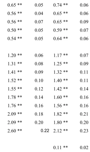
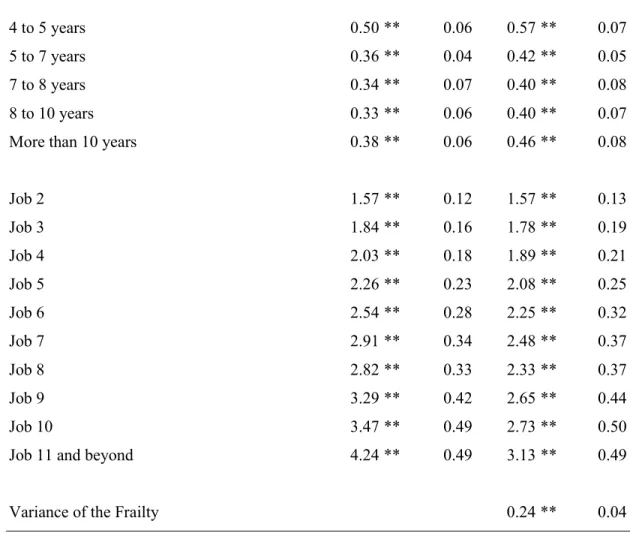
Table 7 shows that among workers in their first job, those who earn 30-50% above the average wage rate face a 70% higher risk of being laid off than workers earning just the average wage rate. The distinction across jobs is also relevant in the context of involuntary job separations. By the fifth job, workers earning 50% above the market wage rate are only 50% more likely to experience a layoff, while workers in their tenth job are as likely of experiencing a layoff as workers earning just the average market wage rate. Again, the informational content embedded in ε declines for more experienced workers. As the worker becomes more experienced and accumulates a large number of jobs, the employer is more likely to find additional sources of information about the worker such as references from previous employers.

To summarize my results, I find that workers voluntarily leave their jobs whenever they find themselves being paid below the customary wage rate. A worker who earns 30% less than what he expects to be earning according to his characteristics and labor market experience, is more than one and a half times as likely to initiate a separation. This result is consistent across models. As expected non-monetary rewards like employer provided health insurance substantially reduces the risk of initiating a job separation.

The distinction between voluntary and involuntary job separations seems to be relevant. Separate estimations for the hazard of voluntary separations and layoffs reveal that both processes indeed look different with respect to most of the covariates introduced in the model. The risk of being laid off is an increasing function of the size of the residual. Workers in the tenth decile face an almost 50% higher risk of being laid-off than workers earning the market wage rate.

I have also shown that the informational content on the residual seems to decline as the worker acquires more experience (and presumably he learns more about his true productivity) or as the employer information sources increase. I fitted two different models. In the first one, the coefficient of the residual is allowed to vary across job number. In the second one, the coefficient of the residual is allowed to vary across pre-experience levels. In both models, the absolute value of the residual coefficient decreases, but it is still statistically different from zero, as experience or the number of jobs increase. The information embedded in the residual, though, seems to be discounted at higher experience levels.

5.

WAGE MOBILITY THROUGH JOB MOBILITY

In Section 4.2, I showed that workers earning significantly below the market wage are more likely to quit their jobs while workers earning above the market wage rate face a higher risk of being laid-off. This effect persists even after controlling for heterogeneity or the natural propensity of the individual to move. Controlling for heterogeneity allows us to account for individual preferences about mobility.

There has been much discussion in the literature concerning what the returns to mobility are and how to measure them. Most of the emphasis has been on comparing wage growth between movers and stayers. In general the comparison is made using a wage regression in which the dependent variable is wage growth and the independent variables are human capital variables and dummy variables reflecting worker mobility patterns.

Following the ideas sketched in Section 2.2, I will take a different and simpler approach. Recall that expression (9) gave us the estimated residual value of the workers current job. That is, εit >0

means that the worker is earning above his expected wage rate at time t, while _{εit <}0 indicates that the worker is earning below his expected wage rate. Then, if on average workers improve their relative position through job changing we might be able to conclude that job mobility is a good thing, while if on average workers who move experience moves to the left of the distribution we should conclude that job mobility does not pay. Others ad hoc directional indices can be used, such as the fraction of upward or downward movers20.

Take the workers relative position _ε at time t and compare it with the worker’s relative position when he is observed at a new job at t+_δ. Then, we calculate _εt+δ −_εt for each job separation. As both _εt+δ and _εt give us the relative position of the worker at each point in time on their wage offer distribution, we can see _εt+δ −_εt as the relative gain from the job change. As I explained in Section 2.2, in terms of Figure 1, I should observe quitters moving to the right in their corresponding wage offer distribution. On the contrary, laid-off workers should lose ground after experiencing the job separation.

Voluntary job changes lead, on average, to gains in the order of 7%, while layoffs imply losses of 5%. These gains are estimated taking into account only those job-to-job changes that take place within a six-month period. Table 8 shows the distribution of job changes by the time elapsed between jobs. There, we can see that almost 90% of the voluntary job separations end in employment within a six-month period. This notably contrasts with involuntary job changes. Less than 75% of the laid-off workers find a job within a six-month period. The estimated mobility gain also depends on the subset of job changes considered. The longer the time between jobs, the smaller the gains from the job change. In what follows, I am going to use only those job changes that end in employment within a six-month period.

One must be careful in interpreting these estimated gains/losses. The residual might grow or fall purely as a statistical matter. If the risk of quitting is particularly high for those with big negative residuals, regression to the mean implies that the future residual for quitters will be bigger on average. We should find the opposite for laid-off workers. That is, relative gains/losses depend on the initial position of the worker. Figure 9 plots average wage gains by the decile location of each observation. It is clear that independently of the decile location of each job, jobs left voluntarily imply higher gains than jobs left involuntarily. For the three groups, workers who have the most to gain from the move experience the higher gains. Part of this is regression to the mean, but regression towards the mean is not the whole story. Both types of movers, quitters and laid-off workers experience different gains at the different residual deciles. Table 9 presents the average gains by residual decile and mobility status with corresponding confidence intervals.

Figure 10 plots the distribution of wage gains conditionally on mobility type. As I expected, stayers generally remain fairly stationary with respect to their offer distribution. Although quitters have positive wage gains on average, a fairly high amount of quits (30%) end up with wage losses. Quitting seems to be a risky, but very rewarding activity. Following Fields (2001) I can also use the familiar criterion of stochastic dominance to inspect the relationship between gains and looses of the different mobility types. Figure 11 plots the cumulative distribution of wage gains for the different mobility types.

Workers should not expect, though, for voluntary mobility to be rewarded uniformly at these high rates throughout their entire career. There seems to be a right time to move and collect wage gains. Figure 12 plots the average wage gains by selected labor market experience levels. There, we

can see that while workers in their first year in the labor market can expect to earn 15% after voluntarily changing jobs, the expected gain falls by half by the tenth year in the labor market. Laid-off workers losses, on the contrary, do not present a clear pattern. Table 10 presents the corresponding average wage gains and confidence intervals.

Expected gains fall more for highly skilled workers than for less skilled workers. After examining wage gains across educational levels and experience I find that while highly educated workers experience large wage gains from job mobility early in the career, these gains seems to vanish late in the career. In Figure 13, I plot wage gains by labor market experience for both High School and College Graduates. Early in the career, college graduates receive wage gains 30% higher than high school graduates. By the tenth year of the career college graduates see their wage gains vanish, while high school graduates still experience small (statistically significant) wage gains. Laid-off college graduates, in contrast, systematically experience average wage losses of 5-20% through their whole career.

Table 11 presents the average wage gains by mobility status and by the predicted hazard of experiencing a voluntary separation. The more likely the worker is to initiate a job separation, the more he gains when he decides to move. Figure 14 plots the average gains against the hazard of experiencing a voluntary job separation (columns 2, 4 and 6 in Table 11). I find that independent of the probability of initiating a separation, workers that choose to move do not experience loses. Average mobility returns for quitters are not statistically different from zero for workers with a low probability of quitting. Quitters do much better than both stayers and laid-off workers, though, when they are able to anticipate the move.

Note that among stayers and laid-off workers, only those with a high probability of initiating a separation experience wage gains. Stayers with high quit probabilities might be those who successfully negotiate their continued employment with the firm. They do not gain as much as the workers that choose to quit, but presumably they do not suffer the non-monetary cost of quitting. On the contrary, laid-off workers with high quit probabilities might be the ones who unsuccessfully tried to negotiate their continued employment with the firm.

Table 12 presents average wage gains by mobility status and the predicted hazard of experiencing a layoff. The wage gains of both stayers and quitters are not systematically related to the probability of being laid-off. The wage gains of quitters are all either positive or not statistically different from zero, while wage gains of stayers are only statistically different from zero for the group of workers in the highest decile of the predicted hazard distribution. Laid-off workers, in contrast, systematically suffer wage loses. Moreover, larger losses are experienced by the workers with the higher probability of being laid-off. Again, note that part of this effect may be due to regression towards the mean. Workers with the high probabilities of being laid-off are at the same time the workers with the largest residuals and, therefore the ones that have the most to lose.

In this Section, I have shown that voluntary mobility does pay. Workers who choose to change jobs experience mobility gains on the order of 7%. Laid-off workers tend to perform poorly relatively to quitters and stayers and suffer average losses of 5%.

The size of the wage gains associated with the job mobility behavior is strongly tied to the worker’s skill accumulation. While at early stages of the career workers experience large wage gains from quitting, these gains seems to disappear as the career extends. College Graduates are the ones who experience the biggest proportional losses. Laid-off losses increase as the career extends, particularly for high-skilled workers. Mobility gains are also affected by gaps in employment. Wh