No. 469
Three-structured smooth transition
regression models based on CART
algorithm
Joel Corrêa da Rosa
Álvaro Veiga
Marcelo C. Medeiros
TEXTO PARA DISCUSSÃO
DEPARTAMENTO DE ECONOMIA
www.econ.puc-rio.br
DEPARTAMENTO DE ECONOMIA
PUC-RIO
TEXTO PARA DISCUSSÃO
N
o. 469
T
REE
-S
TRUCTURED
S
MOOTH
T
RANSITION
R
EGRESSION
M
ODELS
B
ASED ON
CART A
LGORITHM
JOEL CORRÊA DA ROSA
ÁLVARO VEIGA
MARCELO C. MEDEIROS
JANEIRO 2003
(revised)
ALGORITHM
JOEL CORR ˆEA DA ROSA, ALVARO VEIGA, AND MARCELO C. MEDEIROS
ABSTRACT. The goal of this paper is to introduce a tree-based model that combines aspects of CART (Classi-fication and Regression Trees) and STR (Smooth Transition Regression). The model is called the Smooth Tran-sition Regression Tree (STR-Tree). The main idea relies on specifying a parametric nonlinear model through a tree-growing procedure. The resulting model can be analyzed as a smooth transition regression with multiple regimes. Decisions about splits are entirely based on a sequence of Lagrange Multiplier (LM) tests of hypothe-ses. An alternative specification strategy based on a 10-fold cross-validation is also discussed and a detailed Monte Carlo experiment is carried out to evaluate the performance of the proposed methodology in comparison with standard techniques. The STR-Tree model outperforms CART when the correct selection of the architec-ture of simulated trees is considered. Furthermore, the LM test seems to be a promising alternative to 10-fold cross-validation. When put into proof with real datasets, the STR-Tree model has a superior predictive ability than CART.
KEYWORDS. Regression-trees, CART, smooth transitions, nonlinear models, regression, modelling cycle, pre-diction.
1. INTRODUCTION
IN RECENT YEARSmuch attention has been devoted to nonlinear modelling. Techniques such as artifi-cial neural networks, nonparametric regression and recursive partitioning methods are frequently used to approximate unknown functional forms. In spite of their success in various applications, frequently these approaches lack interpretability due to the complexity of the final model. Some cases in which the fitted model can be given a reasonable interpretation, there are no inferential procedures that guarantee the sta-tistical significance of the parameters. The proposal of the present paper is the construction of a nonlinear regression model that combines aspects of two well-known methodologies: Classification and Regression Trees (CART) discussed in Breiman, Friedman, Olshen, and Stone (1984) and the Smooth Transition Re-gression (STR) presented in Granger and Ter¨asvirta (1993), by taking advantages of their main capabili-ties. Our model inherits from CART the simplicity and interpretability of the tree-based models while the STR framework provides tools for inference-based decisions. The proposed model is called the Smooth Transition Regression Tree (STR-Tree). The CART methodology represents a unification of all tree-based Date: January 14, 2004.
classification and prediction methods that have been developed since a first approach presented by Morgan and Sonquist (1963). It transformed the regression tree models in an important nonparametric alternative to the classical methods of regression. Since then, the attractiveness of this methodology has motivated many authors to create hybrid modelling strategies that merge tree techniques with known statistical methods. See, for example, Segal (1992) in a context of longitudinal data analysis, Ahn (1996) for survival analysis, and Cooper (1998) for time series analysis. Other approaches can be found in Ciampi (1991), Crowley and Blanc (1993), and Denison, Mallik, and Smith (1998).
In our proposal, by allowing smooth splits on the tree nodes instead of sharp ones, we associate each tree architecture with a smooth transition regression model and thus it turns possible to formulate a splitting criteria that are entirely based on statistical tests of hypotheses. The Lagrange Multiplier (LM) test in the context presented by Luukkonen, Saikkonen, and Ter¨asvirta (1988) is adapted for deciding if a node should be split or not1. Here, the tree growing procedure is used as a tool for specifying a parametric
model that can be analyzed either as STR model or as a fuzzy regression (Jajuga 1986). In the former case, we can obtain confidence intervals for the parameters estimates in the tree leaves and predicted values. Decisions based on statistical inference also lessen the importance of post-pruning techniques to reduce the model complexity. An alternative specification strategy based on a 10-fold cross-validation is considered. An extension of the basic model to allow for the inclusion of categorical variables is also discussed. A detailed Monte Carlo experiment is carried out to evaluate the performance of the proposed methodology in comparison with standard techniques. The STR-Tree model outperforms CART when the correct selection of the architecture of simulated trees is considered. Furthermore, the LM test seems to be a faster and promising alternative to 10-fold cross-validation. When put into proof with real datasets, the STR-Tree model has a superior predictive ability than CART. A Matlab code for carrying out the modelling cycle exists and can be obtained from the authors.
The paper is divided as follows. In Section 2, we briefly introduce some important regression tree con-cepts and introduce the main notation. Section 3 brings the proposal of a tree-structured smooth transition regression. Section 4 discusses the model building strategy and parameter estimation. The use of categori-cal data is considered in Section 5. A Monte Carlo Experiment to evaluate the estimators properties and the ability of the sequence of LM-type tests to identify right-sized trees is performed in Section 6. Examples with five datasets are presented in Section 7. Finally, Section 8 concludes. A technical appendix provides the proofs of the theorems.
1See Ter¨asvirta (1994), van Dijk, Ter¨asvirta, and Franses (2002), and the references therein for successful applications of similar
2. REGRESSIONTREES
A regression tree is a nonparametric model which looks for the best local prediction, or explanation, of a continuous response through the recursive partitioning of the space of the predictor variables. The fitted model is usually displayed in a graph which has the format of a binary decision tree with parent and terminal nodes (also called leaves), and which grows from the root node to the terminal nodes. For example, Figure 1 displays a tree with three parent nodes and four leaves.
2.1. Mathematical Formulation. Letxt = (x1t, . . . , xmt)0 ∈ X ⊆ Rmbe a vector which containsm
explanatory variables for a continuous univariate responseyt ∈ R. The relationship betweenytandxt
follows the regression model
yt=f(xt) +εt, (1)
where the functional form f(·) is unknown and there are no assumptions about the distribution of the random termεt. Following Lewis and Stevens (1991), a regression tree model withKleaves is a recursive
partitioning model that approximates f(·) by a general nonlinear function H(xt;ψ)of xt and defined
by the vector of parametersψ ∈ Rr; r is the total number of parameters. UsuallyH(·)is a piecewise constant function defined byKsubregionski(θi),i= 1, . . . , K, of some domainK⊂Rm. Each region is
determined by the parameter vectorθi,i= 1, . . . , K, such that
f(xt)≈H(xt;ψ) = K X i=1 βiIi(xt;θi), (2) where Ii(xt;θi) = 1 ifxt∈ki(θi); 0 otherwise. (3) Note thatψ =¡β1, . . . , βK,θ01, . . . ,θ0K ¢0
. Conditionally to the knowledge of the subregions, the rela-tionship betweenytandxtin (1) is approximated by a linear regression on a set ofKdummy variables.
Figure 1 illustrates the features of a model provided by a regression tree that explains the relationship between a response variableyand a set of two explanatory (predictor) variablesx1andx2. The predicted
values foryare obtained through a chain of logical statements that split the data into four subsets.
The most important reference in regression tree models is the CART approach discussed in Breiman, Friedman, Olshen, and Stone (1984). In this context, it is usual to define the subregionski,i= 1, . . . , K,
in (2) by hyperplanes that are orthogonal to the axis of the predictor variables; see Figure 1. For example, consider the simplest tree structure withK= 2leaves and depthd= 1as illustrated in Figure 2.
FIGURE1. Graphical Display of a Regression Tree.
FIGURE2. Simplest tree structure.
The unknown functionf(xt)in (1) may be approximated by a constant model in each leaf, written as
yt=β1I(xt;s0, c0) +β2[1−I(xt;s0, c0)] +εt, (4) where I(xt;s0, c0) = 1 ifxs0t≤c0; 0 otherwise, (5) ands0∈S={1,2, . . . , m}.
To mathematically represent more complex tree structures, we adopt a labeling scheme which is similar to the one used in Denison, Mallik, and Smith (1998). The root node is at position0and a parent node at positionjgenerates the left-child node and right-child node at positions2j+ 1and2j+ 2, respectively. Consider a tree withNparent nodes. The variablesxsj,j= 1, . . . , Nare usually called splitting variables.
The notation presented in this section will be used thorough the paper. More complex trees are shown in the following examples.
FIGURE3. Regression tree with three terminal nodes representing (6).
FIGURE4. Regression tree model with four terminal nodes representing (7).
EXAMPLE1. Consider a regression tree defined by
yt={β3I(xt;s1, c1) +β4[1−I(xt;s1, c1)]}I(xt;s0, c0)+
β2[1−I(xt;s0, c0)] +εt.
(6)
A graphical representation of (6) is illustrated in Figure 1. The tree induced by (6) has two parent nodes, three terminal nodes (leaves), and the depth is equal to two.
EXAMPLE2. Consider the following regression tree:
yt={β3I(xt;s1, c1) +β4[1−I(xt;s1, c1)]}I(xt;s0, c0)+
{β5I(xt;s2, c2) +β6[1−I(xt;s2, c2)]}[1−I(xt;s0, c0)] +εt.
(7)
A graphical representation of (7) is illustrated in Figure 2. Model (7) has three parent nodes, four leaves, and depth 2.
Details about the tree growing procedure and the CART algorithm is presented in Breiman, Friedman, Olshen, and Stone (1984).
3. TREE-STRUCTUREDSMOOTHTRANSITIONREGRESSION(STR-TREE)
The main idea of the STR-Tree model is to take advantage of much of the CART structure presented in Section 2, but also to introduce elements which make it feasible to use standard inferential procedures. We intend to keep the interpretability of the tree-based models but to analyze them as a class of parametric nonlinear models. The highly discontinuous functional form of the model fitted by the CART and the strategy to decrease the sum of squared errors by splitting the sample recursively, pose a problem to test the significance of the model and to make classical inference. The idea here is the same used in Su´arez and Lutsko (1989): the substitution of sharp splits in the CART model by smooth splits. Consider the simplest tree with two terminal nodes generated as in (4). If we replace the indicator functionI(·)in (4) by a logistic function defined as G(xt;s0, γ0, c0) = 1 1 +e−γ0(xs0t−c0), (8) we obtain yt=β1G(xt;s0, γ0, c0) +β2[1−G(xt;s0, γ0, c0)] +εt, (9)
where now we have the additional parameterγ0, called the slope parameter, which controls the smoothness
of the logistic function. This change causes an important difference from the CART approach: splitting the root node will not separate two subsets of observations but it will create two fuzzy sets (Zadeh 1965) where all observations will belong to, but with a different degree of membership. Note that the CART node partition is nested in the smooth transition approach as a special case obtained when the slope parameter approaches infinity. On the other hand, when the slope parameter approaches zero, it leads to the fuzziest situation in which there is no gain in splitting the data. The parameterc0is called the location parameter.
Assuming that the error term is a random variable with a known probability distribution, from (8) and (9) it becomes possible, without loosing the flexibility of the CART approach, to interpret the regression tree approach as a particular case of the STR models discussed in Granger and Ter¨asvirta (1993) and Ter¨asvirta (1998)2.
2The STR-Tree model has also some similarities with the Multiple-Regime Smooth Transition Autoregressive (MRSTAR) model
4. MODELBUILDING
The tree growing process of the STR-Tree model is an adaptation of the modelling cycle described in Ter¨asvirta (1994) and Ter¨asvirta (1998). As mentioned in the introduction, our goal is to build a coherent strategy to grow the STR-Tree model using statistical inference. The “architecture” of the model has to be determined from the data and we call this stage specification of the model, which involves two decisions: the selection of the node to be split and the index of the splitting variable. The specification stage will be carried out by sequence of Lagrange Multiplier (LM) tests following the ideas originally presented in Luukkonen, Saikkonen, and Ter¨asvirta (1988). An alternative approach based on 10-fold cross-validation is also possible; however the computational burden involved is dramatically high. See Sections 6 and 7 for further details. The specification stage also requires estimation of the parameters of the model. What follows thereafter is evaluation of the final estimated model. Tree models are usually evaluated by their out-of-sample performance (predictive ability). In this paper we follow the literature and evaluate the STR-Tree model in the same way. The construction of misspecification tests for the STR-STR-Tree model in the same spirit of Eitrheim and Ter¨asvirta (1996) is also possible, but this topic is beyond the scope of the paper.
Following the “specific-to-general” principle, we start the cycle from the root node (depth 0) and the general steps are:
(1) Specification of the model by selecting in the depthd, using the LM test, a node to be split (if not in the root node) and a splitting variable.
(2) Estimation of the parameters of the logistic function and the constants within the nodes. (3) Evaluation of the estimated model by checking if it is necessary to:
(a) Change the node to be split. (b) Change the splitting variable. (c) Remove the split.
(4) Use the final tree model for prediction or descriptive purposes.
Figure 5 illustrates the cycle. The modelling cycle begins from the root node (depth 0) by testing the null hypothesis of a global constant model against the simplest STR-Tree model which contains 2 terminal nodes.
FIGURE5. Modelling cycle of STR-Tree model.
4.1. Parameter Estimation. Consider a full-grown STR-Tree model with depthd,K= 2dterminal nodes
(leaves), andN =Pdi=12iparent nodes, defined as
yt=H(xt;ψ) = K
X
k=1
βK+k−2Bk(xt;θk) +εt, (10)
whereBk(xt;θk),k = 1, . . . , K, is defined by products of the logistic function. The parameter vector
ψ =¡βK−1, . . . , β2K−2,θ01, . . . ,θ0K
¢0
hasr=K+ 2N elements. As an example, for a tree architecture as in Figure 5, the STR-Tree model has depthd = 2, K = 4, N = 3, and the functionsBk(xt;θk),
k= 1, . . . , K, in (10) are written as
B1(xt;θ1) =G(xt;s0, γ0, c0)G(xt;s1, γ1, c1) ;
B2(xt;θ2) =G(xt;s0, γ0, c0) [1−G(xt;s1, γ1, c1)] ;
B3(xt;θ3) = [1−G(xt;s0, γ0, c0)]G(xt;s2, γ2, c2) ;and
B4(xt;θ4) = [1−G(xt;s0, γ0, c0)] [1−G(xt;s2, γ2, c2)].
The total number of parameters to be estimated is10and there are three splitting variables to be selected. 4.2. Main Assumptions and Asymptotic Theory. At this point we have to make the following set of assumptions.
ASSUMPTION1. The sequence{xt}Tt=1is formed by independent and identically distributed (IID) random
vectors and have a common joint distributionDon∆, a measurable Euclidean space, with measurable Radon-Nikod´ym density.
ASSUMPTION2. The sequence{εt}Tt=1is formed by independent and normally distributed (NID) random
variables with zero mean and varianceσ2<∞,εt∼NID
¡ 0, σ2¢.
ASSUMPTION3. Ther×1true parameter vectorψ∗is an interior point of the compact parameter space
Ψwhich is a subspace ofRr, ther-dimensional Euclidean space.
ASSUMPTION4. The parametersγi>0,i= 1, . . . , N, whereNis the number of parent nodes.
Further-more, if for two adjacent parent nodes at positions2j+1and2j+2,xs2j+1t=xs2j+2t, thencs2j+1< cs2j+2.
Assumption 1 states that we are working with IID data such as cross-sectional or a set of time-series with IID observations. Although Assumption 2 may seem, in principle, a little restrictive, model (10) is still very flexible. Furthermore, Assumption 2 allows us to work in a maximum likelihood framework that will be equivalent to nonlinear least-squares. In the case of non-Gaussian errors, Assumption 2 may be substituted by some moment conditions and a quasi-maximum likelihood framework should be used instead. The main difference will be related to the computation of the covariance matrix of the parameter estimates. In addition, a robust version of the tests presented latter can be constructed in the same spirit of Medeiros, Ter¨asvirta, and Rech (2002), using the results developed in Wooldridge (1991). Assumption 3 is standard and Assumption 4 guarantees that the STR-Tree model is identifiable.
As discussed previously, we estimate the parameters of our STR-Tree model by maximum likelihood (ML) making use of the assumptions made ofεt. The use of maximum likelihood makes it possible to obtain
an idea of the uncertainty in the parameter estimates through (asymptotic) standard deviation estimates. The STR-Tree model is similar to many linear or nonlinear models in that the information matrix of the log-likelihood function is block diagonal in such a way that we can concentrate the log-likelihood and first estimate the parameters of the conditional mean. Conditional maximum likelihood is thus equivalent to nonlinear least squares (NLS).
The nonlinear least squares estimator (NLSE) of the parameters equals
b ψ=argmin ψ∈Ψ QT(ψ) =argmin ψ∈Ψ T X t=1 qt(ψ), (11) whereqt(ψ) = [yt−H(xt;ψ)]2.
Next, we discuss the existence, consistency, and asymptotic normality of the NLSE defined in (11).
4.2.1. Existence. The proof of existence of the NLSE is based on Lemma 2 of Jennrich (1969), which establishes that under certain conditions of continuity and measurability on the mean square error (MSE) function, the NLSE as in (11) exists. Theorem 1 state the necessary conditions for the existence of the NLSE.
THEOREM1. The STR-Tree model satisfies the following conditions and the NLSE exists.
(1) For eachxt∈X⊆Rm, functionHx(ψ) =H(xt;ψ)is continuous in compact subsetΨof the
Euclidean space.
(2) For eachψ∈Ψ⊆Rr, functionHψ(X) =H(xt;ψ)is measurable in spaceX.
(3) εtare errors independent and identically distributed with mean zero and varianceσ2.
4.2.2. Consistency. The consistency of the NLSE was rigorously proved in Jennrich (1969) and Malinvaud (1970). The former proves strong consistency while the latter weak consistency. Weak consistency is more common in the literature and is often called by the simpler name of consistency. The main reason why strong consistency, rather than weak consistency, is proved is that the former implies the latter and is often easier to prove. We follow the results presented in Amemiya (1983) and state the following theorem that gives the conditions under which the NLSE defined in (11) is strong consistent.
THEOREM2. Under the Assumptions 1–5 the NLSEψb is strong consistent forψ∗, i.e.,ψb a.s.→ ψ∗.
4.2.3. Asymptotic Normality. Asymptotically normality of the NLSE was also carefully proved in Jennrich (1969). We follow his results and the developments in Amemiya (1983) and state the following theorem.
THEOREM3. Under the Assumptions 1–5 T1/2( ˆψ−ψ∗) d →N µ 0,−plim T→∞ A(ψ∗)−1 ¶ , (12) whereA(ψ∗) =σ21T ∂2Q T(ψ∗) ∂ψ∂ψ0 .
REMARK1. The extension of the above theorems to the case of non-IID observations and to misspecified models is relatively straightforward. The results of White (1982), White (1994), and Wooldridge (1994) can be applied.
4.2.4. Concentrated Least-Squares. Conditional on the knowledge of the parameters θk in (10), k =
1, . . . , K, model (10) is just a linear regression and the vector of parametersβ = (βK−1, . . . , β2K−2)0
can be estimated by ordinary least-squares (OLS) as b β= [B(θ)0B(θ)]−1B(θ)0y, (13) wherey= (y1, . . . , yT)0,θ= ¡ θ01, . . . ,θ0K¢0, and B(θ) = B1(x1;θ1) · · · BK(x1;θK) .. . . .. ... B1(xT;θ1) · · · BK(xT;θK) .
The parametersθk,k= 1, . . . , K, are estimated conditionally onβby applying the Levenberg-Marquadt
algorithm which completes theith iteration. As the NLS algorithm is sensitive to the choice of starting-values, we suggest the use of a grid of possible starting-values.
4.3. Splitting the Nodes. We have a particular interest in the hypothesis concerning the significance of splitting the root node. If we re-parameterize the model defined by (8)–(9) as:
yt=φ0+λ0G(xt;s0, γ0, c0) +εt, (14)
whereφ0=β2andλ0=β1−β2, we obtain a more parsimonious representation of the simplest STR-Tree
model 3. In order to test the significance of the first split, a convenient null hypothesis isH0 : γ0 = 0
against the alternativeHa : γ0 >0. An equivalent null hypothesis isH00 : λ0 = 0. However, it is clear
in (14) that underH0, the nuisance parametersλ0 andc0 can assume different values without changing
3It becomes easier to note that (14) is a particular case of a neural network model with a single hidden layer (Hornik, Stinchombe, and
the likelihood function. This poses an identification problem whose solution was first discussed by Davies (1977). See also Davies (1987).
We adopt as a solution for this problem the one proposed in Luukkonen, Saikkonen, and Ter¨asvirta (1988)4, that is to approximate the functionG(·)by a third-order Taylor expansion aroundγ = 0. After some algebra we get
yt=α0+α1xs0,t+α2x 2
s0,t+α3x 3
s0,t+et, (15)
whereαi,i= 0,1,2,3, is a parameter that is function ofγ0,c0,φ0, andλ0,et=εt+λ0R(xt;s0, γ0, c0),
andR(xt;s0, γ0, c0)is the remainder.
Thus, the null hypothesis becomes
H0: αi= 0, i= 1,2,3. (16)
Note that underH0, the remainder of the Taylor expansion vanishes andet=εt, so that the properties
of the error process remain unchanged under the null and thus asymptotic inference can be used. Finally, it may be pointed out that one may also view (15) as resulting from a local approximation to the log-likelihood function, which for observationttakes the form
lt=−1 2ln (2π)− 1 2lnσ 2− 1 2σ2 © yt−α0−α1xs0,t−α2x 2 s0,t−α3x 3 s0,t ª2 . (17)
At this point we make the following additional assumption to accompany the previous Assumptions (2)–(4).
ASSUMPTION5. E|xs0t|
δ <∞,∀s
0∈S, for someδ >6.
This enables us to state the following well-known result.
THEOREM4. UnderH0:γ0= 0and Assumptions (2)–(5), the LM type statistic
LM= 1 b σ2 T X t=1 b εtν0t T X t=1 νtν0t− T X t=1 νth0t à T X t=1 hth0t !−1 T X t=1 htν0t T X t=1 νtεbt, (18)
wherebεt =yt−βb0is the estimated residuals under the null,bσ2 = (1/T)
PT t=1εbt2,ht = 1, andνt = ¡ xs0t, x 2 s0t, x 3 s0t ¢0
, has an asymptoticχ2distribution with3degrees of freedom.
REMARK2. Note that, underH0,βb0= T1
PT
t=1yt p
→E(yt).
Until this point, we have just interpreted the simplest tree model as a particular case of the STR model as in Granger and Ter¨asvirta (1993) and the testing strategy to split the root node corresponds to a linearity test in which the linear model in question is a global constant model. However, the key idea is to consider the basic testing procedure described above in a more complex framework. To give an example of a more complex model, consider that the null hypothesis (16) was rejected and a STR-Tree model with two leaves was consistently estimated. A natural way, within the tree framework, of considering a hypothesis of misspecification is by formulating a new model that splits one between the two created nodes, say the left child node, leading to the following model
yt=H(xt;ψ) +εt ={β3G(xt;s1, γ1, c1) +β4[1−G(xt;s1, γ1, c1)]}G(xt;s0, γ0, c0)+ β2[1−G(xt;s0, γ0, c0)] +εt. (19) Therefore, rewriting (19) as yt= [φ1+λ1G(xt;s1, γ1, c1)]G(xt;s0, γ0, c0)+ β2[1−G(xt;s0, γ0, c0)] +εt, (20)
whereφ1=β3andλ1=β3−β4, a convenient null hypothesis isH0: γ1= 0.
However, under the null hypothesis, the model (20) can not be consistently estimated because of the nui-sance parametersλ1andc1. For solving this identification problem, we proceed as before and approximate
the functionG(·)by its third-order Taylor expansion aroundH0. After some algebra we get
yt=α0+α1G(xs0t;γ0, c0) +α2G(xs0t;γ0, c0)xs1t+ α3G(xs0t;γ0, c0)x 2 s1t+α4G(xs0t;γ0, c0)x 3 s1t+et, (21)
whereet =εt+R(xt;s1, γ1, c1);R(xt;s1, γ1, c1)is the remainder. The decision for splitting the node
corresponds to the rejection of the following null hypothesis
H0: αi= 0, i= 2,3,4. (22)
The test statistic is (18) with
ht= ∂H(xt;ψ) ∂ψ0 ¯ ¯ ¯ ¯ ¯ H0 = Ã 1, G(xs0t;bγ0,bc0), ∂G(xs0t;γ0, c0) ∂γ0 ¯ ¯ ¯ ¯ ¯ H0 , ∂G(xs0t;γ0, c0) ∂c0 ¯ ¯ ¯ ¯ ¯ H0 !0 (23)
and νt= ¡ G(xs0t;γb0,bc0)xs1t, G(xs0t;bγ0,bc0)x 2 s1t, G(xs0t;bγ0,bc0)x 3 s1t ¢0 . (24)
From the assumption of normality of the error term, the information matrix is block diagonal and thus we can assume that the error variance is fixed. If we use the F-version of the LM-type test, from the score vector, under the null hypothesis, we can see that the decision statistic may be calculated according to the following steps:
(1) Estimate the STR-Tree model under the null hypothesisH0and compute the residualsbεt. Compute
the sum of the squared residualsSSR0=
PT t=1εb2t.
(2) Regressbεtonhtandνt. Compute the sum of squared residuals obtained from this regression,
SSR1=
Pt
t=1ub2t.
(3) Compute theχ2statistic
LMχ=T
SSR0−SSR1
SSR0
, (25)
or theFversion of the test
LMF =
(SSR0−SSR1)/3
SSR1/(T−7)
, (26)
whereT is the sample size. Under the nullLMχ is asymptotically distributed as aχ2distribution
with 3 degrees of freedom andLMFhas an asymptoticFdistribution with3andT−7degrees of
freedom.
Hereafter, the idea is to carry out a sequence of LM-type tests to grow the tree model in the same format as the one presented above and the general form of the test statistic when testing a model withjnodes against an alternative withj+ 1nodes is given by:
LM = (SSR0−SSR1)/3
SSR1/[T−(p+ 3)]
, (27)
wherepis the total number of elements of the vectorht.
The modelling strategy is described in the following sections.
4.3.1. Modelling Cycle from the root node (depth 0). The decision to split the root node is based on the following steps.
(1) For each explanatory variable, apply the LM-type test described above and select the variablexs0t
(2) Conditional to the choice ofs0, estimate the vector of parametersψ= (γ0, c0, β1, β2)0by
concen-trated QML.
(3) Evaluate the estimated model by testing the hypothesis (conditional onγ0andc0)
H01: β1= 0
H02: β2= 0
H03: β1−β2= 0|β1, β26= 0
(28)
against bilateral alternatives. If at least one among the evaluated hypothesis do not reject the null, the cycle returns to the specification stage and the next splitting variable attached to the ranking of
p-values is selected. In case of all candidates variables do not produce a significant split, the root node is declared as terminal and the global constant model is selected as the best model. Otherwise, two children nodes are generated to compose the first depth of the tree.
4.3.2. Modelling Cycle from the 1st depth. After the tree has started to grow from the root node, the first depth is created and the cycle continues by testing for the adequacy of splitting one between the two children nodes. The null hypothesis in this test concerns the conditional linear model and the alternative brings the inclusion of a nonlinear term that is responsible for splitting the node. From now on, besides selecting a splitting variable, we shall also select which one between the two created nodes shall be split at the first place.
(1) For each combination of splitting variable index inS ={1,2, . . . , m}and node number inD1=
{1,2}, apply the LM-type test and select the indexesj1∈D1andsj1 ∈Sthat generates the lowest
p-value below a pre-specified significance level. (2) Estimate the parameters of the model.
(3) We evaluate the model by testing the null hypothesis: H01: β2j1+1= 0
H02: β2j1+2= 0
H03: β2j1+1−β2j1+2= 0|β2j1+1, β2j1+26= 0
(29)
Without finding significance in all tests above, the model has to be re-specified by choosing a new combination of a node and splitting variable index. If the split is accepted, then the cycle returns to the1st step by applying the LM test for testing the model with 3 terminal nodes against the alternative that splits the nodej2∈D1− {j1}. The2nd depth will be complete whether both nodesj1andj2produce significant
splits. In case ofj1to be the only node to generate children nodes, the2nd depth will be composed of two
nodes whose numbers are2j1+ 1and2j1+ 2. If there is no significant split, the tree growing process stops.
4.3.3. Modelling Cycle from thekth depth. The execution of the algorithm in a general depthkis straight-forward.
(1) Apply the LM test to all combinations of splitting variables indexes and nodes in the set Dk
which contains all numbers of children nodes that compose the kth depth. Note that Dk ⊆
©
2k−1,2k, . . . ,2k+1−2ª.
(2) Selectj1∈Dkandsjk ∈Sby the rank of significantp-values obtained through the LM-type test.
(3) Estimate the parameters of the model.
(4) Evaluate the model by checking thet-values of the constants within the generated nodes and the significance of the difference between them. The cycle in this depth is executed iteratively by testing, and if necessary, splitting the nodes according to the sequence:
j2∈D1− {j1}
j3∈D1− {j1, j2}
j4∈D1− {j1, j2, j3}
· · ·
Reaching a point in which there is no more significant splits, the algorithm is addressed to work on the (k+ 1)th depth. The whole cycle ends when a determined depth do not produce children nodes.
4.4. Sequential Tests. To achieve the final tree model, we perform a sequence ofncorrelated LM-type tests of hypothesis in whichnis a random variable. During this sequence, the harmful decision to be taken, according to the principle of tree-complexity as function of the number of terminal nodes, is to decide erroneously for splitting a node. Due to multiplicity from repeated significance testing, we have to control the overall type I error under the risk of an overstatement of the significance of the results (more splits are reported to be significant than it should be). To remedy this situation, we adopt the following procedure. For thenth test in the sequence, if it is performed in thedth depth the significance level isα(d, n) =nαd.
In the root node (d = 0)and we apply the first test (n = 1)for splitting the node at a significance levelα, if the null is rejected than we the second(n = 2)test is applied in the1st depth(d= 1)and the significance level isα/2. Then, if the tree grows by completing all depths, the significance level evolves likeα/3,α/42,α/52,α/63,α/73,α/84,α/94, etc. Figure 6 exhibits a hypothetical example of how could
FIGURE6. Significance level while testing for splitting the nodes - hypothetical example.
it be the evolution of the significance level during the tree growing process. The arrows in Figure 6 show the order in which the nodes are tested for splitting in each depth of the tree. By forcing the test to be more rigorous in deeper depths, we create a procedure that diminishes the importance of using post-pruning techniques.
There are several alternatives to control the overall size of the sequence of tests (Hochberg 1988, Ben-jamini and Hochberg 1995, BenBen-jamini and Hochberg 1997, BenBen-jamini and Yekutieli 2000, BenBen-jamini and Yekutieli 2001, Benjamini and Liu 1999). However, by our experiments, the simple methodology described above seems to work quite well and the comparison between different techniques to reduce the nominal size of each test is beyond the scope of the paper. In practice, different methodologies can be tested and possible different architectures may be compared by their out-of-sample performance.
5. CATEGORICALDATA
In principle the developments of the previous sections did not take into account the case where some of the variables are categorical. However, the extension to include categorical data is straightforward. The main idea is to replace the constant model in each terminal node by a linear regression on a constant and a set of dummy variables representing the categorical data.
Letxt= (z0t,wt0)0, wereztis a vector of categorical variables andwtis a vector of continuous variables.
In addition, letDt(zt)be a vector of dummy variables representing the categorical vectorzt. In that case
model (10) may be rewritten as:
yt=H(xt;ψ) = K
X
k=1
This is a similar approach as the one used in the STR literature to handle the presence of dummy regres-sors.
6. MONTECARLOEXPERIMENT
A Monte Carlo experiment was designed with two objectives. The first one is to study the small sample properties of the nonlinear least squares estimators for the parameters of the STR-Tree simulated models. The second is to investigate the performance of three different tree-growing algorithms:
CART:: We use the most traditional CART tree growing strategy. This consists of growing the
max-imum sized tree, using as a stopping rule the minmax-imum of five observations per terminal node, and then prune the tree using the 1-SE rule with errors estimates obtained by 10-fold cross validation.
STR-Tree/LM:: As described in previous sections, this strategy uses the LM type test to select
si-multaneously the node and splitting variable. This specification strategy does not need pruning and the control of the overall error is done by the reducing the test size during the tree growing.
STR-Tree/CV:: In a trial to use a strategy similar to CART one, we carry at each node a 10-fold
cross-validation experiment to select the splitting variable that minimizes the overall MSE (Mean Square of Errors) evaluated out-of-sample. When the MSE plus a standard error is greater than the one found in the previous split, the node is declared terminal.
We simulated two small tree architectures which are illustrated in Figure 7. By the selection of these two small tree architectures, which go beyond the smallest one which contains two nodes, we simulated models for different combinations of the smoothness parameters at the parent nodes. Thus, four models were simulated for Architecture I which contains three terminal nodes and two models were simulated for Architecture II which has four terminal nodes. Basically, we considered in Table 1 two types of splits, smooth(γi = 0.5) and sharp(γi = 5)that were mixed in different splitting sequences during the tree
growing. Model 1.1, for example, is obtained from two consecutive smooth splits and Model 1.4 brings a smooth split at the root node, followed by a sharp split.
(a) Architecture I (b) Architecture II
TABLE1. Smoothness of the splits in the STR-Tree simulations Model First Split Second Split Third Split Architecture I 1.1 γ0= 0.5 γ2= 0.5 — (3 leaves) 1.2 γ0= 5 γ2= 5 — 1.3 γ0= 5 γ2= 0.5 — 1.4 γ0= 0.5 γ2= 5 — Architecture II 2.1 γ0= 0.5 γ1= 0.5 γ2= 0.5 (4 leaves) 2.2 γ0= 5 γ1= 5 γ2= 5
There were 1000 replications for each model with sample sizesT = 150andT = 500, in a trial to repre-sent small and large samples. As the main concern was about the effects of the smoothness parameter, there was no much variation in the choice of the constants within the nodes. Three uncorrelated and normally distributed predictor variables were used as candidates to be the splitting variables: x1 ∼ N(10,2.56);
x2 ∼N(90,9); andX3∼N(25,4). The error term is defined asεt∼N(0,1). Since the smoothness
pa-rameter is not scale-free, we standardized the argument of the logistic function, dividing it by the standard deviation of the splitting variable. The other parameters were fixed according to Table 2.
TABLE2. Parameters in the simulated STR-Tree models Architecture I Architecture II Constants β1= 6 β3= 6;β4= 3.2 in the nodes β5= 1.8;β6=−1.5 β5= 1.8;β6=−1.5
Location parameters c0= 83;c2= 10 c0= 90;c1= 10;c2= 25
Indexes of splitting variables s0= 2;s2= 1 s0= 2;s1= 1;s2= 3
As shown in Table 2, the location parameters were chosen strategically at median points for simulations under Architecture II. The aim was to provide a minimum amount of information within the created nodes. The only concern related to the choice of the constants within the nodes was to yield different local models. From all combinations presented above, there are completely different relationship among the response variable and the set of explanatory variables.
Unlike CART that fits a multidimensional histogram to data, the STR-Tree model represents a surface fitting. The difference among models for Architecture I can be seen in in Figure 8 that brings the response surface for each one of the simulated trees. When all splits are sharp such as in model 1.2, the surface looks like a bivariate histogram. On the other hand, a sequence of extremely smooth splits (Model 1.1) produces a relationship between the response and regressors that is almost linear.
6.1. Parameter Estimation. In this Section, we present and discuss the empirical results obtained with the use of the NLSE in the simulated models. The results are described through descriptive statistics such as the sample mean and median for verifying the central tendency.
6 8 10 12 14 70 80 90 100 110 120 130 0 0.5 1 1.5 2 2.5 3 3.5 4 4.5 X2 X1 Y (a) Model 1.1 6 8 10 12 14 70 80 90 100 110 120 130 −2 −1 0 1 2 3 4 5 6 X2 X1 Y (b) Model 1.2 6 8 10 12 14 70 80 90 100 110 120 130 −1 0 1 2 3 4 5 6 X2 X1 Y (c) Model 1.3 6 8 10 12 14 70 80 90 100 110 120 130 −1 0 1 2 3 4 5 X2 X1 Y (d) Model 1.4
FIGURE8. Geometric Features of the Simulated Models (Architecture I)
Two measures were chosen to evaluate the variability of the estimates; the sample standard deviation and, as a more robust alternative, the median absolute deviation around the median (MAD):
M AD(θb) =median ³¯ ¯ ¯θ−median(θb) ¯ ¯ ¯ ´ . (31)
Estimation of the slope parameterγresults in outliers and extreme values for some simulations, hence the sample mean of the estimates is strongly affected by them. It is clear in Tables 3 and 4 that the parameter
γ, for some of the replications, is strongly overestimated whenT = 150. In these cases, the median seems to be a more robust measure of central tendency. Such problem does not occur with the location parameter whose sample mean and median are closer to the true value. Nevertheless, the variability of the location parameter estimator increases whenever there is a smooth split. As a consequence of this, the estimates of the parameters within the nodes are also affected, mainly in small samples. Thus, as it happened with Model 1.3, the sample mean and median for the local model estimates deviate from the population values.
TABLE3. Descriptive Statistics for Estimation in Architecture I
Model 1.1 T = 150 T = 500
Mean Std. Dev. Median MAD Mean Std. Dev. Median MAD ˆ γ0(0.5) 0.518 0.112 0.502 0.066 0.503 0.055 0.498 0.036 ˆ c0(83) 82.988 0.476 83.002 0.313 83.010 0.236 83.015 0.150 ˆ γ2(0.5) 25183 207.942 0.570 0.268 0.533 0.178 0.522 0.113 ˆ c2(10) 10.020 2.255 10.036 0.694 10.032 0.812 10.006 0.372 ˆ β1(6) 6.016 0.364 6.007 0.229 6.004 0.173 5.996 0.113 ˆ β5(1.8) 2.187 1.531 1.734 0.526 1.895 0.567 1.766 0.252 ˆ β6(-1.5) -1.915 1.510 -1.452 0.512 -1.623 0.630 -1.472 0.250 Model 1.2 T = 150 T = 500
Mean Std. Dev. Median MAD Mean Std. Dev. Median MAD ˆ γ0(5) 17.059 60.519 5.254 2.297 6.190 9.580 5.154 1.126 ˆ c0(83) 83.035 0.183 83.019 0.097 83.008 0.071 83.002 0.042 ˆ γ2(5) 35.672 319.697 5.581 1.642 11.260 153.725 5.158 0.767 ˆ c2(10) 10.002 0.099 10.004 0.066 9.998 0.051 9.997 0.035 ˆ β1(6) 6.012 0.189 6.013 0.128 5.996 0.106 5.998 0.072 ˆ β5(1.8) 1.789 0.159 1.792 0.105 1.799 0.088 1.801 0.056 ˆ β6(-1.5) -1.501 0.161 -1.497 0.102 -1.501 0.087 -1.496 0.058 Model 1.3 T = 150 T = 500
Mean Std. Dev. Median MAD Mean Std. Dev. Median MAD ˆ γ0(5) 10.917 21.949 5.288 1.693 5.852 9.369 5.100 0.870 ˆ c0(83) 83.006 0.146 82.998 0.073 82.999 0.061 82.998 0.040 ˆ γ2(0.5) 16.131 126.012 0.542 0.238 0.526 0.171 0.520 0.107 ˆ c2(10) 10.062 2.1281 9.969 0.707 10.003 0.964 10.007 0.368 ˆ β1(6) 6.009 0.193 6.007 0.126 5.999 0.102 5.998 0.064 ˆ β5(1.8) 2.204 1.420 1.766 0.509 1.953 0.739 1.785 0.243 ˆ β6(-1.5) -1.955 1.595 -1.441 0.464 -1.653 0.732 -1.483 0.246 Model 1.4 T = 150 T = 500
Mean Std. Dev. Median MAD Mean Std. Dev. Median MAD ˆ γ0(0.5) 0.527 0.145 0.505 0.0709 0.506 0.066 0.503 0.043 ˆ c0(83) 83.045 0.513 83.023 0.342 83.011 0.277 83.020 0.183 ˆ γ2(5) 45.670 386.809 5.402 1.779 9.213 110.411 5.077 0.741 ˆ c2(10) 10.002 0.111 10.005 0.072 9.999 0.051 9.999 0.032 ˆ β1(6) 6.004 0.357 5.984 0.223 6.000 0.188 5.994 0.123 ˆ β5(1.8) 1.778 0.182 1.789 0.117 1.791 0.096 1.795 0.066 ˆ β6(-1.5) -1.511 0.219 -1.505 0.145 -1.503 0.116 -1.500 0.078
In general, the estimates, except for the smoothness parameter, are more precise in trees simulated with sharp splits. When mixing different types of splits, the results pointed out that a smooth split followed by a sharp split produces better results. In this situation, there are more observations left to be modeled after the first split. Finally, an important aspect of the Monte Carlo Experiment was the indication that the NLS estimates converged, as expected, to the true value of the parameter whenever the sample size increased.
6.2. Tree Architecture Specification by Different Algorithms. We show in Table 5 and Table 6, the performance of the three proposed algorithms to identify the simulated STR-Tree models. The results are presented in more detail in Appendix B.
When all partitions involved only sharp splits, the STR-Tree models yielded more than95%of correct specifications, independently of the simulated architecture and whenT = 150the sequence of LM tests
TABLE4. Descriptive Statistics for Estimation in Architecture II
Model 2.1 T= 150 T= 500
Mean Std. Dev. Median MAD Mean Std. Dev. Median MAD ˆ γ0(0.5) 0.693 3.261 0.510 0.075 0.508 0.068 0.504 0.043 ˆ c0(90) 90.017 0.542 89.998 0.380 89.999 0.305 89.994 0.198 ˆ γ1(0.5) 46.594 397.130 0.805 0.531 17.417 253.162 0.557 0.188 ˆ c1(10) 10.104 2.135 10.095 1.028 9.962 1.311 9.942 0.578 ˆ γ2(0.5) 11.897 171.624 0.549 0.197 0.535 0.173 0.512 0.100 ˆ c2(25) 24.997 1.953 25.031 0.781 24.990 0.710 24.997 0.358 ˆ β3(6) 6.104 1.215 5.730 0.479 6.132 0.762 5.956 0.344 ˆ β4(3.2) 3.045 1.261 3.429 0.445 3.102 0.729 3.271 0.323 ˆ β5(1.8) 2.061 1.155 1.773 0.372 1.854 0.437 1.797 0.201 ˆ β6(-1.5) -1.777 1.091 -1.520 0.423 -1.555 0.451 -1.491 0.205 Model 2.2 T= 150 T= 500
Mean Std. Dev. Median MAD Mean Std. Dev. Median MAD ˆ γ0(5) 70.192 1276.098 5.530 2.998 25.373 238.576 5.080 1.389 ˆ c0(90) 90.009 0.238 90.002 0.130 90.003 0.116 89.997 0.065 ˆ γ1(5) 104.765 527.811 6.993 3.932 367.216 4863.138 5.471 1.470 ˆ c1(10) 9.997 0.157 9.999 0.094 10.005 0.082 10.006 0.056 ˆ γ2(5) 76.126 553.641 6.700 3.596 55.747 323.296 5.207 1.261 ˆ c2(25) 24.995 0.182 24.999 0.103 25.001 0.085 24.999 0.053 ˆ β3(6) 6.004 0.218 6.004 0.132 5.990 0.124 5.988 0.084 ˆ β4(3.2) 3.210 0.209 3.216 0.139 3.213 0.115 3.216 0.073 ˆ β5(1.8) 1.790 0.194 1.782 0.125 1.789 0.099 1.794 0.067 ˆ β6(-1.5) -1.494 0.204 -1.487 0.128 -1.492 0.116 -1.493 0.079
TABLE5. Percentage of Correct Specifications in Trees Simulated for Architecture I
T = 150 T = 500
Smoothness Parameters CART STR-Tree/LM STR-Tree/CV CART STR-Tree/LM STR-Tree/CV
γ0=0.5γ2=0.5 7.7% 34.7% 6.4% 23% 84.2% 15.1%
γ0=5γ2=5 8.4% 98.4% 89.9% 0% 97.8% 96.3%
γ0=5γ2=0.5 16.4% 85.4% 42.5% 0.1% 99.1% 80.6%
γ0=0.5γ2=5 37.8% 45.8% 38.4% 3.5% 6.1% 11.4%
TABLE6. Percentage of Correct Specifications in Trees Simulated for Architecture II
T = 150 T = 500
Smoothness Parameters CART STR-Tree/LM STR-Tree/CV CART STR-Tree/LM STR-Tree/CV
γ0= 0.5γ1= 0.5γ2= 0.5 0.8% 4% 0.6% 4.3% 61.1% 1.3%
γ0= 5γ1= 5γ2= 5 25.9% 98.3% 76.7% 0% 98% 94.8%
produced significantly better results than 10-fold cross-validation. ForT = 500the performance of both are comparable, being the LM test slightly better. On the other hand, all strategies faced more trouble to specify correctly trees which were grown from smooth splits. A very smooth split followed by a sharp one increased the number of misspecifications; see Appendix B for details. However the STR-Tree model specified by the LM test outperforms it competitors in most of the cases.
The decision to generate trees with a highly smooth transition function at the first node, turned the specification task very difficult for all algorithms, even so the STR-Tree/LM could perform quite good in large samples. The main problem for this algorithm occurred in the situation involving a very smooth split at
the root node followed by a sharp split in the subsequent node. It could specify neither the tree architecture nor the splitting variables.
Whenever the CART algorithm was submitted to specify smooth trees, it tended to create less nodes than it was expected, or even to do not produce leaves. In the opposite situation where the splits were sharp, even the post-pruning procedure was not able to avoid overfitting.
The strategy to use a 10-fold cross-validation experiment during the specification seems to produce re-sults in the STR-Tree algorithm which are similar to CART ones. Although the overfitting is not so dramatic as in the CART case, when the splits were sharp, the algorithm tended to create, mainly in small samples, trees which are larger than expected. With large samples and sharp splits, the specification performance is comparable to the one done by the sequence of LM-type tests, but the computational burden is considerably high.
7. REALEXAMPLES
We present in this section applications of the proposed methodology to some datasets, including famous benchmarks. A brief description of the data is given below.
• Boston Housing – Housing values in 506 census tracts of Boston. This is the same dataset used in Breiman, Friedman, Olshen, and Stone (1984) for explaining the principles of CART regression trees.
• Cpus data – The Cpus data is discussed in Venables and Ripley (2002). The purpose of applying regression trees methodology to this dataset is to provide a model that explains the performance of 209 different types of CPUs by some hardware characteristics.
• Car sales in USA in 1993 – This data were taken from MASS library in R software and it describes the prices and other 25 variables of 93 new cars models for the 1993 year in the United States. • Auto imports – This dataset was taken from Ward’s 1985 Automotive Yearbook and consists of
195 prices of cars followed by some features such as: fuel consumption, length, width, engine size, among others. The information set is similar to the previous dataset, but there are more continuous variables to be included in a regression model.
• Abalone data – This is a dataset originated from Biology and the objective of applying regression analysis is to predict the age of an abalone from a set of physical measurements. There are 4177 cases and 7 continuous predictors for this dataset that is available at the UCI repository.
By choosing the datasets above we considered different situations varying from small samples to large samples and in some cases the regressors are highly correlated which brings difficulties to the selection
of splitting variables. In all situations, we selected only the continuous variables to be splitting nodes candidates. All datasets were submitted to the specification algorithms described in previous sections.
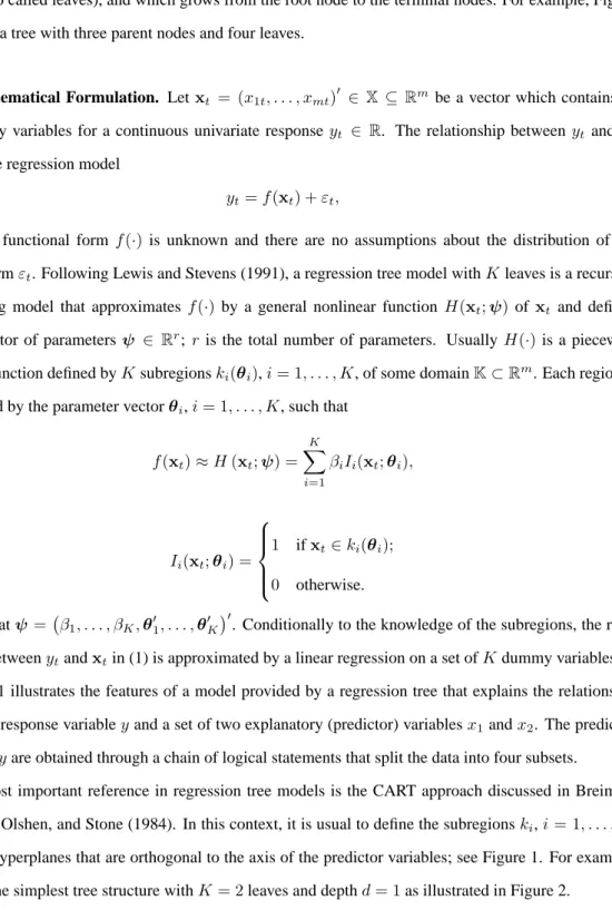
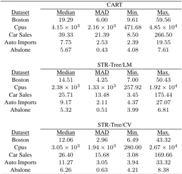
To get a honest picture of the performance reached by the specification algorithms, we conducted an out-of-sample evaluation by repeating 10 times a leave-10-out experiment. This resulted in a total of 100 out-of-sample squared errors. Table 7 reports the median, the MAD, the maximum, and the minimum of the squared errors over the 100 observations.
TABLE7. Out-of-Sample squared error of CART and STR-Tree Models based on 100 observations. CART
Dataset Median MAD Min. Max.
Boston 19.29 6.00 9.61 59.56 Cpus 4.15×10³ 2.16×10³ 471.68 4.85×10⁴ Car Sales 39.33 21.39 8.50 266.50 Auto Imports 7.75 2.53 2.39 19.55 Abalone 5.67 0.43 4.08 7.61 STR-Tree/LM
Dataset Median MAD Min. Max.
Boston 14.51 4.25 7.00 50.43 Cpus 2.38×10³ 1.33×10³ 257.92 1.92×10⁴ Car Sales 25.71 13.48 3.45 175.44 Auto Imports 9.17 2.11 4.37 27.07 Abalone 5.32 0.51 3.99 6.81 STR-Tree/CV
Dataset Median MAD Min. Max.
Boston 12.06 2.96 6.49 43.32 Cpus 3.05×10³ 1.94×10³ 280.00 2.67×10⁴ Car Sales 26.40 15.68 3.08 169.66 Auto Imports 11.27 3.05 3.94 33.32
Abalone 6.26 0.63 4.21 8.38
With the exception of the Auto Imports dataset, the STR-Tree model behaved better than CART. The STR-Tree model specified by a sequence of LM tests outperformed the STR-Tree models specified with cross-validations in four out five datasets.
However, if the number of terminal nodes is to be used for creating a cost-complexity measure, in the same spirit as proposed by Breiman, Friedman, Olshen, and Stone (1984)), the STR-Tree/LM approach is more parsimonious than CART in three out five cases as can be seen in Table 8. The STR-Tree/CV approach generates smaller trees than the STR-Tree/LM in four out five cases. Table 8 reports the median, the MAD, the minimum, and the maximum of the number of terminal nodes over 100 cases.
Table 9 shows the median, the MAD, the minimum, and the maximum of the computational time (in seconds) to specify each model, over 100 cases. All the programs were coded in Matlab 6.5.1. In the CART case, we used a customized function called treefit from the Statistical Toolbox. All the computations were carried out in a Pentium IV, 2.8 GHz with 1 Gb of RAM. It can be observed by inspection of Table 9 that
TABLE8. Number of Terminal Nodes Specified by CART and STR-Tree models based on 100 observations.
CART
Dataset Median MAD Min. Max.
Boston 7 1 4 15 Cpus 5 1 2 11 Car Sales 3 0 1 4 Auto Imports 9 2 3 16 Abalone 11 1.5 7 16 STR-Tree/LM Dataset Median MAD Min. Max.
Boston 9 1 4 12 Cpus 7 1 4 10 Car Sales 2 0 2 4 Auto Imports 4 0 4 7 Abalone 8 1 4 12 STR-Tree/CV Dataset Median MAD Min. Max.
Boston 7 1 4 12
Cpus 3 0 3 9
Car Sales 2 0 2 3
Auto Imports 3 1 2 6
Abalone 2 0 2 10
the computational burden involved in the STR-Tree/CV approach is dramatically high. The STR-Tree/LM strategy seems to be a very competitive alternative to CART.
TABLE9. Time (in seconds) spent by CART and STR-Tree models based on 100 observations. CART
Dataset Median MAD Min. Max.
Boston 29.69 0.94 22.85 40.43 Cpus 7.31 0.22 6.65 11.97 Car Sales 5.44 0.39 4.61 40.81 Auto Imports 11.02 0.58 8.07 12.36 Abalone 61.72 1.27 42.11 68.45 STR-Tree/LM
Dataset Median MAD Min. Max.
Boston 38.73 9.48 6.78 145.61 Cpus 28.80 5.06 17.17 66.56 Car Sales 10.93 2.30 1.23 43.52 Auto Imports 26.63 9.49 7.36 65.95 Abalone 91.06 15.56 64.13 495.61 STR-Tree/CV
Dataset Median MAD Min. Max.
Boston 1.07×10³ 161 570.00 1.85×10³ Cpus 197.00 19.9 161.00 604.50 Car Sales 121.00 8.2 92.80 227.10 Auto Imports 393.30 92.2 231.90 824.50
8. CONCLUSIONS
In this paper, we proposed a new model combines aspects of CART (Classification and Regression Trees) and STR (Smooth Transition Regression). The model is called the Smooth Transition Regression Tree (STR-Tree) and the main idea relies on replacing the indicator function in the usual CART by a logistic function. The resulting model can be analyzed as a smooth transition regression with multiple regimes. A detailed analysis of the asymptotic properties of the parameter estimates was presented and a model building procedure, based on a sequence of Lagrange Multiplier (LM) tests of hypotheses, was developed. An alternative specification strategy based on a 10-fold cross-validation was also discussed and a Monte Carlo experiment was carried out to evaluate the performance of the proposed methodology in comparison with standard techniques. The STR-Tree model outperforms CART when the correct selection of the architecture of simulated trees is considered. Furthermore, the LM test seems to be a promising alternative to 10-fold cross-validation. In addition to that, the proposed estimation algorithm seems to work properly in small samples. When put into proof with real datasets, the STR-Tree model has a superior predictive ability than CART. Finally, our STR-Tree model can be used in a random forest framework (Breiman 2001).
REFERENCES
AHN, H. (1996): “Log-Gamma Regression Modeling Through Regression Trees,” Communications in Statistics – Theory and Meth-ods, 25, 295–311.
AMEMIYA, T. (1983): “Non-Linear Regression Models,” in Handbook of Econometrics, ed. by Z. Griliches,andM. D.Intriligator, vol. 1, pp. 333–389. Elsevier Science.
BENJAMINI, Y.,ANDY. HOCHBERG(1995): “Controlling the False Dicovery Rate - A practical and Powerful Approach to Multiple
Testing,” Journal of teh Royal Statistical Society – Series B, 57, 289–300.
(1997): “Multiple Hypotheses Testing with Weights,” Scandinavian Journal of Statistics, 24, 407–418.
BENJAMINI, Y.,ANDW. LIU(1999): “A Step-Down Multiple Hypothesis Testing Procedures that Controls the False Discovery Rate
Under Independence,” Journal of Statistical Inference and Planning, 82, 163–170.
BENJAMINI, Y.,ANDD. YEKUTIELI(2000): “On the Adaptive Control of the Discovery Fate in Multiple Testing with Independent
Statistics,” Journal of Educational and Behavioral Statistics, 25, 60–83.
(2001): “The Control of the False Discovery Rate in Multiple Testing Under Dependency,” Annals of Statistics, 29, 1165– 1188.
BREIMAN, L. (2001): “Random Forests,” Machine Learning, 45, 5–32.
BREIMAN, L., J. H. FRIEDMAN, R. A. OLSHEN, AND C. J. STONE (1984): Classification and Regression Trees. Belmont
Wadsworth Int. Group, New York.
CIAMPI, A. (1991): “Generalized Regression Trees,” Computational Statistics and Data Analysis, 12, 57–78.
CROWLEY, J.,ANDM. L. BLANC(1993): “Survival Trees by Goodness of Split,” Journal of the American Statistical Association,
88, 457–467.
DAVIES, R. B. (1977): “Hypothesis Testing When the Nuisance Parameter in Present Only Under the Alternative,” Biometrika, 64, 247–254.
(1987): “Hypothesis Testing When the Nuisance Parameter in Present Only Under the Alternative,” Biometrika, 74, 33–44. DENISON, T., B. K. MALLIK,ANDA. F. M. SMITH(1998): “A Bayesian CART Algorithm,” Biometrika, 85, 363–377.
EITRHEIM, Ø., ANDT. TERASVIRTA¨ (1996): “Testing the Adequacy of Smooth Transition Autoregressive Models,” Journal of
Econometrics, 74, 59–75.
GRANGER, C. W. J.,ANDT. TERASVIRTA¨ (1993): Modelling Nonlinear Economic Relationships. Oxford University Press, Oxford.
HOCHBERG, Y. (1988): “A Sharper Bonferroni Procedure for Multiple Tests of Significance,” Biomatrika, 75, 800–802.
HORNIK, K., M. STINCHOMBE,ANDH. WHITE(1989): “Multi-Layer Feedforward Networks are Universal Approximators,” Neural
Networks, 2, 359–366.
JAJUGA, K. (1986): “Linear Fuzzy Regression,” Fuzzy Sets and Systems, 20, 343–353.
JENNRICH, R. I. (1969): “Asymptotic Properties of Non-linear Least Squares Estimators,” The Annals of Mathematical Statistics, 40, 633–643.
LEWIS, P. A. W., ANDJ. G. STEVENS(1991): “Nonlinear Modeling of Time Series Using Multivariate Adaptive Regression
Splines,” Journal of the American Statistical Association, 86, 864–877.
LUUKKONEN, R., P. SAIKKONEN, ANDT. TERASVIRTA¨ (1988): “Testing Linearity Against Smooth Transition Autoregressive
Models,” Biometrika, 75, 491–499.
MALINVAUD, E. (1970): “The Consistency of Nonlinear Regressions,” The Annals of Mathematical Statistics, 41, 956–969. MEDEIROS, M. C., T. TERASVIRTA¨ ,ANDG. RECH(2002): “Building Neural Network Models for Time Series: A Statistical
Approach,” Working Paper Series in Economics and Finance 508, Stockholm School of Economics.
MORGAN, J.,ANDJ. SONQUIST(1963): “Problems in The Analysis of Survey Data and a Proposal,” Journal of the American
Statistical Association, 58, 415–434.
P ¨OTSCHER, B. M.,ANDI. R. PRUCHA(1986): “A Class of Partially Adaptive One-step M-Estimators for the Non-linear Regression Model with Dependent Observations,” Journal of Econometrics, 32, 219–251.
SEGAL, M. R. (1992): “Tree-Structured Methods for Longitudinal Data,” Journal of the American Statistical Association, 87, 407– 418.
SUAREZ´ , A.,ANDJ. F. LUTSKO(1989): “Tree-Structured Methods for Longitudinal Data,” IEEE Transactions on Pattern Analysis
and Machine Intelligence, 21, 1297–1311.
TERASVIRTA¨ , T. (1994): “Specification, Estimation, and Evaluation of Smooth Transition Autoregressive Models,” Journal of the American Statistical Association, 89, 208–218.
(1998): “Modelling Economic Relationships with Smooth Transition Regressions,” in Handbook of Applied Economic Sta-tistics, ed. by A. Ullah,andD. E. A. Giles, pp. 507–552. Dekker.
VANDIJK, D.,ANDP. H. FRANSES(1999): “Modelling Multiple Regimes in the Business Cycle,” Macroeconomic Dynamics, 3(3), 311–340.
VANDIJK, D., T. TERASVIRTA¨ ,ANDP. H. FRANSES(2002): “Smooth Transition Autoregressive Models - A Survey of Recent Developments,” Econometric Reviews, 21, 1–47.
VENABLES, W. N.,ANDB. D. RIPLEY(2002): Modern Applied Statistics with S. Springer, New York.
WHITE, H. (1982): “Maximum Likelihood Estimation of Misspecified Models,” Econometrica, 50(1), 1–25. (1994): Estimation, Inference and Specification Analysis. Cambridge University Press, New York, NY.
WHITE, H.,ANDI. DOMOWITZ(1984): “Nonlinear Regression with Dependent Observations,” Econometrica, 52, 143–162.
WOOLDRIDGE, J. M. (1991): “On the application of robust, regression-based diagnostics to models of conditional means and condi-tional variances,” Journal of Econometrics, 47, 5–46.
(1994): “Estimation and Inference for Dependent Process,” in Handbook of Econometrics, ed. by R. F. Engle,andD. L. McFadden, vol. 4, pp. 2639–2738. Elsevier Science.
ZADEH, L. (1965): “Fuzzy Sets,” Information and Control, 8, 338–353.
Appendix A. PROOFS
Appendix A.1. Proof of Theorem 1. Lemma 2 of Jennrich (1969) shows that the conditions (1)–(3) in Theorem 1 are enough to guarantee the existence (and measurability) of the LSE (or the MLE in our case). In order to apply this result to the STR-Tree model we have to check if the above conditions are satisfied.
Condition (3) in Theorem 1 is satisfied by assumption; see Assumption 2. It is easy to prove in our case that
H(xt;ψ)is continuous in the parameter vectorψ. This follows from the fact that, for each value ofxt,Bk(xt;θk)in
(10) depend continuously onθk,k= 1, . . . , K. Similarly, we can see thatH(xt,ψ)is continuous inxt, and therefore
measurable, for each fixed value of the parameter vectorψ. Thus (1) and (2) are satisfied.
Q.E.D
Appendix A.2. Proof of Theorem 2. Following Jennrich (1969) and Amemiya (1983),ψ a.s.→ ψ∗if the following conditions hold:
(1) The parameter spaceΨis compact.
(2) QT(ψ)is continuous inψ∈ Ψfor allxt ∈ Xand for allyt ∈ R. FurthermoreQT(ψ)is a measurable
function ofxtandytfor allψ∈Ψ.
(3) plim
T→∞
T−1Q
T(ψ)exists, is non-stochastic, and converges uniformly inψ.
Condition (1) is satisfied by assumption; see Assumption 3. Using the results of Theorem 2, Condition (2) is trivially satisfied.
In order to check if Condition (3) is satisfied we will follow the steps presented in Amemiya (1983). From (10) and (11) we get 1 TQT(ψ) = 1 T T X t=1 ε2t+ 2 T T X t=1 [H(xt;ψ∗)−H(xt;ψ)]εt+ 1 T T X t=1 [H(xt;ψ∗)−H(xt;ψ)]2 ≡A1+A2+A3. (A.1)