Assessing Credit with Equity: A CEV
Model with Jump to Default
Luciano Campi
∗, Simon Polbennikov
†, and Alessandro Sbuelz
‡First version: November, 2004. This version: September 2005.
∗CEREMADE, Université Paris Dauphine, Place du Maréchal de Lattre de Tassigny,
75775, Paris Cedex 16, Phone: +33 (0) 1 44 05 4882, Fax: +33 (0)1 44-05-45-99, E-mail: [email protected].
†Econometrics and Operations Research, Tilburg University, The Netherlands, Phone:
+31-13-4663426, E-mail: [email protected].
‡Corresponding author. Department of Economics, SAFE Center, University of
Verona, Via Giardino Giusti 2, 37129, Verona, Italy, Phone: +39-045-8054922 , Fax: +39-045-8054935 , E-mail: [email protected].
Assessing Credit with Equity: A CEV Model with Jump to Default
Abstract
Unlike in structural and reduced-form models, we use equity as a liquid and observable primitive to analytically value corporate bonds and credit default swaps. Restrictive assumptions on the firm’s capital structure are avoided. Default is parsimoniously represented by equity value hitting the zero barrier. Default can be either predictable, according to a CEV process that yields a positive probability of diffusive default and enables the leverage effect, or unpredictable, according to a Poisson-process jump that implies non-zero credit spreads for short maturities. Easy cross-asset hedging is enabled. By means of a carefully specified pricing kernel, we also enable an-alytical credit-risk management under possibly systematic jump-to-default risk.
JEL-Classification: G12, G33.
Keywords: Equity, Corporate Bonds, Credit Default Swaps, Constant-Elasticity-of-Variance (CEV) Diffusion, Jump to Default.
1
Introduction
For individualfirms in segments of the market with high default risk there is a clear link between default risk and equity returns and default risk ap-pears to be systematic (Vassalou and Xing (2004)). Investors and credit-risk managers seem to have taken notice. Investors have been showing appetite for models that simultaneously handle credit and equity instruments, which is important in managing a portfolio of these two instruments. Indeed, cross-asset trading of credit risk has been gaining momentum1 among hedge funds and banks. In their effort of assessing objective probabilities of de-fault, credit-risk managers have been courting credit-risk models that focus on equity data2 and that, given the systematic nature of default risk, could explicitly treat the relationship between the objective probability measure and the pricing measure(s).
Reduced-form models (see for example Duffie (1999) and the excellent reviews in Lando (2004) and Schönbucher (2003)) are not of great help, as they miss the direct linkage to the firm’s capital structure. Structural models are driven by the value evolution infirm’s assets. The assets-value evolution is often assumed to be diffusive so that the default can be seen predictably coming by observing changes in the capital structure of thefirm (see the seminal papers of Merton (1974) and Black and Cox (1976) and the reviews in Lando (2004) and Schönbucher (2003)). While appealing,
1
The rise of capital structure arbitrage is a good example (see Yu (2004)).
2
KMV output is strongly driven by equity-value data. The observation that, for non-investment-grade reference entities, prices in credit default swap, corporate bond, and equity markets tend to adjust simultaneously (see Schaefer and Strebulaev (2003) and D’Ecclesia and Tompkins (2005)) impacts credit-risk management by affecting the assess-ment of the objective probability of default (see D’Ecclesia and Tompkins (2005)).
structural models suffer when it comes to applications. The underlying (the sum offirm’s liabilities and equity) is illiquid and often non-tradable. Obtaining accurate asset volatility forecasts and reliable capital structure leverage data is difficult. Predictability of the default event implies the counterfactual prediction of zero credit spreads for short maturities3 and, last but not least, arbitrary use of the structural default barrier is often a temptation hard to resist−endogenous barriers4 are impractical because of the capital-structure assumptions under which they are derived are not fully realistic.
We propose a parsimonious credit risk model that does look at thefirm’s balance sheet but avoids the application mishaps of structural models. We take as underlying the most liquid and observable corporate security: Eq-uity. This modelling choice brings in hedging viability and the possibil-ity of reliable model calibration-leverage information from book values can be circumvented. We parsimoniously represent default as equity value hit-ting the zero barrier either diffusively or with a jump. The presence of an equity-value drop to zero has its credit-risk foundation in the incom-pleteness of accounting information (see Duffie and Lando (2001)), rules out default predictability, and embeds the concept of unexpected default, typical of reduced-form models, within a credit-risk model that is directly based on equity. We assume that the continuous-path part of equity value is a Constant-Elasticity-of-Variance (CEV) diffusion5, which enables a
pos-3Zhou (1997) posits assets-value jumps to overcome default predictability. Duffie and
Singleton (2001) explain such jumps with the presence of incomplete accounting informa-tion.
4See for example Leland and Toft (1996), Acharya and Carpenter (2002), and references
therein.
itive probability of absorption at zero andfits the stylized fact of a negative link between equity volatility and equity price (the so-called ‘leverage ef-fect’), and that the jump to default is driven by an independent Poisson process. Such distributional assumptions prompt us to obtain closed forms for Corporate Bond (CB) prices and Credit Default Swap (CDS) fees, from which hedge ratios can be easily calculated. Those assumptions and a care-ful specification of the state-price density also empower analytical credit-risk management−we provide a closed form for the objective default probabilities in the presence of possibly systematic jump-to-default risk.
Albanese and Chen (2004) and Campi and Sbuelz (2004) also use a CEV-equity model to price credit instruments but they disregard the default pre-dictability issue. In deriving closed-form values, we build upon a CEV result in Campi and Sbuelz (2004). Brigo and Tarenghi (2004), Naik, Trinh, Bal-akrishnan, and Sen (2003) and Trinh (2004) introduce a hybrid debt-equity model that considers equity as primitive but that, like structural models, necessitates a free default barrier, which is then left to potentially ad-hoc
uses−equity value is assumed to be a geometric Brownian motion, except in Brigo and Tarenghi (2004)6. Das and Sundaram (2003) have proposed an equity-based model that accounts for default risk, interest risk, and equity risk using a lattice framework. As such, they do not seek hedger-friendly analytical solutions. Numerical credit risk pricing based on equity has also the CEV-based asset-pricing literature includes the works of Albanese, Campolieti, Carr, and Lipton (2001), Beckers (1980), Boyle and Tian (1999), Cox and Ross (1976), Davydov and Linetsky (2001), Emanuel and MacBeth (1982), Forde (2005), Goldenberg (1991), Leung and Kwok (2005), Lo, Hui, Yuen (2000), Lo, Hui, and Yuen (2001), Lo, Tang, Ku, and Hui (2004), Sbuelz (2004), and Schroder (1989).
6Brigo and Tarenghi (2004) and Hui, Lo, and Tsang (2003) employ a flexible
been suggested by the convertible bond7 literature (see, for example, An-dersen and Andreasen (2000), AnAn-dersen and Buffum (2003), and Tsiveriotis and Fernandes (1998); McConnell and Schwartz (1986) ignore the possibil-ity of bankruptcy). In Cathcart and El-Jahel (2003), default occurs when a geometric-Brownian-motion signaling variable, interpreted as the credit quality of the reference entity, hits a lower default barrier or according to a hazard rate process, so that both expected and unexpected defaults are accomodated in a single framework. However, the signaling variable can hardly be identified with equity value (the default barrier is above the in-accessible zero level and there is no ‘leverage effect’) and the problem of a possibly freewheeling default barrier remains.
Linetsky (2005) builds upon the convertible bond literature to assess zero-coupon CB prices within a geometric-Brownian-motion model with jump-like bankruptcy where the hazard rate of bankruptcy is a negative power of the share price. The dependence of the hazard rate on the share price strongly complicates the analysis8. In a recent independent work, Carr and Linetsky (2005) take the stock price to follow a CEV diffusion, punc-tuated by a possible jump to zero. To capture the possible positive link between default and volatility, they assume that the hazard rate of default is an increasing affine function of the instantaneous variance of returns on the underlying stock. Carr and Linetsky (2005) pursue a risk-neutral pricing analysis without showing the existence of some equivalent martingale mea-sure in their incomplete-markets setting−with CEV-like complete markets,
7
See Nelken (2000) for a review of hybrid debt-equity instruments.
8
The valuation formulae in Linetsky (2005) are spectral expansions that embed sin-gle integrals with respect to the spectral parameter and calculations imply the use of numerical-integration routines.
Delbaen and Shirakawa (2002) show existence for a given lower bound on the CEV parameter. Also, no study of the pricing-kernel-based choice of an equivalent martingale measure is attempted.
By contrast, the (possibly) systematic nature of CEV-like diffusive risk as well as of jump-to-default risk is carefully and parsimoniously treated in our work. In particular, we prove that our parametric pricing kernel9 does support equivalent martingale measures. In doing so, we extend the existence result of Delbaen and Shirakawa (2002) to any negative value of the CEV parameter.
The rest of the work is organized as follows. Section 2 describes the un-derlying equity value process. Section 3 provides analytical results for CBs and CDSs. Section 4 specifies a pricing kernel that permits analytical ob-jective default probabilities. After the conclusions (Section 5), an Appendix gathers lengthy proofs, analytical formulae, and details about model-based hedging.
9Since the jump to default is not a stopping time of thefiltration generated by the
continuous-path part of the stock price, our chosen Radon-Nikodym derivative is simi-lar to the one coming from dynamic asset pricing theory with uncertain time-horizon, Blanchet-Scaillet, El Karoui, and Martellini (2005), Proposition 2. Bellamy and Jean-bleanc (2000) analyze the incompleteness of markets driven by a mixed diffusion, construct a similar Radon-Nikodym derivative, and, among other contingent claims, study Ameri-can contracts. Both Blanchet-Scaillet, El Karoui, and Martellini (2005) and Bellamy and Jeanbleanc (2000) assume bounded local volatility for the stock returns, which is not our CEV case. They also refrain from considering default-driven time-horizon uncertainty.
2
The equity value
Under an equivalent martingale measure10 Q, the reference entity’s share-price process{S} has the following pre-default jump-diffusion dynamics:
dSt
St−
= (r−q)dt+σStρ−−1dzt−(dNt−λdt).
Here below we list the main objects appearing in the dynamics of{S}: (i) S0=S (current share price),
(ii) St−≡limε&0St−ε (left time limit),
(iii) ρ−1<0 (constant elasticity of the diffusive volatility), (iv) Nt≥0(first-jump-stopped Poisson process),
(v) τ ≡inf{t:Nt= 1} (time of jump-like default),
(vi) E0Q£1{τ >T}
¤
= exp (−λT) (chance of surviving to jump-like default), (vii) T >0 (finite maturity, in years),
(viii) λ≥0 (jump-to-default intensity),
where r is the constant riskfree rate, q is the constant dividend yield11,
σ (σ >0) is a constant scale factor for the diffusive volatility, anddz is the increment of a Wiener process under Q. The processes {z} and {N} are
1 0Given our incomplete-markets setting, see Section 4 for a discussion of a tractable
relationship between admissibleQs and the objective measureP.
1 1We consider the caser
assumed to be independent. The assumed absence of interest rate risk is unlikely to be restrictive for non-investment-grade reference entities, as the interest-rate sensitivity of credit instruments (mainly CBs) related to those entities is low (see Cornell and Green (1991) and Guha and Sbuelz (2003)). According to the boundary classification, an inverse relationship between volatility and share price(ρ−1<0)is necessary to have absorption at zero with positive probability mass in the absence of jumps. Such an assump-tion of inverse relaassump-tionship not only enables predictable default at the zero barrier, but it is also consistent with much empirical evidence on the nega-tive correlation between stock returns and their volatilities. Realized stock volatility is negatively related to stock price. This ‘leverage effect’ wasfirst discussed in Black (1976) and its various patterns have been documented by many empirical studies, for example, Christie (1982), Nelson (1991), and Engle and Lee (1993).
The time of absorption at zero in the absence of jumps isξ, that is
ξ ≡ inf{t:St= 0, Nt= 0},
whereas the time of absorption at zero tout court is the minimum between
τ and ξ, that is
We take the point0to be the absorbing state of the share-price process{S}, so that, once default has occurred, the share price remains at zero,
St = 0, ∀t≥τ ∧ξ.
We also introduce the time of absorption at zero of the continuous part{Sc}
of{S}, that is, ξc ≡ inf{t:Stc= 0}, where dSc t Stc = (r−q+λ)dt+σ(S c t)ρ−1dzt,
so thatξc and τ are clearly independent.
3
Analytical results for CBs and CDSs
Let T > 0 be a finite maturity (in years) and let VQ(S, T, y) be the T -truncated Laplace transform ofτ∧ξ’s probability density function underQ (Q-p.d.f.) with Laplace parametery (y≥0),
Such a quantity is of great importance, as it is the building block for the an-alytical pricing of CBs and CDSs (with maturityT). VQ(S, T, r)represents the fair present value of 1 unit of currency at the reference entity’s default if default occurs withinT, while VQ(S, T,0)represents the risk-neutral prob-ability of default withinT.
The next proposition is a neat and useful result stemming from the in-dependence between{z}and{N}. It gives an analytical characterization of
VQ(S, T, y). It states that the quantity of interest is the linear convex com-bination of the adjusted risk-neutral probability of default within T (with weight y+λλ) and of the(y+λ)-discounted value of 1 unit of currency at the diffusive default within T (with weight y+yλ). The latter is theT-truncated Laplace transform ofξc’sQ-p.d.f. with Laplace parametery+λ,
E0Q£exp (−(y+λ)ξc)1{ξc ≤T}
¤
,
and its closed form12has been recently derived by Campi and Sbuelz (2004). The closed form is provided in the Appendix.
Proposition 1 Under the above assumptions, theT-truncated Laplace trans-1 2Davidov and Linetsky (2001), see pp. 953 and 956, point out that theT-truncated
Laplace transform of ξc’s Q-p.d.f. with Laplace parameter y+λ can be obtained by numerically inverting the closed-form non-truncated Laplace transform
1 aE Q 0 [exp (−(y+λ+a)ξ c )], where the inversion parameter isa >0.
form ofτ ∧ξ’sQ-p.d.f. with Laplace parametery is VQ(S, T, y) = λ y+λ h 1−exp (−(y+λ)T)³1−E0Q£1{ξc ≤T} ¤´i + y y+λE Q 0 £ exp (−(y+λ)ξc)1{ξc ≤T} ¤ .
Proof. See the Appendix.
Proposition 1 empowers analytical pricing of CBs and CDSs. Consider a reference entity’s CB that has face valueF and pays an (annualized) coupon
Cat regular 1k-spaced datesTj up to its maturityT (kis a positive integer).
For the sake of simplifying notation, we take the maturityT to be a rational number of the type nk,n∈N.
Proposition 2 Given the recovery rateR at default and given the assump-tion of Recovery of Face Value at Default (RFV), the fair CB price is
PCB(S, T, r) = kT X j=1 1 kexp (−rTj) h 1−VQ(S, Tj,0) i C + exp (−rT)h1−VQ(S, T,0)iF +VQ(S, T, r)·R·F.
Proof. The result comes from taking the Q-expectation of CB’s dis-counted payoffs. RFV bears the valueVQ(S, T, r)·R·F for CB’s defaultable part.
Ris afixed historical data input in applications. Under RFV, CB holders receive the same fractional recovery R of the face value F at default for CBs issued by the reference entity regardless of maturity. Guha and Sbuelz (2003) show that the RFV recovery form is consistent with typical bond indenture language (for example, the claim acceleration clause), defaulted bond price data, and relevant stylized facts of non-defaulted bond price data (the mentioned low duration of high-yield bonds; see Cornell and Green (1991)).
Consider a CDS related to the CB just described. It offers a protection payment of (1−R)F in exchange for an (annualized) fee fCDS paid at
regular 1k-spaced dates up to the contract’s maturity. Proposition 3 The fair CDS fee is
fCDS(S, T, r) =
VQ(S, T, r) (1−R)
PkT
j=1k1exp (−rTj) [1−VQ(S, Tj,0)]
.
Proof. Under Q, the fee fCDS(S, T, r) zeroes the CDS’ net present
value.
The holder of a CB can achieve total recouping of the face valueF at de-fault by being long a CDS. Being short ∂S∂ PCB(S, T, r)shares Delta-hedges13 1 3We already remarked that interest-rate sensitivity of bonds issued by
non-high-credit-quality entities is low. However, parallel shifts of the (flat) term structure of the interest rates can be hedged by selling a portfolio of default-free bonds that has interest-rate
against the pre-default price shocks driven by diffusive news. Recent evi-dence shows that such equity-based hedges perform reasonably well for high-yield CBs (see Naik, Trinh, Balakrishnan, and Sen (2003) and Schaefer and Strebulaev (2003)). Given analytical CB prices, an easy and effective mea-sure of the Delta-hedge ratio is
∂
∂SPCB(S, T, r) '
PCB(S+ε, T, r)−PCB(S−ε, T, r)
2ε ,
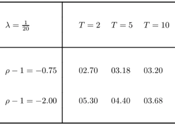
for a smallε. More details on model-based CB hedging are in the Appendix. Tables 1 and 2 exhibit, across different maturities and levels of the pa-rameterρ, the yield spread of a semiannual-coupon 7% CB and the fee of a CDS with quarterly installments. The left-hand (right-hand) panel fixes
λ = 201 (λ = 101), that is, it refers to a situation in which, on Q-average, there is one chance of jump-like default every 20 (10) years. Positive levels of the the risk-neutral jump intensity exert the remarkable pricing impact (for short maturities in particular) that is known from pure reduced-form models. The ‘leverage effect’ is quite important in boosting CB spreads and CDS fees, especially at low levels of the risk-neutral jump intensity.
Table 1: The CB spread (promised yield to maturity minus r, %) The input values areC= 7%,F= $100, R= 50%, S= $1,k= 2,r= 5%,q= 2%, and
σ= 35%. sensitivity equal to ∂
∂rPCB(S, T, r). Such a hedge ratio can be easily calculated in our
model as PCB(S,T,r+ε)−PCB(S,T ,r−ε)
λ=201 T = 2 T = 5 T = 10 λ= 1
10 T= 2 T = 5 T = 10
ρ−1 =−0.75 02.70 03.18 03.20 05.05 05.13 04.79
ρ−1 =−2.00 05.30 04.40 03.68 07.06 05.97 05.14
Table 2: The CDS fee (%)
The input values areR= 50%, S= $1,k= 4,r= 5%,q= 2%, andσ= 35%.
λ=201 T =12 T= 2 T = 5 λ=101 T =12 T = 2 T= 5
ρ−1 =−0.75 02.53 02.71 03.25 05.09 05.22 05.57
ρ−1 =−2.00 03.88 05.48 04.74 06.28 07.49 06.78
4
The objective default probability
Our equity-based model contributes also to credit risk management by being conducive to closed forms for the objective default probability14,V P(S, T,0),
1 4
For example, the New Basel Capital Accord allows the use of model-based objective probabilities of default to determine the appropriate level of reserves to support credit risky activities.
with
VP(S, T, y) ≡ E0Phexp (−y(τ ∧ξ)){τ∧ξ≤T}i,
where P is the objective probability measure. A parsimonious and closed-form-conducive way of specifying the dynamics of the share price process
{S}under the objective measure is the following:
dSt St− = µPdt+σStρ−−1dztP− ³ dNtP−λPdt ´ , where (i) µP ≡r−q+θσ+EP[(exp(ζ)−1)]λ P,
(ii) θσ≥0 (premium for the diffusive risk),
(iii) EP[(exp(ζ)−1)]λP ≥0 (premium for the jump-like default risk).
ζ is a random variable independent from {zP} and {NP}, which are assumed to be independent15. Such a terse specification of{S}’sP-dynamics makes a neat account of systematic jump-like default risk. The risk-neutral
1 5
jump-to-default intensity λ maintains a simple link to the objective jump-to-default intensity λP (λP>0):
λ = EP[exp (ζ)]λP.
If the jump-like default risk disappears (λP & 0 ), its premium shrinks to zero and the risk-neutral jump-to-default intensity does so as well. In the case of a jump to default (τ ∧ξ = τ), the state-price-density process {π}
that backs the measureQjumps fromπτ− toπτ,
πτ = πτ−exp (ζ).
Sinceπτ provides the fair present value of 1 unit of currency received at the
time of jump-like default per unit probability of such a dislikeable event, it is reasonable to impose the restriction that πτ must always be at least
as much as πτ− is. Such restriction is granted by a non-negative ζ, which
forces the risk premium EP[(exp(ζ)−1)]λP to be non-negative. This is in line with the finding of Vassalou and Xing (2004) that high default risk firms earn higher equity returns than low default risk firms. The criterion of parameter parsimony suggests to take forζ a one-parameter non-negative distribution. One such distribution is the discrete Poisson distribution with parameterφ (φ >0) and with support {0,1,2, ...}, so that the expectation
EP[exp (ζ)] admits a concise closed form,
EP[exp (ζ)] = exp (φ(e−1))>1,
EP[ζ] = φ,
V arP[ζ] = φ.
As long as jump-like default risk is systematic (φis well above0), the jump-to-default intensity underQis always greater than its level underP(λ > λP). If the state-price density does not jump in the case of a jump to default (φ&0, that is,ζ = 0P-almost surely), the systematic nature of the jump-like default risk is washed away so that risk-neutral and objective jump-to-default intensities tend to coincide (λ&λP).
As far as diffusive risk is concerned, if its premium faints, it is either because such a risk is not priced (θ & 0) or because the risk is dimming (σ &0).
The above specification of{S}’s P-dynamics forces{π}’s P-dynamics to be as follows.
process{π} is dπt πt− = −rdt −θSt1−−ρdzPt + ³ (exp (ζ)−1)dNtP−[exp (φ(e−1))−1]λPdt ´ , and, for t ≥τ ∧ξ, πt = πτ∧ξexp (−r(t−τ ∧ξ)).
Proof. If the process {π} has the stated P-dynamics, then there are no arbitrage opportunities. By virtue of Itô’s Formula, theπ-deflated gain processes generated by holding one share and by holding one unit of currency in the money-market account are localP-martingales,
EtP[d(πt·Stexp (qt))] = 0, EtP[d(πt·exp (rt))] = 0,
and, hence, the market is arbitrage-free16.
1 6
This indeed rules out arbitrage opportunities involvingStexp (qt)andexp (rt), under
natural conditions on dynamic trading strategies. See, for example, Appendix B.2 in Pan (2000).
We can even say more. Given finite values for θ and φ, our chosen state-price-density process does support an equivalent martingale measure
Q.
Proposition 5 Let πt be defined as above and letT >0 be any finite time horizon. Then, the local P-martingale process {ertπ
t}, is a P-martingale over [0, T].
Proof. See the Appendix.
The previous proposition can be rephrased as follows: since the π -deflated gain process generated by holding one unit of currency in the money-market account is also a P-martingale, its T-time level represents the Radon-Nikodym derivative ofQwith respect toP ,πTexp(rT) = ddQP.
Given our choice of the pricing kernel, the quantity VP(S, T, y) admits an analytical expression and, as soon as diffusive risk and/or jump-to-default risk are systematic, it is always smaller than the quantityVQ(S, T, y)for any
y. In particular, systematic risk makes the P-probability of default smaller than theQ-probability of default.
Proposition 6 The quantity VP(S, T, y) has the following closed form:
VP(S, T, y) = λP y+λP h 1−exp (−(y+λP)T)³1−E0P£1{ξc ≤T} ¤´i + y y+λPE P 0 £ exp (−(y+λP)ξc)1{ξc ≤T} ¤ ,
TheT-truncated Laplace transform ofξc’sP-p.d.f. with Laplace param-eter y+λP is analytical (see Campi and Sbuelz (2004)). Its closed form is provided in the Appendix.
Table 3 exhibits, across different maturities and levels of the parameter
ρ, the probabilities of default VQ(S, T,0)and VP(S, T,0). The equity
pre-mium isfixed atµP−(r−q) = 12%by choosing a pricing kernel that, given
λ= 101, implies on average one chance of jump-like default every16.67years under the objective probability measureP(λP = 161.67). A greater ‘leverage effect’ clearly inflates the probabilities of default, which, even if the drifts
r−q and µP+λP are positive, remain non-defective (they approach 1 as
T goes to infinity) under both Q and P as long as jump-like default has a non-zero chance to occur (λand λP are positive).
Table 3: The probability of default under Q and P (%) The input values areS= $1,r= 5%,q= 2%,σ= 35%,λ=101, andθandφsuch that the risk premiaθσand[exp (φ(e−1))−1]λP are8%and4%, respectively. This implies
thatµP= 15%andλP=16.671 . VQ(S, T,0) T =1 2 T= 2 T = 5 VP(S, T,0) T = 1 2 T = 2 T = 5 ρ−1 =−0.75 04.88 18.56 42.51 02.96 11.58 27.89 ρ−1 =−2.00 05.97 25.45 47.51 03.85 16.87 32.05
In summary, we achieve analytical objective probabilities of default by augmenting the original parameter set {r, q, σ, ρ, λ} with two risk-pricing parameters only,θfor the diffusive risk andφfor the jump-like default risk.
5
Conclusions
We present an equity-based credit risk model that, by taking as primitive the most liquid and observable part of afirm’s capital structure, overcomes many of the problems suffered by structural models in pricing and hedging applications. Our parsimonious model avoids any assumption on the firm’s liabilities. It empowers the analytical pricing of CBs and CDSs and it can match non-zero short-maturity spreads. Cross-asset hedging is viable and easy to implement. A careful specification of the state price density enables analytical credit-risk management in the presence of systematic jump-to-default risk.
6
Appendix
Proof of Proposition 1 We have that E0Q£{τ∧ξ>s}¤ = E0Q£1{τ >s}1{ξ>s}¤ = E0Q[1{τ >s}E0Q£1{ξ>s}|Nu= 0, u≤s ¤ ] = E0Q[1{τ >s}E0Q£1{ξc>s }|Nu = 0, u≤s ¤ ] = E0Q£1{τ >s}¤E0Q£1{ξc>s } ¤ ,where the last equality follows from the independence between ξc and τ. Hence, the time-s-evaluated Q-p.d.f. of the stopping timeτ ∧ξ is
fτ∧ξ(s) = − d dsE Q 0 £ 1{τ∧ξ>s} ¤ = −d ds ³ E0Q£1{τ >s}¤E0Q£1{ξc>s } ¤´ = fτ(s)E0Q £ 1{ξc>s}¤+fξc(s)EQ 0 £ 1{τ >s} ¤ = λexp (−λs)EQ0 £1{ξc>s } ¤ +fξc(s) exp (−λs).
parametery is VQ(S, T, y) = EQ0 £exp (−y(τ∧ξ))1{τ∧ξ≤T}¤ = Z T 0 exp (−ys)fτ∧ξc(s)ds = λY1+Y2, Y1 = Z T 0 exp (−(y+λ)s)E0Q£1{ξc>s}¤ds, Y2 = Z T 0 exp (−(y+λ)s)fξc(s)ds.
Y2 is the T-truncated Laplace transform of ξc’s Q-p.d.f. with Laplace pa-rametery+λ, Y2=EQ0 £ exp (−(y+λ)ξc)1{ξc ≤T} ¤ .
Its closed form has been derived by Campi and Sbuelz (2004) and it can be found below after this proof. An integration by parts gives
Y1 = − 1 y+λexp (−(y+λ)s)E Q 0 £ 1{ξc>s } ¤¯¯¯ ¯ T 0 − Z T 0 −1 y+λexp (−(y+λ)s) ¡ −fξc(s)¢ds = 1 y+λ h 1−exp (−(y+λ)T)E0Q£1{ξc>T } ¤i −y+1 λY2.
Proof of Proposition 5 We will use the following auxiliary result:
Lemma 7 Let ρ <1, so possibly taking negative values, Sc be the continu-ous part of S as previously defined and let ηt be defined as follows:
ηt≡E µ −θ Z · 0 (Suc)ρ−1dzuP ¶ t , t≥0.
Then, for any 0 < T < ∞, {η} is a true P-martingale over [0, T]. In particular, E0P[ηT] = 1.
Proof. Following the proof of Theorem 2.3 in Delbaen and Shirakawa (2002), the crucial argument for ηt to be a true P-martingale is that the integral R0T(Suc)2(1−ρ)du is finite a.s.. Delbaen and Shirakawa (2002) show that this is the case forρ∈(0,1). We notice that the integralR0T(Suc)2(1−ρ)du
remainsfinite a.s. even forρ≤0. Indeed,Sc has continuous trajectories so that the integral cannot explode.
To simplify the notation, we set eπt := ertπt. From the dynamics of πt
follows that
deπt=eπt−[−θS1t−−ρdztP+ ((eζ−1)dNtP−EP0[eζ−1]λP)dt], t < τ ∧ξ
and eπt =eπτ∧ξ fort≥ τ∧ξ. The initial condition is of course π0e = 1. We
can write the processeπtas a Doléans-Dade stochastic exponential (see, e.g.,
Protter (1990), p. 78) in the following way: e πt=E µ − Z · 0 θSu1−−ρdzuP ¶ t∧τ∧ξ Yt∧τ∧ξ,
where we set Yt ≡ exp ½Z t 0 (eζ−1)dNuP− Z t 0 E0P[eζ−1]λPdu ¾ ×Y u≤t (1 + (eζ−1)∆NuP)e−(eζ−1)∆NuP = exp X u≤t ln (1 + (eζ−1)∆NuP)− Z t 0 E0P[eζ−1]λPdu . Fix a finite time horizonT >0. Wefirst prove that the process
E µ − Z · 0 θSu1−−ρdzuP ¶ t∧τ∧T Yt∧τ∧T, t≥0, (1)
is a P-martingale. To do so, we observe that, being (1) a strictly positive local P-martingale, it is a P-supermartingale too17. To show that it is a
P-martingale, it suffices to prove thatE0P[E(−R θSu1−−ρdzuP)τ∧TYτ∧T] = 118. 1 7This comes from the following well-known fact from martingale theory: let
M = (Mt)t≥0 be a local martingale defined on a given filtered probability space
(Ω,(Ft)t≥0,F, P)and bounded from below by a constanta >0, i.e. Mt≥ −afor eacht.
Then,M is a supermartingale. Indeed, letτnbe a localizing sequence of stopping times
forMt, i.e. τn↑+∞a.s. and every stopped process(Mt∧τn)t≥0 is a true martingale, for
eachn. Fix two instantss≤t. Fatou’s lemma gives E[Mt|Fs] =E[lim inf
n→∞ Mt∧τn|Fs]≤lim infn→∞ E[Mt∧τn|Fs] =Ms.
1 8
Indeed, let0< T <∞and let M = (Mt)t∈[0,T] be a supermartingale defined on a
givenfiltered probability space(Ω,(Ft)t∈[0,T],F, P)whereF0is trivial, such thatE[MT] =
M0. ThenM is a martingale. To prove this, observe that, sinceE[MT]≤E[Mt]≤M0for
eacht∈[0, T], the conditionE[MT] =M0 is equivalent toE[Mt] =M0 for allt∈[0, T].
This implies that
E[Ms−E[Mt|Fs]] =E[Ms]−E[Mt] = 0,
for every couple of instantss≤ t ≤T. Since the supermartingale property gives that Ms−E[Mt|Fs]≥0, we haveE[Mt|Fs] =Ms.
Indeed, note that, in the stochastic exponential, we can replace the process
S with its continuous part Sc, which is independent of NP and ζ by con-struction. Conditioning with respect toτ and ζ gives
E0P · E µ − Z · 0 θSu1−−ρdzPu ¶ τ∧T Yτ∧T ¸ = E0P · E0P · E µ − Z · 0 θ(Suc−)1−ρdzPu ¶ τ∧T |τ , ζ ¸ Yτ∧T ¸ = E0P " E0P · E µ − Z · 0 θ(Suc−)1−ρdzPu ¶ t ¸ |t=τ∧T Yτ∧T # = E0P[Yτ∧T].
Thefirst equality is due to the fact that
Yτ∧T = exp n ln³1 + (eζ−1)1{τ≤T} ´ −E0P[eζ−1]λP(τ∧T)o = (1 + (eζ−1)1{τ≤T})e−E P 0[eζ−1]λP(τ∧T),
so that it depends only on τ and ζ. The second equality follows from the independence of τ,ζ and Sc and the third one from Proposition 7, stating
in particular that E0P[E¡−R0·θ(Suc−)1−ρdzPu¢t
∧T] = 1.
It remains to computeEP
0[Yτ∧T]. To do so, recall thatτ is exponentially
distributed with parameter λP, so that P[τ > T] = e−λPT. Then, being ζ
and τ independent by assumption, we have
E0P[Yτ∧T] = E0P[eζe−E P 0[eζ−1]λPτ1 {τ≤T}] +EP0[e−E P 0[eζ−1]λPT1 {τ >T}] = E0P[eζ]E0P[e−E0P[eζ−1]λPτ1 {τ≤T}] +e−E P 0[eζ−1]λPTP[τ > T] = E0P[eζ] Z T 0 λPe−E0P[eζ]λPtdt+e−E0P[eζ]λPT = 1−e−E0P[eζ]λPT +e−E0P[eζ]λPT = 1.
This yields that E(−R θSu1−−ρdzuP)t∧τ∧TYt∧τ∧T is aP-martingale. Doob’s
optional sampling theorem applies (e.g., Theorem 18 in Protter (1990)) and gives that the processπetis aP-martingale over the time interval[0, T]. Being
The discounted value of cash at ξc within T
TheT-truncated Laplace transform ofξc’sQ-p.d.f. with Laplace param-eterw (w≥0) has been shown by Campi and Sbuelz (2004) to be
E0Q£exp (−w·ξc)1{ξc ≤T} ¤ = lim &0 ∞ X n=0 an(A, B) ³x 2 ´nΓ(ν−n, x 2K, x 2 ) Γ(ν) , where Γ(ν) ≡ Z +∞ 0 uν−1e−udu (Gamma Function), Γ³ν−n, x 2K, x 2 ´ ≡ Z x 2 x 2K
u−nuν−1e−udu (Generalized Incomplete Gamma Function),
an(A, B) ≡ (−1)nC(B, n)An, C(B, n) ≡ Qn k=1(B−(k−1)) n! 1{n≥1}+1{n=0}, x ≡ S2(1−ρ), ν ≡ 1 2(1−ρ), A ≡ 2 (r−q+λ) σ2(1−ρ) , K ≡ σ2(1−ρ) 2 (r−q+λ) ³ 1−e−2T(r−q+λ)(1−ρ)´, B ≡ w .
The Generalized Incomplete Gamma Function, the Incomplete Gamma Func-tion, and the Gamma function are built-in routines in many computing soft-ware like MATLAB and Mathematica, which makes the above expressions fully viable.
Model-based CB hedging
Full dynamic hedging of a long position in a CB implies being short η
units of stocks as well as being long ξ units of CDSs with given fee f (for recovery rateZ and notionalX), where η andξ are adapted processes that satisfy the following system of risk-nullifying equations:
0 = ∂ ∂SPCB − η+ξ ∂ ∂S VQ(S, T, r) (1−Z)X −PkTj=11kexp (−rTj) £ 1−VQ(S, Tj,0)¤f , 0 =R·F − PCB(S, T, r) −η(0−S) +ξ(1−Z)X −ξ VQ(S, T, r) (1−Z)X −PkTj=11kexp (−rTj) £ 1−VQ(S, Tj,0)¤f .
Our model also states that, in the case of a jump to default (τ∧ξ=τ), pure Delta hedging recoups a fraction
∂
∂SPCB(Sτ−, T −τ , r)Sτ−
PCB(Sτ−, T −τ , r)−R·F
The objective probability of default at ξc within T
The replacement of the risk-neutral intensity-added driftr−q+λwith the objective intensity-added drift µP +λP implies that the T-truncated Laplace transform of ξc’s P-p.d.f. with Laplace parameter w (w ≥ 0) has this analytical expression:
E0P£exp (−wξc)1{ξc≤T}¤ = lim &0 ∞ X n=0 an(AP, BP) ³x 2 ´nΓ(ν−n,2Kx P, x 2 ) Γ(ν) , for AP ≡ 2 (µP+λP) σ2(1−ρ) , KP ≡ σ 2(1 −ρ) 2 (µP+λP) ³ 1−e−2T(µP+λP)(1−ρ) ´ , BP ≡ w 2 (µP+λP) (1−ρ).
The analytical expression of the objective probability of diffusive default within timeT is retrieved by takingw= 0.
References
[1] Acharya, V., and J. Carpenter (2002): Corporate bond valuation and hedging with stochastic interest rates and endogenous bankruptcy, Re-view of Financial Studies 15, pp. 1355—1383.
[2] Albanese, C., J. Campolieti, P. Carr, and A. Lipton (2001): Black-Scholes Goes Hypergeometric, Risk Magazine, December, pp. 99-103. [3] Albanese, C., and O. Chen (2004): Pricing equity default swaps,
forth-coming on Risk Magazine.
[4] Andersen, L. and J. Andreasen (2000): Jump-Diffusion Processes: Volatility Smile Fitting and Numerical Methods for Pricing, Review of Derivatives Research.
[5] Andersen, L. and D. Buffum (2003): Calibration and Implementation of Convertible Bond Models, Journal of Computational Finance. [6] Beckers, S., (1980): The Constant Elasticity of Variance Model and its
Implications for Option Pricing, Journal of Finance, 35, 661-73. [7] Bellamy, N., and M. Jeanblanc (2000): Incompleteness of markets
driven by a mixed diffusion, Finance and Stochastics, 4, pp. 209-222. [8] Black, F. (1976): Studies of Stock Price Volatility Changes, Proceedings
of the 1976 American Statistical Association, Business and Economical Statistics Section, American Statistical Association, Alexandria, VA, pp. 177–181.
[10] Blanchet-Scaillet, C., N. El Karoui, and L. Martellini (2005): Dynamic asset pricing theory with uncertain time-horizon, forthcoming, Journal of Economic Dynamics and Control.
[11] Boyle,P.P., and Y.Tian (1999): Pricing lookback and barrier op-tions under the CEV process, Journal of Financial and Quantita-tive Analyis, 34 (Correction: P.P. Boyle, Y. Tian, J. Imai. Look-back options under the CEV process: A correction. JFQA web site at http://depts.washington.edu/jfqa/ in Notes, comments, and correc-tions).
[12] Brigo, D., and M. Tarenghi (2004): Credit Default Swap Calibration and Equity Swap Valuation under Counterparty Risk with a Tractable Structural Model, Credit models Desk, Banca IMI.
[13] Campi, L., and A. Sbuelz (2004): Closed-form pricing of Benchmark Equity Default Swaps under the CEV assumption, forthcoming on Risk Letters.
[14] Carr, P., and V. Linetsky (2005): A Jump to Default Extended CEV Model: An Application of Bessel Processes, mimeo, NYU Courant In-stitute and Northwestern University.
[15] Cathcart, L. and L. El-Jahel (2003): Semi-analytical pricing of default-able bonds in a signaling jump-default model, Journal of Computational Finance, Vol. 6, pp. 91 - 108.
[16] Cornell, B., and K. Green (1991): The investment performance of low-grade bond funds, Journal of Finance 46, pp. 29-47.
[17] Cox, J. (1975): Notes on option pricing I: constant elasticity of variance diffusions. Working paper, Stanford University (reprinted in Journal of Portfolio Management, 1996, 22, 15-17).
[18] Cox, J., and S. Ross (1976): The Valuation of Options for Alternative Stochastic Processes,” Journal of Financial Economics, 3, 145-166. [19] Christie, A. (1982): The Stochastic Behavior of Common Stock
Vari-ances, Journal of Financial Economics, 10, 407-32.
[20] Das, S., and R. Sundaram (2003): A Simple Model for Pricing Securities with Equity, Interest-Rate, and Default Risk, Working Paper, Santa Clara and New York University.
[21] Davydov, D., and V. Linetsky (2001): Pricing and hedging path-dependent options under the CEV process, Management Science, Vol. 47, No. 7, pp. 949-965.
[22] D’Ecclesia, R. L., and R. G. Tompkins (2005): Estimating default probabilities using a non parametric approach, working paper, Dept. of Applied Mathematics, University of Rome, and Hochschule für Bankwirtschaft, Frankfurt.
[23] Delbaen, F., and H. Shirakawa (2002): A note on Option Pricing for Constant Elasticity of Variance Model, Asia-Pacific Financial Markets 9 (2), 85-99.
[24] Duffie, D., and D. Lando (2001): Term Structures of Credit spreads with Incomplete Accounting Information, Econometrica, 69, 633-664.
[25] Emanuel, D., and J. MacBeth (1982): Further Results on the Constant Elasticity of Variance Call Option Pricing Model, Journal of Financial and Quantitative Analysis, 17, Nov., 533-54.
[26] Engle, R.F., and G. G.J. Lee (1993): A permanent and transitory com-ponent model of stock return volatility, Working paper, UCSD.
[27] Forde, M. (2005): Semi model-independent computation of smile dy-namics and greeks for barriers, under a CEV-stochastic volatility hybrid model, Department of mathematics, University of Bristol.
[28] Goldenberg, D. (1991): A Unified Method for Pricing Options on Dif-fusion Processes, Journal of Financial Economics, 29 Mar., 3-34. [29] Guha, R., and A. Sbuelz (2003): Structural RFV: Recovery Form
and Defaultable Debt Analysis, CentER Discussion Paper No. 2003-37, Tilburg University.
[30] Hui, C.H, C.F. Lo, and S.W. Tsang (2003): Pricing corporate bonds with dynamic default barriers, Journal of Risk, Vol.5, pp.17-37.
[31] Lando, D. (2004): Credit Risk Modeling : Theory and Applications, Princeton Series in Finance.
[32] Leland, H.E., and K.B. Toft (1996): Optimal capital structure, endoge-nous bankruptcy, and the term structure of credit spreads, Journal of Finance 51, pp. 987—1019.
[33] Leung, K.S., and Y.K. Kwok (2005): Distribution of occupation times for CEV diffusions and pricing of α-quantile options, Department of Mathematics, Hong Kong University of Science and Technology, Hong Kong.
[34] Linetsky, V. (2005): Pricing Equity Derivatives Subject to Bankruptcy, forthcoming on Mathematical Finance.
[35] Lo, C.F., C.H. Hui, and P.H. Yuen (2000): Constant elasticity of vari-ance option pricing model with time-dependent parameters, Interna-tional Journal of Theoretical and Applied Finance, 3 (4), 661-674. [36] Lo, C.F., C.H. Hui, and P.H. Yuen (2001): Pricing barrier options with
square root process, International Journal of Theoretical and Applied Finance, 4 (5), 805-818.
[37] Lo, C.F., H.M. Tang, K.C. Ku, and C.H. Hui (2004): Valuation of single-barrier CEV options with time-dependent model parameters, Proceedings of the 2nd IASTED International Conference on Finan-cial Engineering and Applications, Cambridge, MA.
[38] McConnel, J., and Schwartz E. (1986): LYON taming, Journal of Fi-nance, 42, 3, 561-576.
[39] Merton, R. (1974): On the Pricing of Corporate Debt: The Risk Struc-ture of Interest Rates, The Journal of Finance, 29, 449-470.
[40] Naik, V., M. Trinh, S. Balakrishnan, and S. Sen (2003): Hedging Debt with Equity, Lehman Brothers, Quantitative Credit Research, Novem-ber.
[41] Nelken, I. (2000): Handbook of Hybrid Instruments, John Wiley & Sons Inc.
[42] Nelson, D.B. (1991): Conditional heteroskedasticity in asset returns: A new approach, Econometrica, 59 (2), 347-370.
[43] Pan, J. (2000): Jump-Diffusion Models of Asset Prices: Theory and Empirical Evidence, Ph. D. thesis, Graduate School of Business, Stan-ford University.
[44] Protter, P. (1990): Stochastic integration and differential equations. A new approach. Applications of Mathematics, 21. Springer, Berlin. [45] Sbuelz, A. (2004): Investment under higher uncertainty when business
conditions worsen, Finance Letters, forthcoming.
[46] Schaefer, S., and I. Strebulaev (2003): Structural Models of Credit Risk are Useful: Evidence from Hedge Ratios on Corporate Bonds, Working Paper, London Business School.
[47] Schönbucher, P.J. (2003): Credit Derivatives Pricing Models: Models, Pricing, Implementation, Wiley Finance.
[48] Schroder, M. (1989): Computing the Constant Elasticity of Variance Option Pricing Formula, Journal of Finance, 44, Mar., 211-219. [49] Trinh, M. (2004): ORION: A Simple Debt-Equity Model with
Un-expected Default, Lehman Brothers, Quantitative Credit Research, November.
[50] Tsiveriotis, K., and C. Fernandes (1998): Valuing convertible bonds with credit risk, Journal of Fixed Income, 8 (2), 95-102.
[51] Yu, F. (2004): How Profitable Is Capital Structure Arbitrage? Working Paper, The University of California, Irvine.
[52] Vassalou, M., and Y.Xing, (2004): Default risk and equity returns, Journal of Finance 59, 831-868.
[53] Zhou, H. (1997): A Jump-Diffusion Approach to Modeling Credit Risk and Valuing Defaultable Securities, Working Paper, Federal Reserve Board.