Rowan University Rowan University
Rowan Digital Works
Rowan Digital Works
Theses and Dissertations7-9-2011
Incremental learning of concept drift from imbalanced data
Incremental learning of concept drift from imbalanced data
Gregory DitzlerFollow this and additional works at: https://rdw.rowan.edu/etd Part of the Electrical and Computer Engineering Commons
Let us know how access to this document benefits you -
share your thoughts on our feedback form.
Recommended Citation Recommended Citation
Ditzler, Gregory, "Incremental learning of concept drift from imbalanced data" (2011). Theses and Dissertations. 83.
https://rdw.rowan.edu/etd/83
This Thesis is brought to you for free and open access by Rowan Digital Works. It has been accepted for inclusion in Theses and Dissertations by an authorized administrator of Rowan Digital Works. For more information, please contact [email protected].
INCREMENTAL LEARNING OF CONCEPT DRIFT FROM IMBALANCED DATA
by
Gregory Charles Ditzler
A Thesis Submitted to the
Department of Electrical & Computer Engineering College of Engineering
In partial fulfillment of the requirement For the degree of
Master of Science at
Rowan University April, 2011
c
Acknowledgments
First of all, I would like to thank my advisor Dr. Robi Polikar for allowing me the opportunity to work with his team in the Signal Processing & Pattern Recognition Laboratory. He has been a constant source of encouragement throughout my graduate education. I would like to thank my committee members, Dr. Shreekanth Mandayam and Dr. Nancy Tinkham, for their patience and guidance throughout the thesis defense process. Furthermore, I would like to thank the graduate students in the SPPRL and virtual reality labs. Special thanks go out to Ryan Ewell for preparing the NOAA weather dataset. Finally, I thank my family for their continued support.
Abstract
Gregory Charles Ditzler
INCREMENTAL LEARNING OF CONCEPT DRIFT FROM IMBALANCED DATA 2009–2011
Robi Polikar, Ph.D. Masters of Science
Learning data sampled from a nonstationary distribution has been shown to be a very challenging problem in machine learning, because the joint probability distribution between the data and classes evolve over time. Thus learners must adapt their knowledge
base, including their structure or parameters, to remain as strong predictors. This
phenomenon of learning from an evolving data source is akin to learning how to play a game while the rules of the game are changed, and it is traditionally referred to as learning concept drift. Climate data, financial data, epidemiological data, spam detection
are examples of applications that give rise to concept drift problems. An additional
challenge arises when the classes to be learned are not represented (approximately) equally in the training data, as most machine learning algorithms work well only when the class
distributions are balanced. However, rare categories are commonly faced real-world
applications, which leads to skewed or imbalanced datasets. Fraud detection, rare
disease diagnosis, anomaly detection are examples of applications that feature imbalanced datasets, where data from category are severely underrepresented. Concept drift and class imbalance are traditionally addressed separately in machine learning, yet data streams
can experience both phenomena. This work introduces Learn++.NIE (nonstationary &
members of the Learn++ family of incremental learning algorithms that explicitly and simultaneously address the aforementioned phenomena. The former addresses concept drift and class imbalance through modified bagging-based sampling and replacing a class independent error weighting mechanism – which normally favors majority class – with a set of measures that emphasize good predictive accuracy on all classes. The latter integrates
Learn++.NSE, an algorithm for concept drift, with the synthetic sampling method known as
SMOTE, to cope with class imbalance. This research also includes a thorough evaluation
of Learn++.CDS and Learn++.NIE on several real and synthetic datasets and on several
figures of merit, showing that both algorithms able to learn in some of the most difficult learning environments.
Table of Contents
Acknowledgments ii
Abstract iii
Table of Contents v
List of Figures x
List of Tables xiv
1 Introduction
1
1.1 Problem Statement . . . 2
1.1.1 Concept Drift . . . 3
1.1.2 Class Imbalance in Data . . . 4
1.1.3 Incremental Learning of Data . . . 6
1.2 Scope of Thesis . . . 7
1.2.1 Concept Drift + Class Imbalance Applications . . . 7
1.3 Summary of Contributions . . . 8
1.4 Organization of this thesis . . . 9
2 Background
10
2.1 Incremental Learning . . . 102.2 Concept Drift . . . 12
2.2.1 Methods of Handling Concept Drift . . . 17
2.2.3 Ensembles for Concept Drift . . . 19
2.2.4 Drift Detection . . . 26
2.3 Class Imbalance in Machine Learning . . . 27
2.3.1 Why Do Classifiers Perform Poorly on a Minority Class? . . . 28
2.3.2 Sampling Methods . . . 29
2.3.3 Cost Sensitive Learning . . . 30
2.3.4 Ensemble Methods . . . 30
2.4 Learning Concepts Drift from Imbalanced Data . . . 31
2.4.1 Real-World Scenarios . . . 31
2.4.2 Learning in Harsh Environments . . . 32
2.5 Summary . . . 33
3 Literature Review
34
3.1 Incremental Learning of Data . . . 343.1.1 Fuzzy ARTMAP . . . 34
3.1.2 Learn++ . . . 35
3.2 Algorithms for Concept Drift . . . 37
3.2.1 FLORA . . . 37
3.2.2 Dynamic Weighted Majority . . . 38
3.2.3 ONSBoost . . . 41
3.2.4 SEA . . . 41
3.2.5 Bagging of Different Size Trees . . . 43
3.2.6 Bagging UsingADWIN. . . 44
3.2.7 Cost Sensitive Boosting . . . 45
3.2.9 Drift Detection . . . 48
3.3 Class Imbalance in Machine Learning . . . 53
3.3.1 Sampling Methods . . . 53
3.3.2 Ensemble Methods for Class Imbalance . . . 59
3.4 Joint Problem: Learning Concept Drift from Imbalanced Data . . . 67
3.4.1 Uncorrelated Bagging . . . 67 3.4.2 SERA . . . 69 3.4.3 MuSERA . . . 72 3.5 Prior Work . . . 74 3.5.1 Learn++.NSE . . . 74 3.6 Summary . . . 78
4 Approach
79
4.1 Learn++.CDS . . . 794.1.1 Motivation for Learn++.CDS . . . 79
4.1.2 Algorithm Description . . . 80
4.2 Learn++.NIE . . . 82
4.2.1 Motivation for Learn++.NIE . . . 82
4.2.2 Algorithm Description . . . 83
4.3 Weight Estimation Algorithm for Learning in Nonstationary Environments . 87 4.3.1 Determining Classifier Voting Weights . . . 87
4.3.2 Weight Estimation Algorithm . . . 89
4.4 Using Distributional Divergence to Detect Change in Features . . . 96
4.4.1 Motivation for HDDDM . . . 97
4.4.3 Hellinger Distance Drift Detection Algorithm . . . 101
4.4.4 Algorithm Performance Assessment . . . 105
4.5 Summary . . . 106
5 Experiments
108
5.1 Algorithms Under Test . . . 1095.2 Evaluation Procedure & Evaluation . . . 111
5.2.1 Batch Based Processing . . . 111
5.2.2 Algorithm Evaluation Measures . . . 111
5.2.3 ROC Curves and AUC . . . 115
5.2.4 Overall Performance Measure . . . 117
5.3 Base Classifier Selection . . . 118
5.4 Key Observations For Learning Concept Drift from Imbalanced Data . . . . 120
5.5 Synthetic Experiments . . . 121 5.5.1 Checkerboard Dataset . . . 121 5.5.2 Spiral Dataset . . . 131 5.5.3 Gaussian Data . . . 139 5.5.4 Shifting Hyperplane . . . 146 5.6 Real-World Data . . . 154 5.6.1 Electricity Pricing . . . 154 5.6.2 NOAA . . . 158
5.7 Summary of Learning for Concept Drift and Class Imbalance . . . 164
5.8 Weight Estimation Algorithm Experiments . . . 168
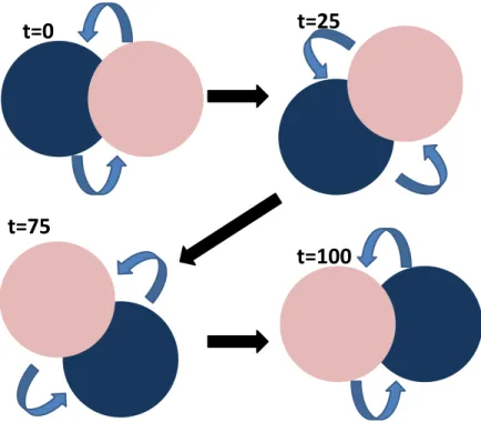
5.8.1 Rotating Circular Gaussian Drift . . . 168
5.8.3 NOAA Dataset . . . 172
5.9 Drift Detection using the Hellinger Distance . . . 174
6 Conclusions
184
6.1 Contributions of this Work . . . 1846.2 Summary of Findings . . . 186
6.2.1 Learning Concept Drift and Imbalanced Data . . . 186
6.2.2 Transductive Learning Ensembles . . . 188
6.2.3 Drift Detection using Raw Features . . . 189
6.3 Recommendations for Future Work . . . 189
6.3.1 Online learning of Under-represented classes in Data Streams . . . 189
6.3.2 Semi-Supervised/Transductive Learning in Nonstationary Environments190
References
192
Appendix
201
Appendix A: Learn++.NIEηvariation . . . 201List of Figures
2.1 Temperature variation over time . . . 15
2.2 Simple drift example . . . 16
2.3 Probability of sampling from different sources (gradual) . . . 20
2.4 Probability of sampling from different sources (reoccurring) . . . 20
2.5 SMV error as a function of classifiers . . . 21
3.1 Learn++pseudo code . . . 36
3.2 DWM pseudo code . . . 40
3.3 SEA pseudo code . . . 42
3.4 Cost-sensitive Boosting for Concept Drift . . . 46
3.5 Relationships in machine learning scenarios . . . 48
3.6 Shewhart drift detection algorithm . . . 49
3.7 Log-likelihood CUSUM test for drift detection . . . 51
3.8 SMOTE algorithm pseudo code . . . 55
3.9 SMOTE example . . . 56
3.10 SMOTE applied to checkerboard data . . . 57
3.11 Bagging ensemble variation algorithm pseudo code . . . 59
3.12 Bagging variation for imbalanced datasets . . . 60
3.13 SMOTEBoost pseudo code . . . 63
3.14 DataBoost-IM pseudo code . . . 65
3.16 SERA pseudo code . . . 70
3.17 MuSERA pseudo code . . . 73
3.18 Learn++.NSE pseudo code . . . 75
3.19 Time-adjusted weighting scheme . . . 77
4.1 Learn++.CDS pseudo code . . . 81
4.2 Learn++.NIE pseudo code . . . 84
4.3 Weight Estimation Algorithm (WEA) pseudo code . . . 92
4.4 Expectation Maximization for Gaussian Mixtures . . . 95
4.5 Hellinger Distance Between Two Gaussian Distributions . . . 98
4.6 Evolution of a binary classification task with two drifting Gaussian distributions . . . 99
4.7 Hellinger distance example of GaussCir . . . 100
4.8 Hellinger Distance Drift Detection Method . . . 102
5.1 Confusion matrix . . . 112
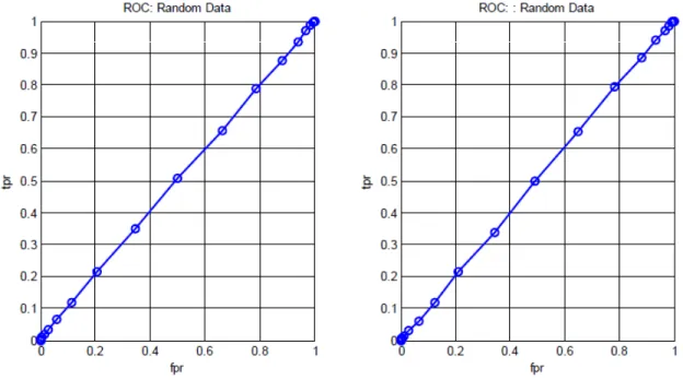
5.2 ROC curves for randomly labeled data . . . 116
5.3 ROC curves for covtype data . . . 117
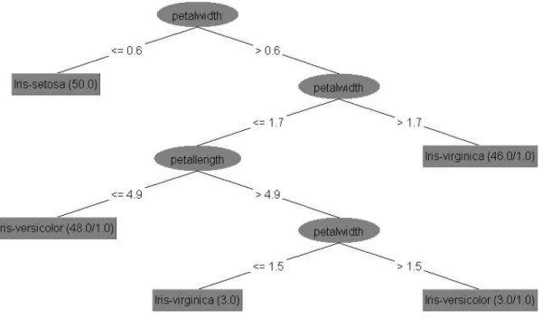
5.4 Visualization of a decision tree . . . 119
5.5 Rotating checkerboard dataset . . . 122
5.6 Recall for Learn++.CDS with varying imbalance . . . 124
5.7 Raw Classification Accuracy for Learn++.CDS with varying imbalance . . 125
5.8 Concept Drift Algorithms Evaluated on Checkerboad Data . . . 128
5.9 Learn++.NIE Algorithms Evaluated on Checkerboad Data . . . 129
5.10 Baseline Algorithms Evaluated on Checkerboard Data . . . 130
5.11 Learn++weight evolution on Guass . . . 131
5.13 Learn++.CDS evaluated on Spiral Data . . . 134
5.14 Learn++.NSE and SEA evaluated on Spiral Data . . . 136
5.15 Learn++.NIE family of algorithms evaluated on Spiral Data . . . 137
5.16 Baseline algorithms evaluated on Spiral Data . . . 138
5.17 Learn++weight evolution on Spiral Data . . . 139
5.18 Posterior probability of a Gaussian drift scenario . . . 141
5.19 Concept Drift Algorithms Evaluated on Gaussian Data . . . 143
5.20 Learn++.NIE Algorithms Evaluated on Gaussian Data . . . 144
5.21 Baseline Algorithms Evaluated on Gaussian Data . . . 145
5.22 Learn++weight evolution on Guass . . . 146
5.23 Shifting hyperplane experiment . . . 147
5.24 Concept Drift Algorithms Evaluated on a Shifting Hyperplane Dataset . . . 149
5.25 Learn++.NIE Algorithms Evaluated on a Shifting Hyperplane Dataset . . . 150
5.26 Baseline Algorithms Evaluated on a Shifting Hyperplane Dataset . . . 151
5.27 Learn++weight evolution on SEA . . . 152
5.28 Learn++.NSE weight distribution . . . 153
5.29 Concept Drift Algorithms Evaluated on the Elec2 Dataset . . . 155
5.30 Learn++.NIE Algorithms Evaluated on the Elec2 Dataset . . . 156
5.31 Baseline Algorithms Evaluated on the Elec2 Dataset . . . 157
5.32 Learn++weight evolution on Elec2 . . . 158
5.33 Distribution divergence of of the NOAA database . . . 159
5.34 Concept Drift Algorithms Evaluated on the NOAA Dataset . . . 160
5.35 Learn++.NIE Algorithms Evaluated on the NOAA Dataset . . . 161
5.36 Baseline Algorithms Evaluated on the NOAA Dataset . . . 162
5.38 WEA vs. Learn++.NSE on Rotating Circular Gaussian Drift . . . 170
5.39 WEA vs. Learn++.NSE on Rotating Circular Gaussian Drift with Failure . 171 5.40 WEA vs. Learn++.NSE on Rotating Triangular Gaussian Drift . . . 173
5.41 WEA vs. Learn++.NSE on Rotating Triangular Gaussian Drift with Large Bias . . . 174
5.42 WEA vs. Learn++.NSE on NOAA Dataset . . . 175
5.43 Evolution of the rotating checkerboard dataset . . . 177
5.44 Evolution of the circular Gaussian drift . . . 178
5.45 Evolution of the RandGauss drift . . . 179
5.46 Error evaluation of the on-line na¨ıve Bayes classifiers with HDDDM (Part 1) 180 5.47 Error evaluation of the on-line na¨ıve Bayes classifiers with HDDDM (Part 2) 181 5.48 Location of drift points as detected using the HDDDM . . . 182
A.1 Learn++.NIEηvariation on Gaussian data . . . 201
A.2 Learn++.NIEηvariation on SEA data . . . 202
A.3 Learn++.NIEηvariation on Elec2 data . . . 203
List of Tables
2.1 Incremental learning algorithm requirements . . . 12
3.1 Summary of FLORA family of algorithms . . . 39
3.2 Weight update equations for the different boosting schemes . . . 46
5.1 Algorithm Summary on Checkerboard Data . . . 127
5.2 Algorithm Summary on Spiral Data . . . 139
5.3 Mean and standard deviation Gaussian drift over time . . . 140
5.4 Algorithm Summary on Gaussian Data . . . 146
5.5 Algorithm Summary on Shifting Hyperplane Data . . . 154
5.6 Algorithm Summary on Electricity Pricing Data . . . 159
5.7 Algorithm Summary on NOAA Weather Data . . . 164
5.8 Summary of the OPM ranks of all the algorithms on all datasets . . . 165
5.9 Hypothesis testing for concept drift & class imbalance algorithms . . . 168
5.10 Mean and standard deviation Gaussian drift over time . . . 172
5.11 Datasets used for HDDDM experimentation . . . 176
Chapter 1
Introduction
Pattern recognition and machine learning is the process of taking in raw data and making a decision based on the category or class of the pattern [1]. Once we are provided a new (unlabelled) instance we wish to give a membership to the new data without the aid of a human. The ultimate goal in computational intelligence is to develop an algorithm that has the ability to mimic the brain-like intelligence, where in the context of machine learning is referred to as an adaptive and intelligent system (AIS).
The process of identifying patterns is crucial in the human thought process and has allowed for the evolution of our neural and cognitive systems. Our cognitive systems
allow for the learning of new knowledge when it is presented to us. Neural plasticity is
the learning and development of our neural systems in response to a new experience [2]. Plasticity allows for the acquisition of new information, so it seems intuitive that some form of plasticity be integrated into the learning machine if it is to react similar to human-like
intelligence. Neural stability is the retaining of information that has been previously
learned and is another valuable quality for a learning machine. Therefore, if we want the learning machine, or AIS, to have some brain-like intelligence properties, it is imperative to retain existing knowledge when relevant and learn new knowledge that becomes available over time.
In this thesis, the focus is on learning large amounts of data over time and the
environments from that may be dynamic in nature with unbalanced data. Dynamic
interchangeably throughout this thesis. Concept drift occurs when the statistical properties that govern the joint probability distribution change as a function of time. Unbalanced data, or imbalanced data, refers to an unequal representation of classes in a pattern recognition problem. There are typically two types on class in an imbalanced pattern recognition problem, majority (negative) and minority (positive). The majority (negative) class corresponds to a class or set of classes that is the large majority of the instances in a dataset. The minority (positive) class is under-represented in the training data. The minority class is typically of greater importance than the majority class to the pattern recognition problem.
Traditional machine learning theory presented in the classical texts generally assumes the classification algorithm is learning from a fixed yet unknown distribution [1, 3–5]. Assuming such a distribution may not be a valid assumption when the data come from
dynamic environments. While the classical texts provide a sound theory of machine
learning, they do not address the problems faced in many real world applications such as semi-supervised learning [6], imbalanced data [7], biased training/testing distributions [8] and incremental learning [9–11]. In this thesis, we focus on incremental learning, concept drift and class imbalance.
1.1
Problem Statement
The problems addressed in this thesis cover three main topics: incremental learning,
concept drift and class imbalance. Each one issue is studied individually as well as
combining them into a single composite problem. Each problem requires its own specific methods for evaluation. We use the following setting: data are presented sequentially in batches with a set of labels for training. After training is complete, a testing data set is then presented to the algorithm where the class labels are not available until after the algorithm
has been updated. Most importantly, we assume that the joint probability distribution of
the data and labels at timet,pt(x, ω), is not the same as the joint probability distribution at
timet+ 1,pt+1(x, ω).
1.1.1 Concept Drift
Concept drift occurs when the statistical properties that govern the distribution of the data change over time. This change could be caused by a hidden context, which may never be fully understood. Even though the reason why the distribution of the data are changing may not be fully known, an algorithm must take action in order to track and learn the drifting concepts. Traditional machine learning algorithms are not designed for learning in the presence of concept drift [1, 3, 4]. Thus, learning in nonstationary environments (i.e., in the presence of concept drift) requires that new methods be developed. Learning concept drift increases the difficulty of the classification task as the stability-plasticity dilemma needs to be more directly addressed. This work extends the effort set forth by Polikar, Muhlbaier, and Elwell [12, 13], which is review in Chapter 3. Concept drift is enjoying increased attention as the applications that generate nonstationary data become more prevelant in the real-world.
1.1.1.1 Examples of Concept Drift
Applications that generate drifting data are increasingly becoming more prominent in real-world learning scenarios. This section presents some applications where concept drift is found.
Consumer Ad Relevance: Consider an application that tracks which ads are most relevant
to a particular user’s interest. Customer interests are known to change – ordrift– over time,
express interest may no longer be relevant. Thus, the algorithm designed to determine the relevant ads must be able to monitor the customer’s browsing habits and determine when there is change in the customer’s interest.
Spam E-mail Detection: E-mail spam, commonly referred to as junk e-mail, are identical e-mails sent in bulk to a large list of recipients. This form of e-mail is unsolicited and the number of spam e-mails has been steadily increasing since the inception of e-mail. In the pattern recognition realm, our goal is to identify e-mails that resemble spam. Spam e-mails, however are not all identical and change over time. For example, a user may receive spam e-mails trying to get them to buy pharmaceutical drugs; however, as time goes on the focus drifts to weight loss drugs and casino ads. This change in features of spam (pharmaceutical
drugs→weight loss drugsL
casino ads) must be identified.
Other applications that call for an effective change or drift detection algorithm can be expanded. Changes in electricity demands, financial data analysis, and climate data analysis are all examples where change or drift detection is needed such that the learner may take an appropriate action.
1.1.2 Class Imbalance in Data
Class imbalance occurs when a (rare) class is severely under-represented in the training and testing datasets. Often, the rare (minority) class is more important to the pattern recognition task than the majority class. Learning from imbalanced datasets is very difficult for several reasons: (a) the primary class is under represented and may not provide information into the full feature space of the class, (b) traditional machine learning algorithms tend to bias themselves toward the majority class due to the optimization of an objective function, and (c) the misclassification of a minority class instance generally incurs more penalty than the majority class. Due to the issues associated with learning an imbalanced class problem,
we need to evaluate different measures to analyze the algorithms performance. Overall accuracy is generally used to measure the performance of an algorithm for concept drift. In fact, error is typically used to track and detect when drift is present in a stream of data. However, overall accuracy is no longer an accurate assessment of how well the algorithm is performing. For example, consider a dataset that contain 20 minority (positive) and 980 majority (negative) instances. If a classifier obtains 2% error on the dataset, it tells us very little about how well the classifier identified 20 minority instances. Error will be biased towards the majority class and error will not be adequate enough to access an algorithms
ability to recall the minority as well as majority class. Thus, we need to use statistical
measures other than accuracy/error when we evaluate algorithms on imbalanced data.
1.1.2.1 Examples of Class Imbalance
Datasets that contain imbalanced data are found in many real-world applications. This section presents some applications where imbalanced data is found.
Credit Card Fraud Detection: Consider a computer software program that is required to label whether or not a customer’s transaction is fraudulent or legitimate (as described in [16]). The fraudulent class in this application is severely under-represented. The majority class is likely be learned very well since the vast majority of transactions made every day by customers are legitimate. However, our primary task is to be able to identify the fraudulent transactions that are underrepresented in the training/testing data (imbalance is good for the customer / bad for the computer scientist).
Breast Cancer Classification from Mammograms: Consider the situation where a university is awarded a grant to improve the classification systems for breast cancer for younger patients as the detection is slightly more difficult in the early stages (say 30-39 years old). The primary objective of this project is to classify individuals as cancerous
(positive) or healthy (negative). The data for the project are provided by a hospital in the region and comes from the last 10,000 women between the ages of 30-39 who received a mammogram. According to the National Cancer Institute, only 0.43% of patients between 30-39 test positive for cancer (about 1 in 233) [17]. Thus, approximately 43 out of the initial 10,000 women can be used to build a model of the cancerous population. We typically find that classifiers bias themselves to the majority class (in this case the healthy patients) and
perform poorly on the positive (minority) class. Consider a classifier that obtains 20%
accuracy on the positive class and 100% accuracy on the negative class. This means 35 patients who have breast cancer will be labelled as healthy and 9957 healthy patients are
correctly identified, while the overall accuracy is(8 + 9957)/100000 = 0.9965. The high
performance is quite deceiving when the the accuracy on the minority class becomes the focus of the pattern recognition.
1.1.3 Incremental Learning of Data
The learning machine solution presented in this thesis are geared towards learning from streaming data over time, where concepts that define the problem may change over time. However, it is clearly infeasible from a computational point of view to retain all of the data due memory limitations. Moreover, we may no longer have access to the previous (old) data thus rendering any algorithm that needs access to it useless in such an application. Incremental learning requires an algorithm that is capable of learning from new data (that may introduce new concept classes), while retaining the previously acquired knowledge without requiring access to old datasets. One simple solution would be to train a new model every time data are presented and discard the old model, but this solution is rather na¨ıve in nature and incurs some detrimental results as discussed in the Background section of this thesis. Multiple classifier systems (MCS) or ensemble systems can be utilized to expand
our knowledge base (i.e., add to the ensemble) and retain old knowledge from previous
time (i.e., knowledge saved in the ensemble). This raises stability-plasticity dilemma
hinted earlier [18]. The classifiers within the ensemble are models for an environment at a different point in time thus leading to the use of old models based on their relevance in recent time. Ensemble systems have been shown to provide a good balance between stability and plasticity, which is one of the primary influences for using them in this work. The vast majority of the work done in incremental learning makes the assumption that the batches of data presented to an algorithm over time are coming from a static (i.e., fixed yet unknown) distribution. In other words the distribution is static.
1.2
Scope of Thesis
Combining concept drift and class imbalance into one learning problem has been
under-explored in machine learning literature. Traditionally, either concept driftor class
imbalance is addressed, rarely both. Furthermore, many concept drift algorithms perform poorly when imbalanced learning scenarios are present. Here we consider performing
poorly as an indication of how well the algorithm does onallthe classes.
It is important that research be carried out in this area for several reasons: many learning scenarios where concept drift is present may also contain class imbalance, and there are no truly incremental learning algorithms for this problem to the best of the author’s knowledge.
1.2.1 Concept Drift + Class Imbalance Applications
The classification of fraudulent credit card charges as presented in Section 1.1.2.1 may also be converted into a problem that contains both concept drift and class imbalance. Consider detection of fraudulent credit card charges as a function of time. In this example let’s assume we are provided labelled training data for updating our algorithm and field data
for classifying charges every year. The raw features in this example are derived from the amount of the transaction, distance from the customers’ residence, information on past purchases, time of the year and income of the customer.
Class imbalance is present in the training set simply because the fraudulent transactions occur far less often than a legitimate transaction. Now the features that describe the transactions may change over time and the change could be abrupt or gradual. For example, consider an individual who has a simple life-style and only buys essential goods. There may be a slight upward trend in the transaction amount because of inflation in the economy and varying prices in consumer products. Abrupt changes may occur when there is a crash in the stock market, change of occupation yield a change in the customers’ income, or changing patterns in the customer’s interests.
1.3
Summary of Contributions
This work presents an analysis of new algorithms that are capable of handling incremental
learning, concept drift and class imbalance at the same time. Two new algorithms,
Learn++.NIE and Learn++.CDS, have been developed specifically for this learning
scenario. Three variations of Learn++.NIE are presented as well. We then present a
transductive learning ensemble for concept drift. Finally, a drift detection algorithm is presented. The core portions of this thesis can be summarized as:
1. Analysis of a new set of incremental learning algorithms that learn from drifting
concepts and imbalanced classes, simultaneously. Two primary algorithms,
Learn++.NIE and Learn++.CDS, are presented along with three variations of
Learn++.NIE.
algorithm.
3. Empirical analysis of Learn++.CDS
4. A transductive learning algorithm for incremental learning in nonstationary environments. This ensemble algorithm attempts to estimate the weights of the Bayes optimal set of discriminant functions.
5. A drift detection algorithm for incremental learning scenarios using a difference in Hellinger divergence between two distributions.
Portions of the work presented in this thesis has appeared at the IEEE International
Conference on Pattern Recognition (ICPR2010), the IEEE World Congress on
Computational Intelligence (WCCI2010), and the IEEE Symposium on Computational Intelligence in Dynamic and Uncertain Environments (CIDUE2011).
1.4
Organization of this thesis
Chapter 2 provides a background into the problems encountered in incremental learning, concept drift and class imbalance. Chapter 3 follows with a comprehensive literature survey for algorithms that can handle incremental learning, concept drift, class imbalance and a fusion of the fields. Chapter 4 describes several new approaches to learning in such environments as well as a tranductive algorithm for concept drift and a drift detection method utilizing a divergence measure. Chapter 5 presents a set of synthetic and real-world experiments to evaluate the strengths and weaknesses of the algorithms presented in Chapter 4. Finally, a summary of conclusions and suggestions for future work are laid out in Chapter 6.
Chapter 2
Background
This chapter introduces the fundamental issues associated with incremental learning from concept drift and classes that are severely under-represented. Each issue is evaluated individually before forming a fusion of the problems, which is the core portion of this thesis. Running examples are presented and used throughout this thesis to convey key problems in machine learning.
2.1
Incremental Learning
Incremental learning is a useful and practical technique of learning new data over
time. Learning incrementally is not only useful because it allows us to refine our
models/classifiers over time, but one can make the claim that we rarely get access to the entire feature space in one dataset. Rather we are presented with portions of the overall feature space in each batch of new data. Thus, an incremental learning algorithm allows learning of the entire feature space although the entire space has not been observed in any one dataset. Because of incremental learning, we may update, or add to, our knowledge base as more data are provided. Multiple classifier systems (MCS) provide a rational solution [11, 19]. A more Neolithic approach to learning from new data is to simply
generate a new model and throw away the old knowledge. This is known ascatastrophic
forgettingand typically leads to undesirable results [20].
to the learning algorithm at evenly spaced intervals. At the end of every season, we must use this new information to update the mode. In the scenario described, not only is incremental learning vital, but also learning from concept drift as the feature describing the data drifts over of time. Concept drift in weather prediction is discussed in more detail in Section 2.2. The definition or criteria for an incremental learning algorithm may vary from author to author and for this reason we clearly specify our criteria for an incremental learning algorithm [11, 21]. As an example, some authors do not consider holding onto minority class data as a violation of the one pass requirement in definition of incremental learning. Minority class data refer to the class that are under-represented in an imbalanced dataset. The concept of imbalanced data is discussed in more detail in Section 2.3. The authors’ justification in [21] is that if the imbalance is large enough, then the physical memory usage required to store the data is extremely small and can therefore be accumulated over time. However, holding onto data, regardless of the class, for later use is in violation of the incremental learning definition in [11]. Therefore, we define an incremental learning algorithm as being able to learn additional information from new data when it becomes available, without requiring access to previous data, while preserving previously acquired knowledge [11]. Their criteria for incremental learning can be extend upon by including Kuncheva’s suggestions for an algorithm that learns from concept drift, to include limited processing time and any-time learning [22]. Table 2.1 summarizes the typical incremental learning requirements for learning in the presence of concept drift [11, 22, 23].
The definition of incremental learning requires that an algorithm is able to learn new
knowledge and retain old knowledge. This brings rise to the stability-plasticitydilemma,
which are generally two conflicting objectives [18]. Carpenter and Grossberg proposed a solution in Adaptive Resonance Theory (ART) [24]. ART was originally developed as an unsupervised neural network for incremental learning of binary input patterns. The
Table 2.1 : Incremental learning algorithm requirements
Requirement 1 One pass learning: The learning algorithm shall not require access to previous databases.
Requirement 2 Learn new knowledge: Build upon the current model when a new dataset is made available to the algorithm.
Requirement 3 Preserve previous knowledge: Knowledge shall not be discarded/forgotten from past learnt databases.
Requirement 4 Limited processing: Each batch should be processed in a small time regardless of number of the examples processed in the past.
fundamental theory of ART has been expanded to develop unsupervised neural networks for continuous inputs (ART-2), implementing fuzzy logic into ART’s pattern recognition (Fuzzy ART), implementing a supervised ART model for prediction (ARTMAP), and implementing fuzzy logic in ARTMAP (fuzzy ARTMAP) [10, 25–27].
The algorithms proposed and presented in this thesis are all incremental learning algorithms, where new training data are presented in batches over time. We refer to each
presentation of new data as time stamps. Incremental learning algorithms are different
than on-line learning algorithms as on-line learning requires that a classifier is updated with each new instance presented. Examples of on-line learners are na¨ıve Bayes [1, 5], Dynamic Weight Majority (DWM) [28], On-line Nonstationary Boosting (ONSBoost) [29], and Hoeffding decision trees [30, 31]. On-line learning algorithms typically maintain a good level of plasticity at the cost of stability while the opposite is true for an incremental learner.
2.2
Concept Drift
Traditional learning algorithms, such as Adaboost [32, 33] and Support Vector Machines (SVM) [34], assume the data defining the concepts are being sampled from a fixed yet
unknown distribution. If the test data distribution varies as a function of time (i.e., training set is sampled from a different distribution than the testing set), the theoretical error bound
of AdaBoost will not hold. Thus, we present a problem referred to as learning under
concept drift or innonstationary environments. Concept drift is the phenomenon of data
changing over time. This drift/change can be caused by a number of different factors governing the learning problem, however, models that address this change must be adaptive in order to remain relevant predictors. Concept drift is a difficult problem in machine learning where the learning scenario that the concepts (classes) of interest may depend on some hidden context [35, 36]. The drifting concepts in the data may be slow, fast, abrupt, gradual, cyclical or a combination [22, 37] and studies performed in information retrieval have indicated that target concepts may change at several different speeds over time [38]. The nature of why drift is present may be understood, yet the algorithm being applied for a problem with concept drift must track the drift to be an accurate predictor on new concepts or probability distributions. Learning in nonstationary environments has been receiving increasing attention over the past several years as more Master’s and Ph.D. theses focus on concept drift [13, 15, 23, 30, 39–42].
Any algorithm that does not make the necessary adjustments to changes in data distribution will fail to provide satisfactory generalization on future data, if such data does not come from the distribution on which the algorithm was originally trained. Recall the application that tracks a user’s web browsing habits to determine which ads are most relevant for that user’s interest. Tracking user interests have been studied in [14, 43–45]. Yandex.Direct is an advertising network that is designed specifically to take into account user interests when displaying ads [46]. Thus, an algorithm designed to determine the relevant ads must be able to monitor the customer’s browsing habits and determine when there is change in the customer’s interest. User interests may also be categorized as
short-term or long-term as described by ˇZliobait˙e [15]. ˇZliobait˙e gives an example where an individual working on a class project will change their browsing habits for a short period of time until the project is finished. Long term interests may include following a sport like football. Applications that call for an effective change or drift algorithm can be expanded: analysis of electricity demands, financial data analysis, and climate data analysis are all examples of nonstationary applications where change or drift detection is needed so that the learner can take an appropriate action.
Changes in a hidden context may not be the only cause of a changing concept, but may also cause a change in the underlying distribution of the data. Consider developing a pattern recognition algorithm that predicts whether or not it rained on any given day. A team of informed meteorologist interns determine there are several discriminating features to aid in predicting if it rained on the day the data was collected. The interns job for the summer is to gather data and pass it along to a team of researchers involved in machine learning. The data are used by those involved in machine learning group to generate a classifier whose sole purpose is to predict rainy days. The concept of a rainy day does not change. Either it rained or it didn’t rain on any given day when the data were collected. Now, new data are collected throughout the fall/winter months and classified with the rainy day model developed with the summer season data. It’s very likely, depending on the physical environment, that the features of the new data could be radically different than those used
for training due to changes in temperature, humidity, visibility, barometric pressure, etc∗.
The purpose of the classifier is still the same, predicting rainy days, yet new data from the fall/winter are presented to the classifier that could not have possibly been learned. Thus, the underlying distribution that governs the data has drifted as a function of time. This may cause the classifier’s error to be unacceptable with the new distribution that governs
0 1000 2000 3000 4000 5000 −20 0 20 40 60 80 100 time stamp temperature
(a) Drift over 5000 days
0 50 100 150 200 250 300 350 400 −10 0 10 20 30 40 50 60 70 80 90 time stamp temperature
(b) Drift over 365 days
Fig. 2.1 : Drift in average daily temperature. Data is acquired from the NOAA [47].
the data. Fig. 2.1 presents the average daily temperature in the National Oceanic and Atmospheric Administration (NOAA) weather database over 5,000 days and 365 days. In this example, the rainy day model must be adaptively updated to accurately predict on new data throughout the year.
The effects of concept drift can be analyzed through Bayes theorem in Eq. (2.1) & (2.3)
wherep(x)is the evidence of a random variablex,p(x|ωj)is the likelihood,P(ωj)is the
prior probability ofωjandP(ωj|x)is the posterior probability. This relationship is derived
from the joint probability distribution of xand ωj, namely: p(x, ωj) = p(x)P(ωj|x) =
p(x|ωj)P(ωj). The subscript,t, in Eq. (2.1, 2.2, 2.3) denotes a time stamp when the Bayes
posterior probability is computed. Simply, using any one of the terms in Bayes theorem is not enough to be certain that drift is present in the data.
Pt(ωj|x) = likelihood z }| { pt(x|ωj) prior z }| { Pt(ωj) pt(x) | {z } evidence (2.1)
Fig. 2.2 : Simple drift example pt(x) = c X i=1 pt(x|ωi)Pt(ωi) (2.2) Pt(ωj|x) = pt(x|ωj)Pt(ωj) Pc i=1pt(x|ωi)Pt(ωi) (2.3)
The evidence in Bayes theorem, Eq. (2.2), is the probability that the random variable
x(measurement) will even occur regardless of the class membership forx. The evidence
term may be written that as a summation over all classes of the product of the likelihood and prior probability as stated in Eq. (2.2). While it may be possible to use the evidence as a method to detect drift for a particular problem, it certainly is not enough for the more general drift detection scenario. For example, consider a uniform distribution of data over
two features,x = [x1, x2]T, and there is a linear separation between the two concepts as
shown in Figure 2.2(a). At a later point in time, the plane separating the two concepts shifts up to the location in Figure 2.2(b). The probability distribution of the data in this example
never changed when the plane shifted its location thus, p(x) never changed even though
Another possibility is that not just a single component of Bayes theorem is changing; there may be drift where two of the components in Bayes theorem are drifting with time [48]. This makes it very difficult to know what is changing unless there access to a massive amount of the data at each time stamp, which is simply infeasible to process and estimate the components of Bayes theorem, particularly for high dimensional data [1].
Bayes theorem may be used to describe three different concept drift scenarios. Concept drift may appear in one of three ways:
1. Class priors,P(ωi), change over time.
2. The likelihoods,p(X|ωi), may change.
3. The posterior probability,p(ωi|X), may change.
There are several terms for categories of concept drift, namely real and virtual drift.
Real drift is a change in the posterior probability distribution given by p(ωi|X). Virtual
drift is change in the distributions of one or several classes given byp(X|ωi). Dual change
occurs when both P(ωi) and p(X|ωi) change as a function of time. Regardless, of real,
virtual or dual change an algorithm must effectively process data to take an appropriate action when change is signaled or new data is processed.
2.2.1 Methods of Handling Concept Drift
A na¨ıve approach to learning from concept drift is to simply discard a classifier when new data are presented and generate a new classifier. Therefore, data are classified only with the newest classifier. This approach does not save any information about old environments,
which can be useful for a future classification task. Such an approach leads tocatastrophic
forgetting[20].
data, either one instance or one batch at a time. There are two types of approaches for
drift algorithms in such streaming data: inpassive drift algorithms, the learner assumes –
every time new data become available – that some drift may have occurred, and updates the classifier according to the new data distribution, regardless whether drift actually occurred.
In active drift algorithms, the algorithm continuously and explicitly monitors the data to
detect if and when drift occurs. If – and only if – the drift is detected, the algorithm takes an appropriate action, such as updating the classifier with the most recent data or simply creating a new classifier to learn the current data.
2.2.2 Definitions of Concept Drift
In this section, the definitions of drift types are presented. The types of drift are distinct from one another and are used during the design of the synthetic experiments. We use the
notion of a source S1 generating data from a fixed distribution and source S2 generating
data from a fixed distribution that is different than S1. Let S1 be the initial source for
generating data. This is the same notation used by ˇZliobait˙e [15].
Sudden Drift or Concept Change: Concept change occurs at a point in time when
source changes fromS1toS2. Fig. 2.2 is an example of abrupt concept change that contains
an abrupt change when the hyperplane separating the two classes suddenly changes its location. The SEA experiment, described in Section 5.5.4, is a prime example of sudden drift [49].
Incremental Drift: Incremental drift contains multiple sources however the difference between the sources is very small. Thus, the drift is only realized when observed globally. The rotating checkerboard problem presented in [50], and further described in Section 5.5.1, uses incremental drift since each time stamp is a different source.
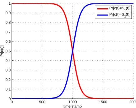
Gradual Drift: Gradual drift occurs when data are being drawn from two or more
similar sources within one time stamp. Generally, as time passes the probability of
sampling from S1 decreases as the probability of sampling from S2 increases. Consider
sampling from a data stream as presented in [23] whereS1 &S2 are two different sources
for two different data streams, t is the time, t0 is the point of change in the distribution,
c(t)is the stream generate by sampling streamsS1&S2, andWis the width of the change.
Then Eq. (2.4) can be applied as the probability of sampling from source S1 at time t
and Eq. (2.5) as the probability of sampling from sourceS2 at timet. The probability of
sampling from either source is shown in Fig. 2.3.
P (c(t) =S1(t)) = e−4(t−t0)/W 1 +e−4(t−t0)/W (2.4) P (c(t) =S2(t)) = 1 1 +e−4(t−t0)/W (2.5)
Reoccurring Concepts: Reoccurring concepts appear when several different sources are used to generate data over time (similar to incremental and gradual drift). However, unlike incremental and gradual drift, sources are used again to generate data at a future point in time. The checkerboard problem in [50] uses incremental drift with reoccurring concepts. A similar sampling scheme as described above may be applied to show a mixture of gradual drift with reoccurring concepts (see Fig. 2.4).
2.2.3 Ensembles for Concept Drift
Ensemble classifier based techniques have been widely studied since their inception [19, 51, 52]. The principle behind the ensemble decision is that the individual predictions combined appropriately, should have better overall accuracy, on average, than any
0 500 1000 1500 2000 0 0.1 0.2 0.3 0.4 0.5 0.6 0.7 0.8 0.9 1 time stamp Pr[c(t)] Pr[c(t)=S 1(t)] Pr[c(t)=S2(t)]
Fig. 2.3 : Probability of sampling from different sources under a gradual concept drift
scenario as computed using Eq. (2.4) and Eq. (2.5) wheret0 = 500andW = 250
0 500 1000 1500 2000 2500 3000 3500 4000 0 0.1 0.2 0.3 0.4 0.5 0.6 0.7 0.8 0.9 1 time stamp Pr[c(t)] Pr[c(t)=S 1(t)] Pr[c(t)=S 2(t)]
Fig. 2.4 : Probability of sampling from different sources under a gradual concept drift scenario with reoccurring environments
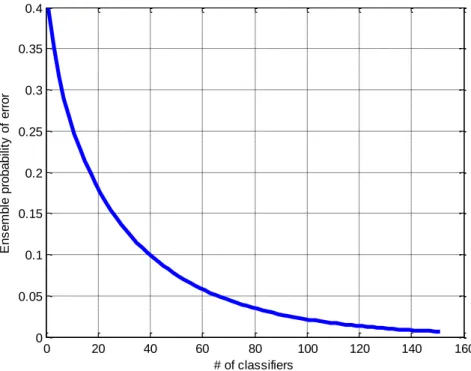
0 20 40 60 80 100 120 140 160 0 0.05 0.1 0.15 0.2 0.25 0.3 0.35 0.4 # of classifiers E n s e m b le p ro b a b ili ty o f e rr o r
Fig. 2.5 : Theoretical error vs. the number of classifier for an ensemble combined using
SMV. The error of each individual classifier isp= 0.4and is computed using Eq. (2.6).
individual ensemble member [53]. For the moment, consider the data are being drawn from a fixed yet unknown distribution. The concept of a varying distribution will be addressed after the following discussion on ensembles.
Consider a situation whereT classifiers are generated on a binary classification problem
where the classifiers have identical performance probabilities, and classifier outputs are independent of one another. Let the combination rule be a simple majority vote. If this is
true then Eq. (2.6) is the error probability of the majority vote wherepis the probability of
error. P(H(x)6=y) = T X k>(T /2) T k p k(1−p)T−k (2.6)
Eq. (2.6) shows that the classifiers only need to be slightly better than a random guess
for a binary classification problem (p <0.5). Ifp >0.5then the ensemble errorP →1as
T → ∞and ifp < 0.5then the ensemble errorP → 0asT → ∞. Therefore, classifiers
that areweakin performance may be used and combined to create a very strong decision.
The notion of using a set weak classifiers to form a strong hypothesis is the corner stone of Adaboost and boosting based approaches [33, 54]. Ensembles using boosting generate multiple classifiers on strategically chosen datasets, rather than random sampling as done in Bagging [55].
There are several reasons why an ensemble would be chosen over a single classifier solution, and the reasons have theoretical/practical motivations. First, which classifier to use in the absence of prior knowledge about a problem and is there a set of classifiers
that will perform better than others on a classification scenario? The No Free Lunch
theoremstates that if no prior information is available then no classifier is universally better
than any other classifier [56]. This includes random guessing. Second, ensembles may be extremely useful depending on the attributes or properties of the data. For example, ensembles may be used to simplify a problem by breaking a difficult problem into simpler problems. Consider generating a classifier on an extremely high dimensional dataset. A single classifier’s complexity may scale with the dimensionality of the data thus making the generation of a reliable single classifier on the data infeasible. Instead of a single classifier, generate multiple classifiers on different subsets of features thus reducing the complexity of the classifier trained on the subset. Third, single classifiers may not work well with data that are too little or too large in size. To work around this problem, ensembles can generate classifiers on multiple bootstrap datasets. A small dataset benefits from bootstrapping datasets because each classifier is generated on a different dataset sampled from the same distribution. If the cardinality of the data are too large then the entire dataset
can be divided into smaller datasets and a classifier is generated in the smaller dataset. All classifiers must be combined to form the ensemble hypothesis. Fourth, generating a single strong classifier may be infeasible due to computational costs. Generating a classifier that performs slightly better than random guess is easier. Ensemble-based approaches have been widely used in earlier efforts of our group (SPPRL): including posterior estimation [57], early diagnosis of Alzheimer’s disease [58], missing features [59], data fusion [60], and learning in nonstationary environments [12].
The aforementioned reasons provide justification for using ensembles when the data are drawn from a fixed yet unknown distribution. With certain modifications, the ensemble system can also be used in concept drift problems. In each ensemble based approach, a method for classifier combination in needed along with method to generate classifiers in
the ensemble. First, call theBaseClassifierto generate a new classifier when training data
are presented. Instead of generating a weak classifier, as done in Adaboost, concept drift algorithms should have a fairly strong classifier that serves as a model of the distribution of
data on which it was trained. Algorithms such as Learn++.NSE use this approach because
unlike Adaboost, Learn++.NSE is designed to learn from sequential batch data and the
classifier generated on each batch must have the ability to form a strong hypothesis on the data it was trained with.
Next, a combination rule should be selected to combine the outputs of the classifiers. Kuncheva presents an excellent analysis of ensembles and combination rules in her text,
Combining Pattern Classifiers[52]. The choice of combination rule depends on the types
of labels a classifier may return. Typically, classifiers outputs can be reduced down two
types: ahardorsoftlabel classifier. A classifier that returns a hard label provides support
only to the class it has selected for a given instance. The CART and C4.5 decision trees are examples of classifiers that provide hard labels. A classifier that returns a soft label
provides some support for each class the classifier was trained on. This level of support is generally an estimate of a posterior probability. The multi-layer perceptron neural network (MLPNN) and logistic regression are examples of classifier that provide a soft label.
Classifiers that return only hard labels limit the types of combination rules that can be used. For example, na¨ıve Bayes, sum, median and majority rules are quite popular combination rules. However, the na¨ıve Bayes rule cannot be used with classifiers that return hard labels as it needs a level of support for each class. The na¨ıve Bayes combination rule
is given by Eq. (2.7) where µj(x) is the ensemble support given to class j for instance
x, P(ωj) is the prior probability ofωj, and p(dk(x)|ωj)is the likelihood of the classifier
decisiondk(x)given classωj.
µj(x)∝P(ωj)
T
Y
k=1
p(dk(x)|ωj) (2.7)
In concept drift applications, a new classifier is typically generated at each time stamp. So, which voting scheme or combination rule is appropriate for concept drift problems? Since the distribution of data evolve over time, some classifiers will have lower error than others on the most recent environment. Therefore, one cannot assume that equal weights (i.e., sum or mean rule) would be the best selection if some are known to perform better than others on recent environments. Gao makes the claim that one cannot always assume that the distributions of most recent training data and the incoming testing data are alike, which is a true statement [61, 62]. However, if the data are evolving in a systematic pattern
(not stochastic) then simply assuming there is no information abouthow a classifier will
perform on a future distributionmay not be entirely true. Gao reaches this conclusion by
T X k=1 w2k (2.8) 1− T X k=1 wk = 0 (2.9) 0≤wk ≤1 (2.10)
The problem described is a constrained convex optimization that can be easily carried
out by forming a Lagrangian function,L(w, α, β, λ). By computing ∂w∂L
k is can be shown
thatwk = 1/T (i.e. uniform weighting).
However, using uniform weighting does not make practical sense with an ever-growing ensemble [13]. Gao’s algorithm will be used as a comparison to the proposed weighted voting scheme described later in this thesis.
This thesis focuses on weighted majority voting approaches. This combination rule
assigns a weight to classifier to use for voting. The weight is typically proportional to the classifier’s performance. Thus, if a classifier is performing well on recent environments, the weight will be large and if the classifier is performing poorly, the weight will be small. Since the concepts are evolving systematically, the classifier’s error in recent time can
serve as the basis for determining a classifier’s weight, as implemented in Learn++.NSE
[12]. However, when dealing with imbalanced data, error is no longer a reliable measure. This is discussed later in Section 4.2 where new measures are presented for determining a classifier’s voting weight.
2.2.4 Drift Detection
Concept drift algorithms generally fall into one of two categories: active or passive algorithms. In passive algorithms, the learner assumes that some drift has occurred since the last training session whereas active drift algorithms will seek to explicitly determine when the drift is present in the data. If drift is detected, the algorithm takes an appropriate action, such as updating the classifier with the most recent data or simply creating a new classifier to learn the current data. Drift detection algorithms typically fall into the active category of algorithm.
There are several schools of thought for designing a drift detection algorithm. First, one has to select a method or a set of drift descriptors to seek the presence of concept drift in data. Classifier error is one of the most popular indicators of drift in data [63,64]. Classifier error is commonly used under two primary assumptions:
• A classifier trained onD(t)will have a relatively constant error onD(t+1) andD(t+tq)
wheret+tq is any arbitrary time stamp in the future.
• The error of a MCS will have increasing accuracy as classifiers are trained on new
data.
where D(t) is the dataset at time stampt. Error may not be the only indicator of drift in
data. Some algorithms use raw features to determine when drift is present. Using the raw features to determine drift requires that a parametric or non-parametric method to model the distribution of the data. A parametric model makes assumptions about the distribution from which the data are drawn. Gaussian distributions are common assumptions to simplify calculations and as properties of the Gaussian distributions are well known. However, what if the data are not actually drawn from a Gaussian, but a mixture of Gaussians or a different distribution all together? Non-parametric models, such as kernel density estimators, do not
make any assumption about the distribution of the data.
Regardless of the selection of drift descriptors, an action is needed if drift is detected. After change is signaled, the algorithm (or a different algorithm run in conjunction with the drift detection method) should take an appropriate action. Actions can include discarding a classifier, generating a new classifier, updating classifier weights, or doing nothing.
2.3
Class Imbalance in Machine Learning
Class imbalance, sometimes referred to as unbalanced data, occurs when a dataset does not have an (approximately) equal number of instances from each class, which may be quite severe in some applications [65]. Unbalanced data research focuses on situations where the class balance is nowhere near 50%. Rather, severe class imbalance (1%, 2%, 5%, 10%, etc). The datasets with severe class imbalance requires that algorithms figure of merit is addressed in a different manor than if there were only concept drift in data. Consider datasets with imbalances of 1%, 2%, and 5% and a classifier is generated yielding performances of 99%, 98%, and 95%, respectively. The classifier used in this simple example can be a majority class classifier, which simply classifies a new instance with the label of the class that occurs most often. The majority classifier will have a high overall accuracy, which is generally a good quality, however it will not be able to identify any of the instances that belong to the minority class. From this very generic example, its clear that error is not a best statistic to identify how well the algorithm is performing across all classes. Therefore, researchers dealing with imbalanced datasets will typically present results with statistics other than overall error to access an algorithm on an experiment. Before analyzing measures other than error, let’s focus on issues associated with learning from imbalanced data.
2.3.1 Why Do Classifiers Perform Poorly on a Minority Class?
Class imbalance arises from the under representation of at least one class in a learning problem. The minority class is unfortunately the target class for many classification tasks. Recall the example of credit card fraud in Chapter 1. The number of legitimate transactions essentially dwarfs the number of fraudulent transactions. Then how can the fraudulent transactions be learned when there are so few instances and how the classifier resist biasing towards to majority class? The fraudulent class in this scenario is difficult to learn for couple reasons:
• there are so few instances that there may not be a clear representation of the minority
class feature space
• many classification algorithms tend to minimize an error function, which may not
favor learning a minority class.
The first point is obvious and is partially a motivation for incremental learning, however the second point is worth further discussion. Classifiers typically minimize a global error function during the training process and do not take information about the distribution of the data into account. As a result, instances from the majority class are classified with high accuracy whereas examples from the minority class tend to be misclassified. For example, algorithms such as the multi-layer perceptron neural network (MLPNN) minimize an error function, generally mean-squared error (MSE), during the training phase of the neural network [66]. So, if a classifier is likely to bias its decisions towards a majority class, what can be reduce this effect? Sampling methods, cost-sensitive learning models, and ensemble have demonstrated favourable qualities to avoid bias towards the majority class as discussed in Section 2.3.2, 2.3.3, and 2.3.4.
2.3.2 Sampling Methods
There are several popular methods of handling class imbalance. Some of the more popular
approaches to learn class imbalance occur at a data or algorithmic level [67]. The data
level approaches generally employ some form of sampling to generate a new dataset that is similar to using bootstrap datasets with ensembles. Simple data level approaches use random over-sampling of a minority class or under-sampling of the majority class to reduce the imbalance. The random sampling must be done with care for several reasons. A simple random over/under-sampling of a dataset to create a less imbalanced dataset comes with repercussions. A simple random under-sampling of a dataset will discard instances from the majority class. However, by throwing out instances from the majority class, risks discarding information that can be useful to the classification problem. Over-sampling on the other hand does not discard majority class data, rather it adds exact replicates of the minority class. Using this approach to re-balance a dataset runs the risk of generating a classifier that will overfit the minority class.
Synthetic sampling can be used to reduce the undesirable qualities in random
over/under-sampling of minority/majority class data. Synthetic sampling methods
generally oversample a data set; however the instances added into the new dataset
are synthetic, and not exact replicates of the minority data as performed in random
over-sampling. The synthetic data are generated such that they are ”similar” to other instances in the minority class population. Some synthetic sampling methods not only focus on the generation of synthetic data but also the location of the synthetic instances. For example, synthetic sampling methods may generate synthetic instances that lie near a decision boundary. The synthetic sampling methods have been shown to be less prone to over-fitting classifiers to the minority class.
Over/under or synthetic sampling does not guarantee that the minority class can be adequately learned. Rather, sampling is a fast, cost-effective method of generally increasing the performance on a minority class. Studies have shown that some classifiers on particular datasets are not affected by sampling methods. Regardless, many imbalanced datasets benefit from sampling. Popular sampling approach can be found in Section 3.3.1.
2.3.3 Cost Sensitive Learning
The sampling methods described in the previous section attempt to develop a new dataset that contains less class imbalance. Note, that sampling methods may not convert the imbalanced learning problem into one that is balanced, rather they create a less imbalanced learning problem. Cost-sensitive learning algorithms assign penalties based on a cost matrix, which represents the penalties for different possible correct/incorrect classifications. The cost matrix can be considered as a numerical representation of the penalty of classifying examples from one class to another. The objective of cost-sensitive learning is to generate a classifier that minimizes the overall cost, not error, on the training data set, which is usually the Bayes conditional risk [1, 7]. The cost-sensitive learning problems generally lend themselves better to theoretical analysis than sampling methods.
2.3.4 Ensemble Methods
Ensemble methods are not only popular for reducing error of the final hypothesis, but are also employed to learn an under-represented class. The last two sections have focused on using sampling or cost-sensitive learning to increase the performance on a minority class. Ensembles are widely used for learning class imbalance by combining multiple classifiers, sampling, and cost-sensitive learning. Several existing ensemble techniques minimize the overall cost during training, not the error. Several different ensemble methods
are discussed in more depth as the literature review of the class imbalance is presented in the next chapter.
2.4
Learning Concepts Drift from Imbalanced Data
Both class imbalance and learning with concept drift have been independently studied by the machine learning community. In fact, there are a number of workshops held every year
that focus specifically in this area of computational intelligence. Recently, the WCCI†,
CIDUE‡, ECML§, and PKDD¶have had sessions and/or tutorials dedicated to the problem
of concept drift. The SIGKDD journal had a dedicated issue specifically for learning problems with class imbalance. The increasing interest in these fields can be attributed to their vast areas of application, because most modern day machine learning problems experience some underlying change with time and classes are rarely distributed equally. We begin this section by presenting application areas that experience class imbalance and concept drift simultaneously.
2.4.1 Real-World Scenarios
Recall, the example of climate prediction analysis where the features are going to drift as a function of time, hence the reason. This application also faces class imbalance in many of these learning scenarios. Let’s consider an algorithm that is designed to predict whether or not it rained more than 3 inches on any given day. The algorithm must be able to track the drifting concept, but also must learn from a small amount of instance. How many days will experience rain fall greater than 3 inches? The specific number of days is not as important
†http://www.wcci2010.org/
‡http://www.ieee-ssci.org/2011/cidue-2011 §http://wwwis.win.tue.nl/hacdais2010/
as the ratio between the number of days it rained more that 3 inches and the number of days it did not. It is very likely that the number of days it did not rain 3 inches is much larger than the number of days it did not.
2.4.2 Learning in Harsh Environments
Typically, machine learning algorithms are simply not equipped to handle class imbalance or concept drift and the algorithms that are designed to handle harsh environments only focus on concept drift or class imbalance, not both simultaneously. Concept drift algorithms typically use error as a weighting measure or as an indicator of drift, but error is a biased measurement (biased towards a majority class). It is unreasonable to expect an algorithm designed for concept drift to be the ideal algorithm when dealing with class imbalance. In fact, the concept drift algorithm should be expected to have a very high overall accuracy while achieving a poor recall of a minority class. The poor performance on
a minority class is simply unacceptable since the minority class is usually thetarget class.
From the point of view for ensembles, error is generally the statistic used to determine a classifier’s voting weight, hence the reason for an ensemble biasing its decision towards majority classes. Part of the motivation for this thesis is to answer the question, can statistics other than error be used to produce a classifier voting weight and still able to achieve the following: 1) tracking drift concepts in nonstationary environments, and 2) increase the accuracy on a minority class.
The evaluation of algorithms on data with concept drift and class imbalance must be done in a way to demonstrate that the proposed approach can track drift concepts and learn a minority class. Maximizing the performance of an algorithms is not the primary objective of this work. The objective of this work is to effectively learn in the presence on concept drift while maintaining a strong performance on a minority class.
2.5
Summary
In this chapter we have described incremental learning, concept drift and class imbalance in detail. Examples have been presented for real-world learning scenarios that motivate each area of research. We have also presented reasonable logic about why classifiers designed for concept drift may perform poorly in imbalanced learning scenarios. Against this background, the next section introduces the prior work that has been performed in the computational intelligence community for incremental learning, class imbalance, concept drift, and a fusion of concept drift & class imbalance.
![Fig. 2.1 : Drift in average daily temperature. Data is acquired from the NOAA [47].](https://thumb-us.123doks.com/thumbv2/123dok_us/9788699.2470628/31.918.186.786.138.392/fig-drift-average-daily-temperature-data-acquired-noaa.webp)
![Fig. 3.5 : Relationship between knowledge transfer, time-series analysis, model adaptation and concept drift [15]](https://thumb-us.123doks.com/thumbv2/123dok_us/9788699.2470628/64.918.190.781.118.430/relationship-knowledge-transfer-series-analysis-model-adaptation-concept.webp)
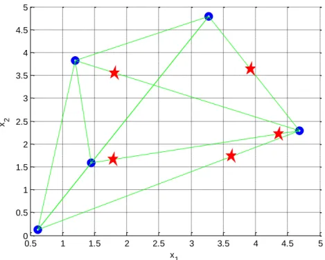
![Fig. 3.12 : Disjoint set formulation used the bagging ensemble variation [101]. The majority class (red circles) are divided in disjoint sets and combined with the minority class (blue triangle) to form a new dataset used to generate a classifier.](https://thumb-us.123doks.com/thumbv2/123dok_us/9788699.2470628/76.918.242.740.138.508/disjoint-formulation-ensemble-variation-majority-disjoint-combined-classifier.webp)