Article
Automatic 3-D Building Model Reconstruction from
Very High Resolution Stereo Satellite Imagery
Tahmineh Partovi1,* , Friedrich Fraundorfer1,2 , Reza Bahmanyar1 , Hai Huang3 and Peter Reinartz1
1 Remote Sensing Technology Institute (IMF), German Aerospace Center (DLR), 82234 Wessling, Germany 2 Institute for Computer Graphics and Vision, Graz University of Technology, 8010 Graz, Austria
3 Institute for Applied Computer Science, Bundeswehr University, 85577 Neubiberg, Germany
* Correspondence: [email protected]; Tel.: +49-152-55767747 Received: 27 May 2019; Accepted: 9 July 2019; Published: 11 July 2019
Abstract:Recent advances in the availability of very high-resolution (VHR) satellite data together with efficient data acquisition and large area coverage have led to an upward trend in their applications for automatic 3-D building model reconstruction which require large-scale and frequent updates, such as disaster monitoring and urban management. Digital Surface Models (DSMs) generated from stereo satellite imagery suffer from mismatches, missing values, or blunders, resulting in rough building shape representations. To handle 3-D building model reconstruction using such low-quality DSMs, we propose a novel automatic multistage hybrid method using DSMs together with orthorectified panchromatic (PAN) and pansharpened data (PS) of multispectral (MS) satellite imagery. The algorithm consists of multiple steps including building boundary extraction and decomposition, image-based roof type classification, and initial roof parameter computation which are prior knowledge for the 3-D model fitting step. To fit 3-D models to the normalized DSM (nDSM) and to select the best one, a parameter optimization method based on exhaustive search is used sequentially in 2-D and 3-D. Finally, the neighboring building models in a building block are intersected to reconstruct the 3-D model of connecting roofs. All corresponding experiments are conducted on a dataset including four different areas of Munich city containing 208 buildings with different degrees of complexity. The results are evaluated both qualitatively and quantitatively. According to the results, the proposed approach can reliably reconstruct 3-D building models, even the complex ones with several inner yards and multiple orientations. Furthermore, the proposed approach provides a high level of automation by limiting the number of primitive roof types and by performing automatic parameter initialization.
Keywords:automatic methods; 3-D building model reconstruction; digital surface model; exhaustive search; hybrid methods; satellite imagery
1. Introduction
Accurate three-dimensional (3-D) building models are highly demanded in many applications including urban planning, mobile communication network planning, mobile navigation systems, virtual tourism, cartography, disaster monitoring, and change detection.
These applications usually require frequent updating of 3-D building models in large scale which has increased the need for developing automated methods based on remote sensing data over the past decades. Dense 3-D point clouds or DSM provided by either airborne laser scanning techniques (light detection and ranging—LiDAR) or satellite/aerial stereo image matching is privileged since it allows easy discrimination of the elevated objects such as building from their ground-level neighbors. Although LiDAR and aerial imagery provide dense and accurate 3-D surface information, Remote Sens.2019,14, 1660; doi:10.3390/rs14111660 www.mdpi.com/journal/remotesensing
their availability is limited to a few specific locations in the world due to restrictions in data acquisition and authorization. By contrast, satellite images provide coverage of the whole globe with a high acquisition frequency. Furthermore, the rich semantic information contents of satellite images can enhance building detection and classification results. Despite all their advantages, to the best of our knowledge, satellite images have been used only by a few previous works for 3-D building reconstruction [1–4].
Relying on satellite imagery for 3-D building model reconstruction faces a few challenges due to scene and building boundary complexities, drawbacks of stereo satellite imagery, and stereo image matching errors. The low pixel resolution of satellite images relative to aerial images (approx. 0.5–1 m in PAN and 2–4 m in MS images), their low signal to noise ratio (SNR), occlusion problems due to their wide base lines, and image matching errors can particularly influence the accuracy of satellite-based DSM data. This can cause noise, artifacts, and imperfections (e.g., gaps) particularly at building edges [3,5] and can consequently affect the accuracy of automatic building reconstruction approaches. Dealing with the gaps and imperfections of DSM data, a number of previous works [6–9] applied interpolation methods; however, the results are still unsatisfactory due to the interpolation deficiencies such as blurring the building boundaries, which can impose imperfections to the building masks derived from the DSM data. In order to improve building masks, a number of previous research works proposed approaches based on various combinations of DSM data and very high-resolution (VHR) satellite images [1,3,10,11]. Grigilloi et al. [11] refined the nDSM-based building mask using nonlinear diffusion filtering, unsupervised classification, color segmentation, and region growing. Partovi et al. [12] refined the boundaries of building mask by applying a classification method (e.g., support vector machine—SVM [13]) to the primitive geometrical features (e.g., scale invariant feature transform descriptors—SIFT [14]) of their corresponding high-resolution PAN images. Later, Gharibbafghi et al. [15] proposed a fast and robust building mask refinement method based on multi-scale superpixel segmentation applied to DSM data and thereof VHR images. Noise in DSM of stereo satellite imagery can harden, extracting meaningful patterns from neighboring pixels resulting in inaccurate building geometric parameters (e.g., slopes and normal vectors). Dealing with this issue, some methods refined DSMs based on filtering techniques [16,17]. A method is proposed by [1,3] to extract accurate roof components (e.g., ridge lines and step edges) from VHR optical satellite images. Bittner et al. [18] proposed improving the DSM of satellite imagery by a conditional generative adversarial networks (cGAN) together with more accurate DSM data such as LiDAR-DSM and LoD2 (Level of details (LOD)1 and 2: LOD1 provides prismatic models generated from the extrusion of building outlines in their 3rd dimensions and LOD2 includes roof shape and structure.) -DSM. Duan and Lafarge [4] improved the DSM of satellite imagery by using 3-D reconstruction of the mesh-based models of the high-rise buildings with a flat roof type (LoD1).
In this paper, a novel automatic multi-stage hybrid method is proposed to reconstruct 3-D building models with LoD2 in the vector format using DSM and VHR optical satellite imagery. This approach handles noisy satellite-based DSM with no need for any direct improving the data. In addition, it extends the methods in References [12,19,20] to deal with building complexities and other dataset-related challenges. In order to evaluate the approach, it is used for reconstructing 3-D building models of four areas in Munich city (three areas are similar to that of Reference [12]). The results are evaluated qualitatively and quantitatively which shows that the proposed approach allows for reconstructing the buildings higher than 3 m and larger than 75 m2(300 pixels in the images with 0.5 m resolution).
This paper is organized as follows: Section 2gives a brief literature review on three main steps of building modeling—building detection, building outline extraction, and 3-D building model reconstruction—and points out the drawback of state-of-the-art methods regarding this topic. Section3
describes our proposed method for 3-D building model reconstruction in detail. In Section 4, experiments on four different areas with different urban complexity are carried out to validate feasibility and robustness of the proposed method. The results are evaluated qualitatively and
quantitatively. In this section, we discuss potentials and limitations of the method. Finally, Section5
concludes the paper. 2. Related Work
Many approaches have been proposed by recent research works to increase the automation level and to decrease the amount of human interventions [2,21,22]. The existing automatic 3-D building model reconstruction approaches can be generally categorized into model-driven, data-driven, and hybrid approaches. Model-driven approaches select the best fitting model to the 3-D point clouds or DSM data from a building library to represent the 3-D model of buildings [2]. The differences between the 3-D building model and 3-D point clouds are calculated based on a cost function such as normal or vertical distance. Nevertheless, data-driven approaches extract geometrical components (e.g., lines, corners, planes) from 3-D point clouds or DSM data provided and, subsequently, consider some geometrical topology between these components to form 3-D building models [22]. Hybrid approaches integrate the two former approaches. In hybrid approaches, a data-driven approach generally extracts the building roof features, such as ridge/eave lines, and other prior knowledge for a subsequent model-driven approach [23].
The preliminary steps in reconstructing 3-D building models from remote sensing data are detecting and discriminating building areas from other existing objects in the image scenes, such as vegetation and roads [10,21,24–28]. After detecting buildings, their 2-D outlines are extracted to be used in 3-D building model reconstruction. In order to extract building boundaries by fusing DSMs and high spatial resolution images, firstly, pixels on the boundaries of building mask can be traced based on the different methods such as the alpha-shape [29] and convex hull [30]. Next, the linear points are grouped into line segments and are simplified based on line fitting approaches such as Hough transform [31], random sampling consensus (RANSAC) [32], and sequential least square line fitting [12,33]. Some other methods use the rectangle fitting-based approaches such as minimum bounding rectangle (MBR) [34–37], reversible-jump Markov chain Monte Carlo (RJMCMC) [38], and a novel active shape detection approach [3]. Douglas Peucker algorithm [39] is a well-known method for simplification of polygon.
After detecting buildings and extracting their boundaries, their 3-D models are created using model-driven, data-driven, or hybrid-based building model reconstruction approaches. The important steps of the model-driven methods consist of building polygon decomposition, parametric roof library definition, and roof model selection. Model-driven approaches normally decompose the complex building polygons into simple rectangular structures, the so-called building primitives. Kada and McKinley [40] proposed a method to decompose building footprints into small sets of nonintersecting quadrilateral-shaped polygons, the so-called cells. Adequate subset of lines which are long enough in an assumed buffer are found and then extended infinitely for their proposed methodology. Later, Henn et al. and Zheng et al. [41,42] used a similar footprint decomposition method. This decomposition method results in many small cells which are not informative for 3-D building modeling from poor quality stereo satellite-based DSM. Vallet et al. [43] introduced a decomposition and merging method based on minimizing an energy function in the roof area with height discontinuities using DSMs of aerial imagery. Lafarge et al. [44] decomposed the rectangles extracted [45] during the regularization process by transforming neighboring rectangles into sets of connected quadrilateral or triangles. They then found the best configuration of the neighboring rectangles by the simulated annealing technique. The final quadrilaterals are partitioned further by detecting the height discontinuities from their inner DSM. This method is very efficient for dealing with low-quality datasets such DSMs of satellite imagery. However, it is complicated where a complex cost function needs to be defined. Arefi and Reinartz [1] decomposed footprints into rectangles based on ridge lines detected from satellite nDSMs and orthorectified PAN images. Extracting ridge lines where images have low contrast or incomplete DSMs will fail. Another similar method is proposed by Zheng et al. [23] in which building footprints were decomposed into sub-footprints by detecting the step edges from canny points on
the nDSM of LiDAR data. The sub-footprints are further decomposed by the ridge lines identified using watershed analysis and stream order algorithms from the nDSM of LiDAR data and VHR aerial images.
Parametric models describe roof primitives in libraries which are very important components in the model-driven methods. The defined libraries in the previous works are variable depending on the resolution of the data and common roof types in the study areas. Generally, the library consists of two parts of single-plane (e.g., flat and shed roofs) and multiplane roofs (e.g., gable, cross-gable, intersecting, half-hip, hip, pyramid, mansard, gambrel, dutch, and salt-box) [2,41].
Roof model selection is the process of fitting models into point clouds and selecting the most appropriate model from a library which minimize a cost function. Mass and Vosselman [46] proposed a new method for gable roof reconstruction by computing their parameters using the analysis of invariant moments of the 3-D point clouds of LiDAR data. The information on the roof type and shape parameters is computed by using the heights of the point clouds as weight functions in moment equations. Haala et al. [47] estimated roof plane parameters by segmenting the DSM of aerial images and by analyzing the surface normals and ground plane orientations of the segments. A similar approach was presented in Kada and McKinley [40] using LiDAR points of each cell. They determined the roof types according to the number of segments. Zheng et al. [23] also used a similar approach for roof type identification, in which the root mean square error (RMSE) between the DSM and corresponding points from the candidate roof model determines the quality of reconstruction. Poullis and You [48] computed the roof model parameters using a nonlinear bound-constraint minimization. During this optimization, a Gaussian mixture model (GMM) was used to detect and exclude outliers from the fitting plane, where the parameters of GMM were estimated using an expectation-maximization (EM) algorithm. Lafarge et al. [2] proposed a stochastic method for reconstructing 3-D building models from the DSM of satellite imagery (PLEIADES satellite data simulations with resolutions of 0.7 m). They used a Bayesian algorithm based on RJMCMC to decide the building model which best fitted the DSM data. Huang et al. [49] utilized generative statistical models to reconstruct 3-D building models from LiDAR data. The method finds the optimal combination of parameters by a stochastic search. Henn et al. [41] proposed a strategy for 3-D building reconstruction from a small number of LiDAR data points. This method estimates roof parameters by fitting the roof models and by estimating their parameters by M-estimator sample consensus (MSAC). It determines the most probable roof model by a support vector machines (SVM). Zheng and Weng [42] proposed a method based on LiDAR data and building footprints. They computed some morphological and physical parameters from a decomposed footprint. They then applied a decision tree-based classifier to these statistical features to classify the building footprints into seven roof types. According to the roof type, they calculated the roof model parameters based on the statistical moments of the points within the cells.
Another categorization of 3-D building reconstruction is data-driven approaches in which roof segments, boundaries, intersection lines, step edges, roof topology graphs, and regularization are necessary components for constructing polyhedron models. Most of the efforts in data-driven roof model reconstruction have been focused on the roof plane segmentation [21,50,51]. The point cloud segmentation methods, such as surface growing [29], triangulation irregular network (TIN) growing [46,52], and surface fitting techniques [53], turn roof surface points into planar, cylindrical, and spherical structures [54]. After detecting the roof segment regions, the adjacency between them is determined based on the closeness of two segments features such as edges [50], points [55], and intersection lines [22].
Ridge lines and step edges (height discontinuities) can be extracted regarding planar segments, adjacency, and topological relations. The step edge between two segments can be determined by analyzing the height differences on an orthogonal profile to the boundary of the segments [56]. Elberink [57] detected step edges by analyzing 2-D and 3-D relations between the adjacent segments which have no intersection line. Sohn et al. [58] developed a step line extractor, the so-called compass
line filter (CLF), which tracks all boundary points with height discontinuities on the adjacent clusters on the TIN. This process continues with thinning and computing the directions of the step edge lines. Rottensteiner and Briese [59] computed the intersection lines as the lines with the smallest RMSE of the edge pixels between two adjacent segments. Arefi and Reinartz [1] extracted ridge lines by RANSAC, using local maxima points of stereo satellite-based DSMs combined with canny points of PAN image. The ridge lines and the step edge lines are used in the next step to determine a roof topology graph.
Roof topologies have to be determined to identify the relationships between roof planes, which can be represented as roof topology graph (RTG) [60–62] or adjacency matrix [55]. Schwable et al. [63] discovered topologies by projecting roof points orthogonal to the main orientation of the roof planes obtained based on the bin analysis of height histograms and ground plans. Lines in the 2-D projections are detected to construct the topology and to generate the roof planes.
All aforementioned features derived from point clouds are usually noisy, causing ambiguities at corner points and forming closed polygons. Therefore, regularization steps need to be performed on the roof boundaries and corners.
Sirmacek et al. [3] proposed a hybrid approach which reconstructed building models based on DSMs of satellite imagery in which the tower and other superstructures on the rooftops are identified by employing a height threshold. They classified the roof types based on building ridge lines and outlines. Lin et al. [64] proposed a new hierarchical method to decompose and reconstruct low-rise buildings from 3-D point clouds of ground-based LiDAR data. Their method segments building point clouds into the walls, roofs, and columns. It then decomposes 3-D building point clouds into the basic blocks by introducing planarity, symmetry, and convexity constraints and by grouping the connected primitives. Arefi and Reinartz [1] proposed a novel hybrid side-based projection of 3-D points on 2-D planes in the direction of ridge lines. The 2-D model is then extruded in 3-D to reconstruct 3-D model of hipped, gable, or flat roofs. They applied this method to the DSM of WorldView-2 images and LiDAR data. As another hybrid method, Wang et al. [61] proposed a method based on the semantic decomposition of LiDAR point clouds and MS aerial imagery. They used the graph adjacency between planar patches and their normal direction to create attributed graphs. The latter are then decomposed into subgraphs where the antisymmetric planar patches exist. The subgraphs are then used to recognize the roof type primitives. After that, 2-D corners are extracted from aerial images corresponding to the primitives selected and the final models are reconstructed using nonlinear LS under some constrains obtained from LiDAR data and aerial images. Zheng et al. [23] proposed a hybrid method based on LiDAR DSMs, which selects the roof types using the aspect value of the pixels within the sub-footprints obtained from the building decomposition step. An appropriate model is selected from the library and placed on the regular sub-footprints to reconstruct 3-D building models. For a reconstruction using irregular sub-footprints, they are decomposed by the ridge lines and then extruded by the height values from LiDAR DSMs. This method is simple and can produce 3-D models of complex buildings at LoD2 for an entire city.
Most of the aforementioned methods (especially the data-driven ones) use LiDAR data or the DSM of aerial imagery, which provide denser and more accurate information in comparison to the DSM of satellite imagery. Therefore, the methods which use LiDAR data either are not applicable in dealing with satellite imagery or should be improved by considering some constraints and pre-knowledge. Only a few researches have been done to reconstruct LoD2 from stereo satellite-based DSM [1–4]. Their proposed methods either were sensitive to the quality of DSM or reconstructed a few buildings for small areas. To deal with the aforementioned challenges, we present an automatic hybrid approach for 3-D building reconstruction for four large areas based on DSMs and high spectral and spatial satellite imagery WorldView-2. The focus of the method lies on the reconstruction of the simple building roofs with rectilinear planes which are very common in the urban areas.
3. Methodology
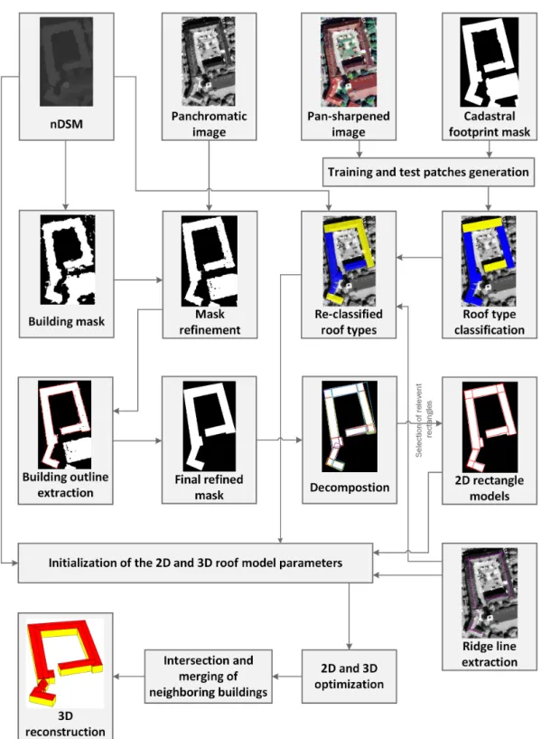
The method starts with the refinement of the DSM-based building masks and the simplification of the extracted building outlines. DSM data is integrated with high spatial resolution panchromatic images to improve building mask spatially in the boundaries area. Using the refined masks, a novel automatic method was developed for an optimized extraction and simplification of the building outlines. After extraction of the building outline, the building polygon is decomposed into the rectangular shapes using the line segments of the building outlines. After that, among generated rectangles, those that have maximum overlap with the building mask and have minimum overlap with each other are selected to cover the whole building area. Therefore, the complex building polygons are decomposed into basic rectangular shapes. Overlaps between neighboring rectangles are considered to reconstruct intersection parts of neighboring models (connecting roofs models) and, consequently, have a continuous 3-D model. The next step is to recognize the roof type in order to reconstruct the 3-D model of the buildings. Since the roof type is the most important component of a building to reconstruct its LoD2, accurate recognition of roof types provides helpful information for the reconstruction process. In this work, roof type recognition is considered as a supervised classification problem, where different roof type categories are introduced according to their visibility of geometrical structures in image and DSM. Additionally, due to the focus of the experiments, only existing roof types in Munich city area are considered. The training and test set are generated based on new semi-automatic methods for roof type classification. As a classifier, a new image-based method is proposed based on deep learning algorithms which uses the geometrical information of the building roofs in satellite images [20]. Later, the classification results are updated using selected rectangle shape and DSM in a Bayesian framework. The results from aforementioned data-driven steps are applied as pre-knowledge to initialize 3-D parametric roof models [19]. In the end, a modified brute force search is used separately in 2-D and 3-D to find the best fitted model to the DSM among all possible solutions. Finally, the reconstructed models of rectangles are assembled through an intersection and merging process to reconstruct watertight 3-D models of each building blocks. Figure1shows the workflow of the multi-stage hybrid method for 3-D building model reconstruction.
3.1. Parameterized Building Polygon Extraction
This section is an overview of the method for refining of DSM-based building masks and the extraction of the building polygons which are explained in detail in Reference [12]. The building masks are enhanced by applying the SVM classification method to the gradient features of their corresponding PAN image. The SIFT algorithm [14] is used to extract the primitive geometrical features which have efficiency to extract the linear geometrical structures (e.g., line and corner) and is robust against existing noise in panchromatic satellite image.
In order to extract a building’s polygon, the building boundary points are traced on its corresponding refined mask and a set of line segments is fitted to them. The obtained line segments are then regularized by finding the building’s main orientations. All the line segments are assigned to their appropriate main orientations, where they should be either parallel or perpendicular to their assigned main orientations. Since this orientation classification is performed globally for the whole building, the close orientation distance of the line segments within a class might be spatially far from each other. Therefore, a locality constraint is imposed on the class members and regroups the nonlocal members with the line segments in their neighborhood. As a next step, a novel approach is proposed based on least-squares adjustment to align the line segments. This approach considers the multiple orientations of each building, which yields a more accurate delineation of building polygons. As a final step, the aligned line segments are intersected and connected to each other, resulting in the building’s final polygon. This method is able to extract the building polygons very close to the buildings’ original edges, even for complex buildings (e.g., buildings with inner yards and multiple nonrectilinear main orientations).
Figure 1.Workflow of the 3-D building reconstruction. 3.2. Building Polygon Decomposition and Selection
The shape of resulting building polygons is usually complex and, thus, needs to be simplified. The main steps of this simplification are generalization, decomposition, and selection of the building polygon.
3.2.1. Generalization of the Building Polygons
The first step of the generalization is the simplification of the building outlines to reduce their vertices, while preserving the main shape of the building. A rule-based simplification is proposed to
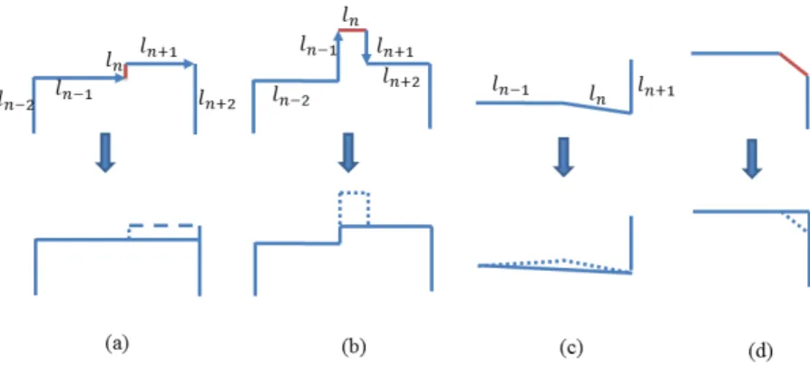
apply to the building polygons which discards short line segments. These rules are based on three cases introduced in Reference [65], and a modification is proposed in this paper in which several sequential lines with small differences angles are replaced with a single line. Figure2shows these simplification rules. Cadastral map-based footprints include adjacent buildings which mostly share common line segments. Before simplification of the footprints, the adjacent buildings are aggregated by removing the common line segments to generate a single building block which eases the simplification process and reduces the amount of data significantly. Common line segments are detected and discriminated from the outer part of the building outlines based on the gradient changes on the building mask. The last step of generalization is rectification in which the building polygons closer to rectangular shapes become totally rectangular and approximately collinear lines become one straight line.
Figure 2. Simplification rules: (a) Unidirected lines with a small offset ln, (b) extrusion, (c) approximately parallel lines, and (d) corners.
3.2.2. Decomposition of the Building Polygons
Since the common building shapes in urban areas are rectilinear, the generalized complex building polygons can be simplified to the several basic rectangle shapes in the decomposition step. In this paper, the decomposition is performed by creating a rectangle from each generalized line segment of the building polygon. Each line segment is moved by a step size of one pixel toward building masks iteratively until it meets a buffer of another parallel line segment of the building polygon or footprint. A rectangle is generated using these two parallel line segments. In Figure3, for instance, after moving the line segment several times (shown in blue), it lies in the buffer of another line segment of the building polygon (the yellow rectangle in Figure3).
Figure 3.Rectangle creation using a moving line segment (red: building polygon, blue: moving line segment, and yellow: buffer of line segment).
3.2.3. Selection of the Relevant Rectangles
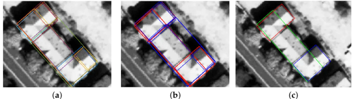
The rectangles generated usually overlap, and some of them are not representative enough for the building modeling. In Figure4b, for example, the blue rectangles are not good candidates for building modeling because a part of them is outside the building mask. Thus, a combination of the rectangles needs to be selected in which the rectangles have a minimum overlap with each other, cover the whole
building footprint, and represent the main part of the building. Two overlap tests are employed to identify the relevant rectangles. These tests are inspired by the work of Kada and Luo [66], in which the authors decomposed a footprint into several cells based on extending and intersecting the half-space planes. They further computed the overlap between the decomposed cells and the original footprint and compared it with a threshold to realize which cells are meaningful and belong to the building. In the proposed method, instead of using the decomposed cells, the relevant rectangles are selected by computing the overlap between rectangles and between every rectangle and the building mask. Thus, the rectangles are sorted based on the length of their related line segments, beginning with the rectangle with the longest line segment. The relevant rectangles are then selected by computing the percentage of the overlap of every rectangle with the building mask:
Overlap1=
Area(Maskrectangle∩Maskbuilding)
Area(Rectangle) >thr1. (1)
After selecting the first relevant rectangle based on Equation (1), the overlap of the other candidate rectangles with the relevant rectangle is measured. The rectangle with the largest overlap is selected as the relevant rectangle, which is then considered as a reference rectangle to compute its overlap with the other remaining candidate rectangles according to the following equation:
Overlap2=
Area(Rsearch∩Rre f erence)
Area(Rsearch) >thr2, (2)
whereRsearchis the candidate rectangle andRre f erenceis the relevant rectangle. The values of thresholds (i.e.,thr1andthr2) are changed based on the complexity of the area and dataset (cadastral map based
footprint or extracted building polygon). It turns out, based on empirical investigation, that the values ofthr1=thr2=0.8 are a good compromise. The final result of the rectangle selection process is shown
in Figure4c.
(a) (b) (c)
Figure 4.Rectangle-based decomposition: (a) Rectangle extraction based on building polygon line segments; (b) illustration of rectangles (blue: redundant rectangles, red: relevant rectangles); and (c) selected rectangles.
3.3. Roof Type Classification
In this section, the roof model type of each rectangle obtained from the previous steps is recognized in order to reconstruct the 3-D model of the roofs. An image-based method is proposed as a classifier based on deep learning algorithms which use the geometrical information of the building roofs in satellite images [20].
3.3.1. Building Roof Library Definition
A roof model library is necessary to define model-based 3-D building reconstruction. Since our experiments are focused on buildings in the city of Munich, we define our roof model library based on the most common roof types in this area. In addition, the resolution and quality of the DSM are
important criteria when selecting roof types for the library. Since a 3-D parametric roof model is reconstructed from the DSM of satellite imagery, the six roof types: Flat, gable, half-hip, hip, pyramid, and mansard roof models shown in Figure5create the roof model library based on their height and geometrical characteristics in the DSM and PS images.
3.3.2. Dataset Generation based on Roof Model Library
Training and test image patch datasets are generated from RGB channels of PS images with high spectral and spatial resolutions to classify the roof types and evaluate the results. The PS images are tiled into smaller patches based on the building mask skeleton points as each patch contains a whole or part of a roof type. The roofs are masked using building masks extracted from the footprint of the cadastral map to reduce the impact of their surrounding objects (e.g., trees and asphalt). Since cadastral map-based footprints are available and the refined building masks are very close to them, they are used for generating both training and test patches. Each patch is assigned to a label manually based on its corresponding roof type [20]. The main difference between this approach and previous image patch dataset generation approaches [67,68] is that the main orientation of each roof is also considered inside the patch. Therefore, the quality of roof patches cannot be degraded by rotation and resizing. The library of the roof patches is shown in Figure6based on the defined roof model library in Figure5.
(a) (b) (c) (d) (e) (f)
Figure 5. Roof model library (a) flat, (b) gable, (c) half-hip, (d) hip, (e), pyramid, and (f) mansard roof models.
Figure 6.The library of roof patches including six roof types.
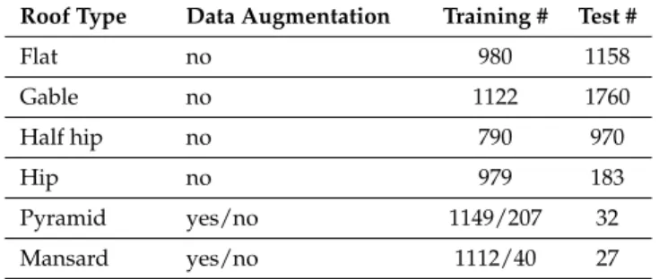
The number of instances of some roof classes is extremely low in comparison to other classes (such as mansard and pyramid roofs). Augmentation methods are used to increase the training patches of these roof types to deal with the small number of samples for the pyramid and mansard roofs and in order to balance the number of samples for all roof type categories. Converting to HSV color space, flipping the image to the right side, and rotation of 45◦are among several different augmentation methods in previous deep learning-based researches used in this paper. These augmentation methods can also increase the robustness of the results against rotation and color changes. The distribution of the training and test patches before and after augmentation are shown in Table1.
Table 1.The distribution of the training and test sets used in the experiment.
Roof Type Data Augmentation Training # Test #
Flat no 980 1158 Gable no 1122 1760 Half hip no 790 970 Hip no 979 183 Pyramid yes/no 1149/207 32 Mansard yes/no 1112/40 27 3.3.3. Deep Learning-Based Roof Type Classification
The convolutional neural networks (CNNs) can automatically learn structured and representative features through layer-to-layer hierarchical propagation schemes as high-level features learn from lower-level ones. The resulting features are invariant to rotation, occlusion, scale, and translation and are beneficial for the wide variety of object detection and classification tasks since they reduce the need for designing complicated engineered features [69,70]. The most published works in the computer vision field uses CNNs in four different manners: training the network from the scratch when there is a very large datasets available, fine-tuning the weights of an existing pretrained CNN when smaller dataset is accessible, using a pretrained CNN as a feature extractor to extract deep convolutional activation features (DeCAFs), and combining deep features and engineered features to train more powerful and accurate classifiers. The focus of our work is to apply second and third strategies (i.e., fine-tuning pretrained CNNs and applying SVM on the deep features) to classify roof types with a small dataset and then to select the one with the highest accuracy to further process.
For visual recognition tasks, different pretrained models for CNN networks, such as AlexNet [71], VGGNet [72], GoogleNet [73], and ResNet [74] have been trained on large datasets, such as ImageNet (1.2 M labeled images with 1000 categories). The VGGNet 16/19 and ResNet 50/101/152 have shown effective performances in the classification of remote sensing images [75,76] and are employed in our work for roof type classification.
The pretrained VGGNet is a deep network with a very simple structure. It contains 3×3 convolutions (i.e., conv layers) stacked on top of each other in increasing depth and 2×2 max pooling reducing the volume size all over the network. These layers are followed by three fully connected (FC) layers: The first two have 4096 nodes for each, and the third has 1000 nodes corresponding to the classes of ImageNet dataset. The fine-tuning of the new network starts with weight initialization of the last FC layer (i.e., FC8). All the other layers are then fine-tuned. For roof type classification, we add a new FC layer with six nodes to pretrained models for the classification of roofs into six categories. The networks are then fine-tuned on our dataset. The pretrained VGGNet as a feature extractor applied on all training and test patches to extract DeCAFs from the first two FC layers (i.e., FC6 and FC7). A conventional classifier such as SVM is then applied on DeCAFs to classify test patches. The VGG 16 (with 13 conv and 3 FC layers) and VGG 19 (with 16 conv and 3 FC layers) are very deep versions of VGGNet. These networks increase the classification performance due to having enriched features which are obtained by stacking deep layers.
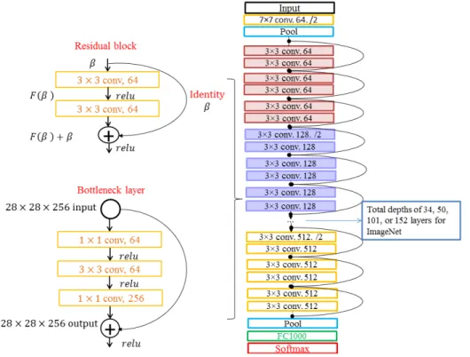
He et al. [74] showed that stacking deep layers in the plain networks deduce the classification performance due to vanishing gradient problems and a high number of parameters. They proposed a solution based on deep residual learning framework and accordingly developed very deep networks, the so-called ResNet. The residual block, as shown in the top left of Figure7, is the basic building block of the ResNet architecture to learn the residual function ofF(β)which is related to the standard function ofH(β) =F(β) +β.
The idealH(β)is learned by any model which is closer to identitying functionβthan random. Therefore, instead of having a network which learnsH(β)from randomly initialized weights, the residualF(β)is learned. This idea not only saves the training time but also solves the problem of the
vanishing gradient by allowing the gradients to pass unchanged through these skip connections [77]. In the architecture of the ResNet, as shown in Figure7, the stacked residual blocks are together with two 3×3 conv layers. The downsampling is performed directly by convolutional layers that have a stride of 2 [74]. Moreover, the ResNet model has an additional conv layer at the beginning and a global average pooling layer at the end after the last conv layer. It has an FC layer with 1000 neurons and a softmax [74]. Regarding the deeper ResNet 50/101/152, the stacked residual blocks have three conv layers in the bottleneck architectures, which lead to more efficient models [74].
For roof type classification through fine-tuning pretrained ResNet, similar to VGGNet, the last layer (i.e., FC1000) is replaced by a new FC layer with six classes corresponding to six roof types. For the second strategy, the DeCAFs are extracted from FC1000 for all training and test patches. The SVM classifier with a RBF kernel is then applied on the feature vectors which have 1000 dimensions to classify the roof types.
Figure 7.Residual block (top left), bottleneck layer (bottom left), and ResNet architectures (right). The aforementioned strategies for roof type classification have been performed in the Caffe framework [78]. The fine-tuned models and the trained SVM model are applied to the all four test datasets. In order to quantitatively evaluate the classification performance of the models, their results are compared to the ground truth [79], using a standard measure, such asQuality, which is calculated based on:
F1−score=
2×TP
2×TP+FN+FP (3)
In Equation (3),TP(True Positive) is the number of patches which belongs to the same class in the both test data and ground truth,FP(False Positive) is the number of patches from different classes which are classified wrongly as current test class,FN(False Negative) is the number of patches which are classified wrongly to the incorrect classes, andTN(True Negative) is the number of patches which do not belong to the same class in the test data and ground truth.
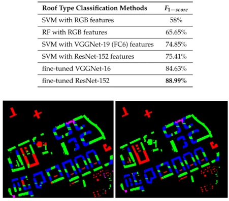
Based on the classification results as shown in Table2, the fine-tuned pretrained ResNet-152 outperform the other methods with theQualityof 88.99 %. The results of this method are then used as pre-knowledge in the next steps and updated later by fitting their models to the DSM data in the next step. Figure8illustrates the roof type classification result of the fine-tuned pretrained ResNet-152 for the second area.
Table 2. Comparison ofF1−scorefor the best results of DeCAFs, the best results of fine-tuned CNN models and conventional models, such as RF and SVM, with RGB features.
Roof Type Classification Methods F1−score
SVM with RGB features 58%
RF with RGB features 65.65%
SVM with VGGNet-19 (FC6) features 74.85%
SVM with ResNet-152 features 75.41%
fine-tuned VGGNet-16 84.63%
fine-tuned ResNet-152 88.99%
Figure 8.Illustration of classified roof types (left) and ground truth (right): gable (green), half-hip (blue), flat (red), hip (yellow), mansard (light blue), and pyramid (pink) roofs.
3.4. 3-D Building Reconstruction
In this step, a hybrid approach is proposed to reconstruct 3-D building models (LoD2) by utilizing the nDSM of satellite imagery and the results of the previous data-driven steps which initialize geometrical parameters of the roof models. The geometrical parameters obtained from building rectangles are further enhanced by computing height discontinuities from nDSM data and combination of the roof types. In addition, the roof type classification results are updated for each rectangle according to a set of roof combination rules and the nDSM data. The optimization is performed on the primary models obtained from the initial parameters to improve them and to have the best fit to height data and boundary of buildings.
3.4.1. Definition of Geometrical Structure of the Roof Model
The geometrical parameters of the primitives in the library are defined as follows:
ψ∈Ψ; Ψ={P,C,S }, (4) where the parameterΨcontains the position parametersP = {xo,yo,orientation}and the contour parametersC ={length,width}which are related to the rectangle. The shape parametersSincluding ridge/eave heightsZridge;Zeave; and the longitudinal and latitudinal hip distanceshipl1,hipl2,hipw1,
The roof components, such as vertices, edges, and planes are determined from the aforementioned parameters and their geometrical relationships [19,49] as shown in Figure9.
Figure 9.Geometrical parameters of the roof models.
3.4.2. Decomposition of the Rectangles Based on the Roof Types and Height Discontinuities
The rectangles can be enhanced by decomposing them based on considering some rules for a combination of the roof types obtained from the roof types classification step. A rectangle is decomposed where either a flat roof neighbors one of the sloped roofs or pyramid and mansard roofs neighbor other sloped and flat roof types. In Figure10a, for instance, a pyramid roof shown in magenta color is separated from the other roof type (i.e., gable roof with green color) by decomposing rectangles where a pyramid is changed to another roof type.
(a) (b)
Figure 10.Decomposition of a rectangle after imposing the rules of roof type combination: The pyramid roof is shown in magenta before (a) and after (b) the decomposition.
Furthermore, the rectangles can be enhanced by detecting height discontinuities. Since the basic shape of the model is rectilinear, the height discontinuities are measured on two height profiles of the middle lines. Each pixel on these two lines has different height values (Z) obtained from the nDSM. The gradient (G) is then computed as the profile derivative based on the predefined resolutionrs(here, rsis selected as one pixel):
∆Z ∆x(i) = Z(i+rs)−Z(i) rs = G(i) rs . (5)
Pixels with gradients (height differences) less than a threshold (threshold selected to be one meter) are then grouped to one class. Each class should contain more than four pixels; otherwise, it is not considered in computing height discontinuities. If the difference between the height averages of two sequential classes is more than a threshold (threshold selected to be 2 m), there is a height discontinuity point between them. The points with large gradients where the classes are separated are detected as the height discontinuity points. The points detected on the rectangle sides are then excluded. Finally, the rectangles are split at the positions of the height discontinuity points. Figure11
shows the result of height discontinuity detection for a building. As shown in Figure11c, there are two height discontinuities on the longitudinal profile of the rectangle.
(a) (b)
(c) (d)
Figure 11.Height discontinuity detection: (a) Longitudinal profile line (blue) and latitudinal profile line (red) drawn on the nDSM; (b) decomposition of the blue rectangle in Figure11a based on height discontinuity points (two magenta points in Figure11a); (c) the 3-D point clouds projected in the 2-D plane passing the longitudinal profile (red points); and (d) the 3-D point clouds drawn in the 2-D plane passing the latitudinal profile. The blue ellipses show the groups of points with height differences less than one meter.
3.4.3. Roof Type Classification Update
Image-based roof types classification results in some failures due to the small patch size which cannot cover a whole rectangle, especially in the case of long rectangles. Therefore, one rectangle can have either more than one roof type or only one incorrect roof type. To improve the roof type classification results, two strategies are suggested. Firstly, a set of combination rules is set up to assign only one roof type to each rectangle. For instance, a combination of gable with half-hip or hip roof is meaningful, which results in half-hip or hip roofs. Secondly, the height information from the nDSM is used to make a final decision on the roof type. In the first strategy, a rectangle is divided into three parts. A roof type is then assigned to each part based on the majority of pixels in each class. Next, a set of rules based on the combination of these roof types is determined as follows:
• {half-hip,gable,half-hip} or {half-hip,half-hip,hip} or {hip,half-hip,half-hip} or {hip,half-hip,hip}
−→{hip},
• {gable,half-hip,half-hip} or {gable,gable,half-hip} or {half-hip,gable,gable} or {half-hip,half-hip,gable}−→{half-hip},
• {gable,hip,gable}−→{hip}, and {gable}, • {gable,half-hip,gable}−→{gable},
In the second strategy, the image-based classification results are employed to compute the prior probabilities of each class. For this purpose, a table (Table3) including true positive and false negative
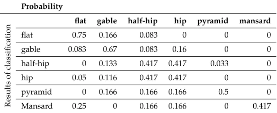
ratios of each roof type is computed based on the confusion matrix of the roof type classification results. In this table, the roof which is chosen from the classification takes the highest probability among other misclassified roof types. In the first row, for instance, the flat roof takes the highest probability, but the gable and half-hip roofs (as false negative roof types) also take a portion in the final decision of roof type selection. Table3only conducts the user to give probabilities to each type of roof and is useful in creating Table4. Since the classification results are obtained from a few small areas with a limited number of patches for some roof types such as pyramid and mansard roofs, it is not perfectly reliable to present the prior information about the roof types and to use for fusing with the nDSM. Therefore, the handcrafted probability is calculated for each roof type as a prior probability (Table4) according to the statistical information obtained from the roof type classification results (Table3). The prior probability of each roof type selected as multiple of the fraction of six (i.e., the number of roof types) and their sum is equal to 1. In the first row of Table4, for instance, we consider the probability of 4.5/6 = 0.75 for a flat roof, since the flat roof in the first row of confusion matrix (Table3) has a high true positive ratio. Since the false negative ratio of gable is 4 times more than half-hip roof, it may take a bigger portion than half-hip to be selected instead of flat roofs. Therefore, a 1/6 = 0.166 probability is given to gable roof and a 0.5/6 = 0.083 probability is given to half-hip roofs.
Based on this predefined probability, a Bayesian formulation is used to select the best roof type. The Bayesian approach is known to be robust and useful for parameter estimation problems. A set of modelsM={M1,M2, ...,Mm}for presenting dataDis given. Each model is presented by the prior
probabilityP(Mi)according to the probabilities shown in Table4.P(D|Mi)is the likelihood which is the probability of the observing dataDknowing the modelMi. Bayes’ rule states the following:
P(Mi|D) = P(D|Mi)P(Mi)
P(D) ∝P(D|Mi)P(Mi) (6)
where P(Mi|D) is the posterior probability for each roof type. P(D) is the normalizing constant which does not depend on the modelM; therefore, it is not considered in calculatingP(Mi|D)and an unnormalized density is preferred [80]. The best model ˆMiwith high posterior probability is then chosen from the entire set of possible solutionsM.
ˆ Mi=arg max Mi∈M (P(Mi|D)) =arg max Mi∈M {P(D|Mi)P(Mi)} (7)
Let us considerDias the partial data of rectanglei.P(D|Mi)is also shown as likelihoodL(Di|Mi), which is given by the inverse exponential function of weighted average of orthogonal Huber distance as the following equation:
L(Di|Mi)∝exp(− s 1 N
∑
j ρ(od 2 j)) (8)whereNis the number of inner nDSM pixels of the rectangle andρ(od2j)is the Huber loss [81], which is computed by
ρ(od2j) =
(1
2od2j for|odj|<T
T(|odj| −12T), otherwise (9)
In this equation,od2j is the shortest orthogonal distance (Euclidean distance) from 3-D pointpjobtained from nDSM to the surface of the 3-D model defined by configurationMiandTis the threshold of this error, which is computed by fitting a plane to the part of the nDSM of the building and by calculating the percentage of the points which have the closest distance to the surface of the 3-D model. This threshold is equal to 1 m.
The likelihood function is proposed based on Huber distance to down-weight the observation with large residuals and outliers. For this purpose, the orthogonal distance of the 3-D point clouds
to the fitted model are reweighed based on Huber distance. Therefore, the Root Mean Square Error (RMSE) is calculated based on the weighted average of residuals as a power of the exponential function which calculates the probability between 0 and 1.
Table 3.The confusion matrix of the classification for all four areas (Section3.3).
Flat Gable Half-hip Hip Pyramid Mansard
Flat 0.97 0.027 0.006 0 0 0 Gable 0.028 0.908 0.0028 0.066 0 0 Half-hip 0 0.094 0.81 0.0915 0 0.0045 Hip 0.006 0.056 0.087 0.85 0 0 Pyramid 0 0.144 0.36 0.12 0.38 0 Mansard 0.51 0 0.215 0.275 0 0
Table 4.Prior probabilities of roof models.
Probability
Results
of
classification
flat gable half-hip hip pyramid mansard
flat 0.75 0.166 0.083 0 0 0 gable 0.083 0.67 0.083 0.16 0 0 half-hip 0 0.133 0.417 0.417 0.033 0 hip 0.05 0.116 0.417 0.417 0 0 pyramid 0 0.166 0.166 0.166 0.5 0 Mansard 0.25 0 0.166 0.166 0 0.417 3.4.4. Initialization
The main orientation of the roof model is determined based on the ridge line orientation. Supposing the symmetry of a roof, the ridge line is one of the middle lines of the rectangle. To detect the ridge line of a rectangle, a buffer is considered around each middle line of a rectangle. The maximumZvalues are then computed for each orientation. The maximum value of each orientation is replaced by the mean of theZvalues of the neighboring pixels within a window size ofwidthrectangle/4 to reduce the noise effect of the DSM. After that, a threshold is defined according to the minimum value of these maximum values for each middle line. The number of points (NPoints) which haveZ values higher than this value is then determined for each orientation. If there is a significant difference between the number of points, the middle line and its orientation with the maximumNPointsis selected as the ridge line and main orientation of roof model. Otherwise, the main orientation of the roof model can be updated as well during updating roof types. The orientation with minimal error of the model fitting will be selected as the final main orientation. The height points of neighboring rectangles can affect the determination of the main orientation of each rectangle for complex buildings with several parts and orientations, where the rectangles overlap each other. Dealing with this issue, the height values of half of the overlapping pixels related to neighboring rectangles are lowered to the height of the rectangle’s border. The main orientation of the roof model is then computed according to what has been explained above. Figure12shows the result of roof model orientation detection for a U-shapebuilding.
Figure 12.Roof model orientation detection.
The position of the rectangle center (xoandyo) is calculated by averaging the four vertices of the rectangle. Thelengthandwidthof rectangles are replaced by each other regarding the orientation of the roof model. The ridge and eave heights are estimated based on averaging the pixels within two buffers, each with a different width around the ridge line and rectangle border, which is inspired by Reference [82].
The initialization of latitudinal and longitudinal hip distances, such ashipw1,hipw2,hipl1, and
hipl2, in Figure9is calculated based on the following geometrical rules:
• The initial value of longitudinal hip distance for the hip roof ishipl2=hipl1=length/3,hipl2=0,
andhipl1=length/3 for half hip roofs andhipl2=hipl1=0 for the gable roof.
• hipd1andhipd2are equal to the half the rectangle width for gable, half-hip, and hip roofs.
• The initial value of longitudinal hip distance for mansard roofs ishipl2=hipl1=length/3 and
hipd2=hipd1=width/3 for latitudinal hip distance.
• The initial value for a pyramid roof ishipl2=hipl1=length/2 andhipd2=hipd1=width/2.
The other important parameter for fitting the 3-D model to the nDSM is the determination of the hip part in the half-hip roof. Since the roof type classification only determines the roof types without giving the results about their geometrical structures, the hip part of half-hip roof is an unknown parameter. This parameter is determined based on the comparison of the height computed in the small buffer at the end of the ridge line. Therefore, the side with the smaller height value is selected as ahipside.
3.4.5. Optimization
In this section, the complete parametric roof model is reconstructed precisely by an optimization method. The optimization is performed for 2-D and 3-D parameters in sequence based on a brute-force algorithm which discovers the best combination among all combination of the parameters. All possible models are generated by changing the parameters in the predefined ranges. The range of refinement of the model parameters is limited since the initialization is acceptable in most of the buildings. Table5represents the range of each parameter and their corresponding step sizes. The ranges are selected experimentally as a compromise between the accuracy and computational time. An increase in parameter range could result in an exponential growth in the computational time which can be an issue in the modeling of large-scale areas. It worth noting that the optimization process can be parallelized, allowing to search in a larger range of parameters. The same ranges of parameters have been defined for all four areas. We select the step size based on the resolution of DSM and PAN image (0.5 m). In the Z direction, the range is defined as two times of the uncertainty of the calculated eave/ridge heights, which is about 1 m. Hip distances are changed by changing the height values of ridge and eave lines. Since the height values are changed in the step size of 0.2 m, the hip distances change in sub-pixels. Therefore, the step size of hip distances is chosen as 0.16 m. In 2-D, the range of the center position of the polygon was defined as three pixels and the length and width of the rectangle were defined as five pixels to overcome the occlusion problems cause by adjacent trees to the building roofs.
Table 5.Predefined parameters and their corresponding ranges, units, and step sizes.
Parameters Ranges Unit Step Size
xo [−3, 3] pixel 1 yo [−3, 3] pixel 1 Zridge [−2.4, 2.4] meter 0.2 Zeave [−2.4, 2.4] meter 0.2 length [−5, 5] meter 1 width [−5, 5] meter 1 Orientation [−∆θ,+∆θ] degree 1
hipl1 [−1, 0.35]×initial(hipl1) meter 0.16
hipl2 [−1, 0.35]×initial(hipl1) meter 0.16
hipd1 width/2 meter 0
hipd2 width/2 meter 0
To reconstruct 3-D building model of one block of building including several roof models, the interaction between rectangles should be considered. The neighboring and overlapping rectangles are found to verify the interaction between models (rectangles) of a building block. In order to distinguish the two types of overlaps, the overlapping rectangles share a significant area which can be represented by an intersection roof model type, such asL-shapeorT-shape. The neighboring rectangles, however, share a small area which is not significant and cannot present a connecting roof model type. Figure13
shows the overlapping and neighboring rectangles.
Figure 13. Overlapping (red dots) and neighboring (green dots) parts of rectangles in one building block.
The workflow of 2-D optimization steps are shown in Figure14. The optimization is carried out through an exhaustive search in which all possible 2-D building models are generated by changing the initial 2-D parameters ofΨ1×11({xo,yo,length,width,orientation}) within the predefined ranges as
shown in Table5. The parameter combinations are then derived, and their model costs are calculated based on the Polygon and Line Segment (PoLiS) metric [83] between the model vertices and the reference building boundaries (extracted from the RANSAC fitting line to the building boundary points obtained from the PAN image and building mask). The PoLiS metric was proposed for measuring the similarity of any two polygons, which is a positive-definite and symmetric function satisfying the triangle inequality [83]. It changes linearly with respect to small translation, rotation, and scale changes between the two polygons. It takes into account the positional accuracy and shape differences between the polygons.
The PoLiS distance between the two polygons is computed as the summation of the two average distances. Letvj ∈V, j={1, ...,J}in each vertex ofVandu∈∂Ube its closed point (not necessarily a vertex) on the polygonU. The average distance betweenvjanduis then a directed PoLiS distance
~
dp(V,U)between polygonsV andUand is defined as
~ dp(V,U) =1 Jv
∑
j∈V min u∈∂Ukvj−uk. (10)Since the directed PoLiS distance~dpis made symmetrically, PoLiS metric is defined by summing and normalizing the directed distances as a relationship as follows:
~ dp(V,U) = 1 2Jv
∑
j∈V min u∈∂Ukvj−uk+ 1 2Ku∑
k∈U min v∈∂Vkuk−vk. (11)The best 2-D building model with the minimum cost is then selected for each rectangle. For the building blocks composing of more than one rectangle, the rectangles are ordered based on their lengths. After selecting the best model of the first rectangle (i.e., Ri and IndexR == 1), the best model for the second rectangle is selected by investigating its neighborhood relations with the other rectangles. If the second rectangle (Rj), for example, is adjacent to the first rectangle (i.e.,Ri ./Rj), the differences between the orientation of the first rectangle and the orientations of all possible models for the second rectangle are calculated. If these differences are within the angle threshold of [0, 90, 180, 270, 360]±(thrθ =15)(i.e., (θi−θj)< thrθ), the 2-D model with minimum cost and the minimum orientation difference is selected as the best 2-D model for the second rectangle; otherwise, the model with the minimum cost value is selected as the final model for the second rectangle. This method is used for selecting the best models for all rectangles in the building block.
Figure 14.2-D optimization workflow.
Figure15 shows the result of 2-D optimization used as input for 3-D optimization. In the vector of Ψ1×11, 3-D parameters are variable values and are optimized in combination with 2-D
parameters. The optimization algorithm is carried out based on an exhaustive search which is used for generating all possible 3-D building models by changing the initial values of the 3-D parameters (Ψ3−D = {zeave,zridge,hipl1}) in ranges defined in Table5. The cost values of each 3-D model are
calculated based on the RMSE of orthogonal Huber distances between the 3-D point clouds obtained from nDSM and the 3-D models. The best 3-D models with minimum cost are selected among all possible 3-D building models generated. Similar to the 2-D optimization, in a building block containing multiple rectangles, the relationships between the neighboring rectangles affect the model selection. By contrast, in the selection of the best 3-D building model, the height differences between ridge and eave lines of the neighboring rectangles are considered instead of orientation. The best 3-D model of the first rectangle is initially selected based on the minimum cost value. If the second model, for example, is neighbor to the first model (i.e.,Mi./Mj), the differences between the ridge/eave height values of all possible 3-D models of the second rectangle and best 3-D model of the first rectangle are calculated. If these differences are in a height threshold (thrh = 1 m) and in a cost threshold (thrcost = 1.5 m) (i.e.,∆Hridgeij)<thrh&∆Heaveij)<thrh&Costj<thrcost), the model with the minimum cost value and minimum height differences is selected as the final model for the second rectangle; otherwise, the model with the minimum cost value is selected. This method is performed for all rectangles in a building block.
Figure 15.3-D optimization workflow. 3.4.6. Intersection and Reconstruction
The models for the parts created are intersected with each other to reconstruct the 3-D building model for one building block including several parts. Different connecting roof types, such asL-shape, T-shape, andPlus-shape, can be further created. Depending on the type of interaction between the models (the degree of overlap), the roof type of neighboring models, and the minimum cost value, the proper connecting roof type is chosen. Neighboring models which have significant overlap create different connecting roof models. Figure16a shows the different models and their related connecting roof models. The intersection points of two basic mansard models which overlap each other are computed to create several connecting roof models, as Figure16b shows. For example,
Mansard roof models, as a complete roof type including eleven parameters, are extensible to other roof models defined in the library with fewer parameters. After creating different connecting roof models, the one with the least cost value (Equation (9)) is selected. If the cost values are close, theL-shapeis selected which is simpler with fewer intersection points.
(a) 𝑎10 𝑎16 𝑎1 𝑎2 𝑎3 𝑎4 𝑎 5 𝑎6 𝑎7 𝑎8 𝑎9 𝑎11 𝑎12 𝑎13 𝑎14 𝑎15 𝑎17 𝑎18 𝑎19 𝑎20 𝑎22 𝑎21 𝑎24 𝑎23 𝑓1 𝑓2 𝑓3 𝑓4 𝑓5 𝑓10 𝑓6 𝑓7 𝑓8 𝑓9 𝑓11 𝑓12 𝑓13 (b)
Figure 16.(a) Connecting roof types and (b) possible connecting roof types by different combinations of the roof vertices and intersection points (green points) of the two mansard roofs
4. Experiments
In order to evaluate the proposed approach, the 3-D building models of four different areas in Munich are reconstructed and the results are evaluated qualitatively and quantitatively, comparing with LiDAR data as the reference.
4.1. Data Description
4.1.1. Stereo Satellite-Based DSM and Images
The experimental datasets for this research work consist of PAN images with resolutions of 0.5 m, multispectral images with resolution of 2 m (8 channels) captured by WorldView-2 satellite imagery from Munich, and the corresponding pansharpened and stereo satellite-based DSMs with resolutions of 0.5 m. WorldView-2 is one of the VHR satellite sensors which is used with along track stereoscopy technology. Using along track stereoscopy technology, this sensor can acquire two stereo pairs in a large area on the same day and same orbit with an overlap in the test area, leading to four views with stereo angles between 12◦and 24◦[3,84]. DSMs of the stereo pair are generated using semi-global matching (SGM) [85] for dense image matching [6]. The nDSM exhibits the heights of objects above the ground, which can be simply described as subtraction of the DTM from DSM. For this research work, the DTM is generated from DSM based on an advanced morphological method in which low rank median and high rank median filters are applied, respectively [27].
4.1.2. LiDAR Based DSM
The DSM of LiDAR data is used for the evaluation of the 3-D building reconstruction results. In order to generate the DSM, the first pulse of LiDAR data including the ground and objects above-ground, such as trees and buildings, is rasterized at a resolution of 0.5 m after coordinate system transformation. After that, B-Spline interpolation is used to generate the DSM. The LiDAR data is captured by airborne LiDAR which detects the terrain surface from the aircraft. The data is provided by the “State Office for Digitization, Broadband and Surveying” of Munich. The resolution of the data is 5 points/m2.
4.1.3. Building Mask
For building detection and mask generation, the data-driven approach proposed by Reference [27] is used. This approach is able to generate building masks fast and fully automatic. The ground level and elevated objects are firstly discriminated using the nDSM data of VHR satellite imagery. The buildings were then extracted from the surrounding patterns and clutters based on advanced rule-based fuzzy spectral classification on PS VHR satellite images (WorldView-2) followed by a height thresholding (i.e., 2 m).
4.2. Qualitative Evaluation
Visualizations of 3-D building models and their proximities to the building structures in reality are major criteria for evaluating 3-D model reconstruction approaches in technical applications. Figures17–20show the results of our proposed approach, where the results of the outline extraction and decomposition, height discontinuity detection, roof type classification, ridge line orientation identification, and 3-D building model reconstruction are illustrated in the sub-figures (a–f), respectively. As shown in these figures, the proposed algorithm can reconstruct the high-rise buildings (more than 3 m in height) and the buildings with average areas larger than 75 m2(300 pixels with a resolution of 0.5 m). The low-rise and small structures, such as garages, were discarded due to the thresholds used in the building detection step. A total number of 208 buildings, including single, compound, and complex buildings with inner yards, multiple orientation, or multiple roof types, were reconstructed. According to the results, the 3-D building model reconstructions were satisfactory, except for a few buildings.
Figures21and22illustrate examples of the reconstructed building models. More precisely, the height discontinuities were detected correctly in B0, B3, and B8. Moreover, the 2-D quadrilateral footprints demonstrate the successful intersection of neighboring rectangles to fit the building shapes. Moreover, B7 shows the strength of our approach in reconstructing buildings with multiple roof types, such as the half-hip and pyramid roofs in this example. Further examples of buildings with multiple roof types can be seen in B5 and B8 with flat-slopped and hip-mansard roofs, respectively. In addition, B4 shows that our proposed approach can intersect both perpendicular and parallel rectangles.
In addition to its strengths, our proposed approach suffers from a few drawbacks. There are some buildings in which the height discontinuities are under- or over-detected due to the poor quality of the DSM data. The over-detection of height discontinuities could cause the rectangle to be over-split, as depicted in B9. Our approach assumes rectilinear forms as the basic building shapes similar to the typical forms of the building footprints in urban areas. However, there are buildings with nonrectilinear shapes, such as the one depicted in B8. Moreover, some remarkable roof types, such as conical, shell, semi-ellipsoid, elliptic, and spherical, which have been not predefined in the library, are reconstructed based on existing roof types in the library. In B6, for example, the semi-ellipsoid-shaped roof was reconstructed by some flat roof shapes at different height levels due to gradual elevation changes. Furthermore, the cylindrical tower with a conical roof in B8 was reconstructed as a cubic structure with a hip roof. The intersection can suffer deficiencies if the intersection rule is not defined for different roof types. The failure case because of decomposition is shown in B6, where the building is divided into too many rectangles, while the building seems to be covered only by one rectangle.
(a) (b)
(c) (d)
(e) (f)
Figure 17.Illustration of the preprocessing steps of 3-D building model reconstruction for the first area (Area-1): (a) Decomposed 2-D building outline into rectilinear shape, (b) detected height discontinuities (green lines), (c) classified roof types (red: flat, green: gable, blue: half-hip, yellow: hip, magenta: pyramid, and cyan: mansard) and (d) extracted ridge lines (blue lines), (e) 3-D building models on the PAN image, and (f) 3-D building models.
(a) (b)
(c) (d)
(e) (f)
Figure 18. Illustration of the preprocessing steps of 3-D building model reconstruction for the second area (Area-2): (a) Decomposed 2-D building outline into rectilinear shape, (b) detected height discontinuities (green lines), (c) classified roof types (red: flat, green: gable, blue: half-hip, yellow: hip, magenta: pyramid, and cyan: mansard), (d) extracted ridge lines (blue lines), (e) 3-D building models on the PAN image, and (f) 3-D building models
(a) (b)
(c) (d)
(e)
(f)
Figure 19.Illustration of the preprocessing steps of 3-D building model reconstruction for the third area (Area-3): (a) Decomposed 2-D building outline into rectilinear shape, (b) detected height discontinuities (green lines), (c) classified roof types (red: flat, green: gable, blue: half-hip, yellow: hip, magenta: pyramid, and cyan: mansard), (d) extracted ridge lines (blue lines), (e) 3-D building models on the PAN image, and (f) 3-D building models.
(a) (b)
(c) (d)
(e) (f)
Figure 20. Illustration of the preprocessing steps of 3-D building model reconstruction for the fourth area (Area-4): (a) Decomposed 2-D building outline into rectilinear shape, (b) detected height discontinuities (green lines), (c) classified roof types (red: flat, green: gable, blue: half-hip, yellow: hip, magenta: pyramid, and cyan: mansard), (d) extracted ridge lines (blue lines), (e) 3-D building models on the PAN image, and (f) 3-D building models.
B0 B1 B2 B3 B4 B5 B6
Figure 21.Cont(Different examples of 3-D building models: PAN image (1st column), LiDAR data (2nd column), rectangles (3rd column), and 3-D building model (4th column)).