Deep unsupervised clustering with Gaussian mixture variational autoencoders

(1)

D

EEP

U

NSUPERVISED

C

LUSTERING WITH

G

AUSSIAN

M

IXTURE

V

ARIATIONAL

A

UTOENCODERS

Nat Dilokthanakul1,∗, Pedro A. M. Mediano1, Marta Garnelo1,

Matthew C. H. Lee1, Hugh Salimbeni1, Kai Arulkumaran2& Murray Shanahan1 1_{Department of Computing,}2_{Department of Bioengineering}

Imperial College London London, UK

∗_{[email protected]}

ABSTRACT

We study a variant of the variational autoencoder model with a Gaussian mix-ture as a prior distribution, with the goal of performing unsupervised cluster-ing through deep generative models. We observe that the standard variational approach in these models is unsuited for unsupervised clustering, and mitigate this problem by leveraging a principled information-theoretic regularisation term known asconsistency violation. Adding this term to the standard variational opti-misation objective yields networks with both meaningful internal representations and well-defined clusters. We demonstrate the performance of this scheme on synthetic data, MNIST and SVHN, showing that the obtained clusters are distinct, interpretable and result in achieving higher performance on unsupervised cluster-ing classification than previous approaches.

1 INTRODUCTION

Unsupervised clustering remains a fundamental challenge in machine learning research. While long-established methods such ask-means and Gaussian mixture models (GMMs) (Bishop, 2006) still lie at the core of numerous applications (Aggarwal & Reddy, 2013), their similarity measures are lim-ited to local relations in the data space and are thus unable to capture hidden, hierarchical dependen-cies in latent spaces. Alternatively, deep generative models can encode rich latent structures. While they are not often applieddirectlyto unsupervised clustering problems, they can be used for dimen-sionality reduction, with classical clustering techniques applied to the resulting low-dimensional space (Xie et al., 2015). This is an unsatisfactory approach as the assumptions underlying the di-mensionality reduction are generally independent of the assumptions of the clustering techniques. Deep generative models try to estimate the density of observed data under some assumptions about the latent structures, i.e., hidden causes. They allow us to reason about data in more complex ways than a general input-output mapping scheme. However, inference in models with complicated latent structures can be difficult. Recent breakthroughs in approximate inference have provided tools for constructing tractable inference algorithms. As a result of combining differentiable methods with variational inference, it is possible to scale up inference to datasets of sizes that would not have been possible with earlier inference methods (Rezende et al., 2014). One popular algorithm under this framework is the variational autoencoder (VAE) (Kingma & Welling, 2013).

In this paper, we propose an algorithm to perform unsupervised clustering within the VAE frame-work. To do so we postulate that generative models can be tuned for unsupervised clustering by making the assumption that the observed data is generated from a multimodal prior distribution, and construct a recognition network with a Gaussian mixture prior that can be directly optimised using the reparameterization trick. We also show that in the VAE framework, the standard mean-field ap-proximation used is not suitable for clustering, and can be mitigated with an information theoretic regularisation term known as consistency violation.

(2)

1.1 RELATEDWORK

Unsupervised clustering can be considered a subset of the problem of disentangling latent variables, which aims to find structure in the latent space in an unsupervised manner. Recent efforts have moved towards training models with disentangled latent variables corresponding to different factors of variation in the data. Inspired by the learning pressure in the ventral visual stream, Higgins et al. (2016) were able to extract disentangled features from images by adding a regularisation coefficient to the lower bound of the VAE. As with VAEs, there is also effort going into obtaining disentangled features from generative adversarial networks (GANs) (Goodfellow et al., 2014). This has been re-cently achieved with InfoGANs (Chen et al., 2016), where structured latent variables are included as part of the noise vector, and the mutual information between these latent variables and the gen-erator distribution is then maximised as a mini-max game between the two networks. Similarly, Tagger (Greff et al., 2016), which combines iterative amortized grouping and ladder networks, aims to perceptually group objects in images by iteratively denoising its inputs and assigning parts of the reconstruction to different groups.

The work that is most closely related to ours would be the stacked generative semi-supervised model (M1+M2) by Kingma et al. (2014). One of the main differences is the fact that their prior distri-bution is a neural network transformation of both continuous and discrete variables, with Gaussian and categorical priors respectively. The prior for our model, on the other hand, is a neural network transformation of Gaussian variables which parametrise the means and variances of a mixture of Gaussians, with categorical variables for the mixture components. As such, the categorical variables from Kingma et al. (2014) are additional inputs to a neural network mapping, whereas our model uses categorical variables as mixture components. Furthermore, we introduce a regularizer to im-prove unsupervised clustering performance. Crucially, Kingma et al. (2014) apply their model to semi-supervised classification tasks, whereas we focus on unsupervised clustering. Therefore, our inference algorithm is more specific to the latter.

We compare our results against several orthogonal state-of-the-art techniques in unsupervised clus-tering with deep generative models: deep embedded clusclus-tering (DEC) (Xie et al., 2015), adversarial autoencoders (AAEs) (Makhzani et al., 2015) and CatGANs (Springenberg, 2015).

2 VARIATIONAL

AUTOENCODERS

VAEs are the result of combining variational Bayesian methods with the flexibility and scalability provided by neural networks (Kingma & Welling, 2013; Rezende et al., 2014). Using variational in-ference it is possible to turn intractable inin-ference problems into optimisation problems (Wainwright & Jordan, 2008), and thus expand the set of available tools for inference to include optimisation techniques as well. Despite this, a key limitation of classical variational inference is the need for the likelihood and the prior to be conjugate in order for most problems to be tractably optimised, which in turn can limit the applicability of such algorithms. Variational autoencoders introduce the use of neural networks to output the conditional posterior (Kingma & Welling, 2013) and thus al-low the variational inference objective to be tractably optimised via stochastic gradient descent and standard backpropagation. In addition, a technique known as the reparametrisation trick has been proposed to enable backpropagation through continuous stochastic variables. While under normal circumstances backpropagation through stochastic variables would not be possible without Monte Carlo methods, this is bypassed by constructing the latent variables with a deterministic function and a separate source of noise. We refer the reader to Kingma & Welling (2013) for more details.

3 GAUSSIAN

MIXTURE

VARIATIONAL

AUTOENCODERS

In regular VAEs, the prior over the latent variables is commonly an isotropic Gaussian. This choice of prior causes each dimension of the multivariate Gaussian to be pushed towards learning a separate continuous factor of variation from the data, which can result in learned representations that are structured and disentangled. While this allows for more interpretable latent variables (Higgins et al., 2016), the Gaussian prior is limited because the learnt representation can only be unimodal and does not allow for more complex representations. As a result, numerous extensions to the VAE have been

(3)

developed, where more complicated latent representations can be learned by specifying increasingly complex priors (Chung et al., 2015; Gregor et al., 2015; Eslami et al., 2016).

In this paper we choose a mixture of Gaussians as our prior, as it is an intuitive extension of the uni-modal Gaussian prior. If we assume that the observed data is generated from a mixture of Gaussians, inferring the class of a data point is equivalent to inferring which mode of the latent distribution the data point was generated from. While this gives us the possibility to segregate our latent space into distinct classes, inference in this model is non-trivial. It is well known that the reparametrisation trick which is generally used for VAEs cannot be directly applied to discrete variables. One possi-bility for estimating the gradient of discrete variables is to calculate the likelihood ratio estimator using Monte Carlo sampling; however, this is known to have high variance (Eslami et al., 2016). Instead, we show that by adjusting the architecture of the standard VAE, our estimator of the vari-ational lower bound of our Gaussian mixture varivari-ational autoencoder (GMVAE) can be optimised without having to sample directly from the discrete distribution.

3.1 GENERATIVEMODEL ANDVARIATIONALINFERENCEMODEL

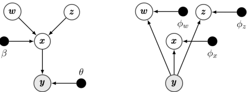
Consider the generative modelpβ,θ(yyy, xxx, www, zzz) = p(www)p(zzz)pβ(xxx|www, zzz)pθ(yyy|xxx), where an observed sampleyyyis generated from a set of latent variablesxxx,wwwandzzzunder the following process:

w ww∼ N(0, III) (1a) zzz∼M ult(πππ) (1b) x xx|zzz, www∼ K Y k=1 N µµµzk(www;β), diag σσσ 2 zk(www;β) zk (1c) yyy|xxx∼ N µµµ(xxx;θ), diag σσσ2₍_x_x_x_;_θ₎ orB(µµµ(xxx;θ)). (1d) whereKis a predefined number of components in the mixture, andµµµzk(·;β), σσσ

2

zk(·;β), µµµ(·;θ), and

σσσ2₍_·_;_θ₎_{are given by neural networks with parameters}_β _and_θ_{, respectively. That is, the observed} sampleyyyis generated from a neural network observation model parametrised byθand continuous latent variablexxx. Furthermore, the distribution ofxxxis a GMM with means and variances specified by another neural network model parametrised byβand with inputwww.

More specifically, the neural networkβoutputs a set ofKmeansµµµzkandKvariancesσσσ

2

zkwithwwwas

input. A one-hot vectorzzzis sampled from the mixing probabilityπππwhich chooses one component from the GMM. We set the prior parameterπππto the uniform distributionπk =K−1. The generative and variational views of this model are depicted in Fig. 1.

x

w

zzz

yyy

β

θ

x

w

zzz

yyy

φ

w

φ

x

φ

z

Figure 1: Graphical models for the Gaussian mixture variational autoencoder (GMVAE) showing the generative model (left) and the variational family (right).

3.2 INFERENCE WITHRECOGNITIONNETWORKS

The generative model is trained with the variational inference objective, i.e. the log-evidence lower bound (ELBO), which can be written as

LELBO=Eq _p β,θ(yyy, xxx, www, zzz) q(xxx, www, zzz|yyy) . (2) 3

(4)

We assume the mean-field variational familyq(xxx, www, zzz|yyy)as a proxy to the posterior which factorises asq(xxx, www, zzz|yyy) =Q

iqφx(xxxi|yyyi)qφw(wwwi|yyyi)qφz(zzzi|yyyi), whereiindexes over data points. To simplify

further notation, we will dropiand consider one data point at a time. We parametrise each variational factor with the recognition networksφx,φw andφz that output the parameters of the variational distributions. We specify the form ofqφx(xxx|yyy)andqφw(www|yyy)to be Gaussian posteriors. qφz(zzz|yyy)

has the form of a multinomial distribution. The lower bound can then be written as,

LELBO =Eq(xxx|yyy) logpθ(yyy|xxx)−Eq(www|yyy)q(zzz|yyy) KL(qφx(xxx|yyy)||pβ(xxx|www, zzz)) −KL(qφw(www|yyy)||p(www))−ηKL(qφz(zzz|yyy)||p(zzz)). (3)

We refer to the terms in the lower bound as the reconstruction term, conditional prior term,w-prior term andz-prior term respectively. We introduceη as a hyperparameter which adjusts the strength of thez-prior. We will discuss this term in more detail in sections 3.2.2 and 4.1.

3.2.1 THECONDITIONALPRIORTERM

The reconstruction term can be estimated by drawing Monte-Carlo samples fromq(xxx|yyy), where the gradient can be backpropagated with the standard reparameterisation trick (Kingma & Welling, 2013).wwwandzzzprior terms can be calculated analytically.

Importantly, by constructing the model this way, the conditional prior term can be estimated using equation 4 without the need to sample from the discrete distributionq(zzz).

Eq(www|yyy)q(zzz|yyy) h KL qφx(xxx|yyy)||pβ(xxx|www, zzz) i ≈ K X k=1 qφz(zk = 1|yyy) 1 M M X j=1 KLqφx(xxx|yyy)||pβ(xxx|www (j)_{, z} k= 1) (4)

Sinceqφz(zzz|yyy)can be taken directly from the output of the recognition network, the expectation

overqφz(zzz|yyy)can be calculated straightforwardly and backpropagated as usual. The expectation

overqφw(www|yyy)can be estimated withMMonte Carlo samples and gradients can be backpropagated

via the reparameterisation trick.

3.2.2 MEAN-FIELD APPROXIMATION AND CLUSTERING

In variational optimisation settings, a mean-field approximation is usually a good compromise be-tween tractability and performance. In our GMVAE clustering setting, however, thez-prior term in the ELBO costKL(qφz(zzz|yyy)||p(zzz))is problematic and results in poor clustering. The source of this

problem lies in the assumption of independence between observations.

Using exact inference, thez-prior term would force the system to produce a uniform label distribu-tion over the whole dataset – i.e. to assign the same number of samples to each classon average.1 However, under the mean-field approximation, this constraint is enforced oneach sample, and min-imising the KL divergence betweenqφz(zzz|yyy)and the uniform priorp(zzz)will force the label

distri-bution of each sample to be close to the uniform distridistri-bution. In this scenario there is no notion of clustering or multimodal latent space, and thez-prior becomes essentially an anti-clustering term. Empirically, as illustrated in Section 4.1, this term encourages the density mixture to become degen-erate, with the means and variances of all components converging to very similar values. This is a very undesirable scenario. To experiment with the interplay between this term and the information-theoretic regularisation introduced below, we introduce an ad-hoc tuning parameterηthat we use to adjust the strength of thez-prior term.

It is worth noting that this problem is not present in the structured VAE of Johnson et al. (2016). Unlike us, they use neural networks in some, but not all, parts of the inference model. This allows them to circumvent the problem by not making the independence assumption and using stochastic variational inference. One shortcoming of this approach is that during evaluation inferring the label of a sample is more expensive, as there is no explicit classifier network analogous to ourqφz(zzz|yyy).

1

(5)

3.3 INFORMATIONTHEORETICREGULARISATION WITHCONSISTENCYVIOLATION

It has been consistently observed that hidden stochastic layers in VAEs are hard to optimise. A common issue is that the higher layers are not fully utilised because they collapse early on in training before they are able to learn a useful representation. One way to mitigate this problem, suggested by Sønderby et al. (2016), is to gradually turn on the prior terms in Eq. (3). In this paper we adopt a different, more principled approach based on information theory (Cover & Thomas, 2006) and adapted from Ver Steeg et al. (2014). In short, we introduce an information-theoretic regularisation term to ensure that our discrete latent variables learn a meaningful representation.

According to Ver Steeg et al. (2014), a good clustering must satisfy what in information theory is known asconsistency under coarse-graining– i.e. any measure of uncertainty should not increase if the data is grouped together into clusters. Interestingly, it is possible to quantify precisely to what extent a proposed cluster assignment violates this condition. In a “shallow” clustering setting, with

Z being the cluster labels andXthe observed variables, thisconsistency violation(CV) is defined as

CV = ˆH(Z|X), (5) whereHˆ is an empirical estimator of conditional entropy from observed data. Although seemingly simple, CV has a very strong theoretical underpinning. In this setting, CV is merely the entropy of the labels given the visible variables. Intuitively, CV is minimised if each data point belongs unequivocally to one cluster, and is far from the borders of any other cluster.

In our deep clustering framework, however, it is not so clear how to apply this consistency condi-tion. For example, it could be applied to the observed variablesHˆ(Z|Y)or to the latent variables

ˆ

H(Z|X). To bypass this conundrum, we note that there is no reason to expect the data to be nat-urally clustered inyyy-space – if that were the case there would be no need for an encoding network or a VAE at all. Instead, it is more sensible to require that the latent representation of the data is properly clustered and well-defined. For this reason we add to our cost function a regularising term that corresponds to the consistency violation of the latent variables.

With this theoretical framework, we now face the problem of estimatingHˆ. In their original paper, Ver Steeg et al. use nonparametric nearest-neighbour estimators forHˆ in an attempt to avoid any assumptions aboutp(xxx). In our case, however, we have reason to follow a different approach. Since the generative mechanism assumes thatxxxis GMM-distributed, we will use this same assumption to estimate CV. This also entails that the CV cost remains differentiable, and can therefore be optimised using standard backpropagation.

With the considerations above, we estimate the consistency violation of the latent variablesxxx,wwwand the clustering labelzzzas

By incorporating this information-theoretic term to the lower bound, our full optimisation objective becomes

(6)

whereαis a trade-off hyperparameter that specifies the relative strength of the information-theoretic regularisation. Note that by embedding CV into this deep GMM clustering setting we have provided a principled way of optimising the partition of the data, an issue which was only preliminarily explored in Ver Steeg et al. (2014).

4 EXPERIMENTS

The main objective of our experiments is not only to evaluate the accuracy of our proposed model, but also to understand the interplay between the different factors involved in the construction of meaningful, differentiated latent representations of the data. This section is divided in three parts:

1. We first study the inference process in a low-dimensional synthetic dataset, and focus in particular on how the relative strengths of the different terms inLaffect the final result; 2. We then evaluate our model on an MNIST unsupervised clustering task; and

3. We finally show the generated images from the model conditioned on different values of the latent variables, which illustrate that the model can learn interpretable latent representation. Throughout this section we make use of the following datasets:

• Synthetic data: We create a synthetic dataset mimicking the presentation of Johnson et al. (2016), which is a 2D dataset with 10,000 data points created from the arcs of 5 circles.

• MNIST: The standard handwritten digits dataset, composed of 28x28 grayscale images and consisting of 60,000 training samples and 10,000 testing samples (LeCun et al., 1998).

• SVHN: A collection of 32x32 images of house numbers (Netzer et al., 2011). We use the cropped version of the standard and the extra training sets, adding up to a total of approximately 600,000 images.

4.1 SYNTHETIC DATA

First, we study the contribution of the different clustering-related costs in Eq. (7) in a simple 2D synthetic dataset. The dataset consists of 10,000 points, distributed in 5 distinct non-Gaussian clus-ters, and is depicted in Fig. 2a. This presents a perfect scenario to experiment with and understand the GMVAE’s properties.

The results displayed in Fig. 2 highlight several features of the GMVAE. Black dots represent the original samples, and coloured dots represent either the reconstructed samples – in Fig. 2b – or the points’ representations in latent space as determined by the recognition networkqφx(xxx|yyy)– in all

other subfigures. Each dot is coloured according to the cluster label assigned by the classification networkqφz(zzz|yyy). Finally, to visualise the mixture density induced in the latent space we setwww= 000

and plot the2σcontours of the Gaussian components obtained in latent space. Throughout this section we employ a GMVAE withK= 8mixture components.

If the system is optimised with the standard ELBO cost the trained mixture components do not correspond to the natural clustering at all, as shown in Fig. 2c. This is an empirical verification of the issues pointed out in Section 3.2.2, and illustrates that thez-prior term has an anti-clustering effect. A na¨ıve approach towards mitigating this problem is to setη = 0, effectively ignoringp(zzz). This time, as depicted in Fig. 2d, there is a non-trivial cluster structure in the latent space. In this setting, however, there is no force making the clusters separated, so they tend to overlap in arbitrary ways.

As can be seen in Fig. 2e, adding the consistency violation term dramatically helps with the problem of overlapping clusters. Intuitively, minimising CV will push clusters away from each other and reduce the boundaries between them, since these are the regions with highest label entropy. Now, however, we run into the opposite problem as before: this will tend to assign most of the samples to one big cluster and eliminate other components.

Finally, we achieve very good correspondence with the dataset’s natural clustering by optimising a trade-off between thez-prior and the CV terms (see Fig.2f), typically with a stronger contribution from CV. The effect of the smallz-prior contribution is most noticeable before convergence: it

(7)

effectively prevents the recognition network from deciding too quickly on the label assignments, which allows more time for the encoding network to learn a useful mapping from the visible to the latent space.

Altogether, we find that including a CV regularisation is necessary for effective deep unsupervised clustering. Additionally, a small contribution from the variational z-prior term usually helps the system converge to more desirable clusterings.

(a) Data points in data space (b) Data reconstructions (c) Latent space,η= 1,α= 0

(d) Latent space,η= 0,α= 0 (e) Latent space,η= 0,α= 1 (f) Latent space,η= 1,α= 2

Figure 2: Visualisation of the synthetic dataset: (a) Data is distributed with 5 modes on the 2 dimensional data space. (b) After the data is mapped onto the latent space, reconstruction is carried out by mapping it back onto data space using the observation network. (c) Using the standard ELBO cost all clusters are completely degenerate. (d) After removing thez-prior term we observe a non-trivial cluster structure, but with overlapping clusters. (e) The CV regularisation penalises overlapping cluster boundaries, but tends to assign data to one big cluster. (f) Balancing thez -prior and the CV terms we obtain distinct and interpretable clusters, which shows the network has developed a meaningful internal representation.

4.2 UNSUPERVISEDIMAGECLUSTERING

We now evaluate the model’s ability to represent discrete information present in the data through an image clustering task. We train a GMVAE on the MNIST training dataset and evaluate its clustering performance on the test dataset. To compare the cluster assignments given by the GMVAE with the true image labels we follow the evaluation protocol of Makhzani et al. (2015), which we summarise here for clarity. In this method, we find the element of the test set with the highest probability of belonging to clusteriand assign that label to all other test samples belonging toi. This is then repeated for all clustersi = 1, ..., K, and the assigned labels are compared with the true labels to obtain an unsupervised classification error rate.

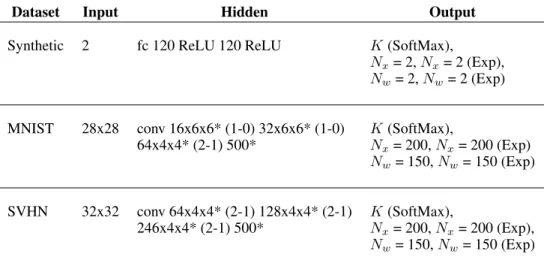
A summary of the results of this and other methods is shown in Table 1. With only a coarse parameter grid search, we achieve classification scores competitive with the current state of the art. Details of the network architecture can be found in Appendix A.

Empirically, we observe that increasing the number of Monte Carlo samples used for gradient prop-agation makes GMVAE more robust to initialisation and in finding all the modes of the data distri-bution. If fewer samples are used GMVAE can occasionally converge faster to poor local minima of the sort of Fig. 2e, missing some of the modes of the data distribution.

(8)

Table 1: Unsupervised classification accuracy for MNIST (reported as percentage of correct labels)

Method K Best Run Average Run

CatGAN (Springenberg, 2015) 20 90.30

-AAE (Makhzani et al., 2015) 16 - 90.45±2.05 AAE (Makhzani et al., 2015) 30 - 95.90±1.13

DEC (Xie et al., 2015) 10 84.30

-GMVAE (M = 1) 10 87.71 74.47±10.20

GMVAE (M = 10) 10 93.67 86.94±6.62

GMVAE (M = 1) 16 88.36 84.80±3.11

GMVAE (M = 10) 16 97.50 90.24±5.74

4.2.1 IMAGEGENERATION

So far we have argued that GMVAE picks up natural clusters in the dataset, and that these clusters share some structure with the actual classes of the images. Now we train GMVAE withK= 10on MNIST to show that the learnt components in the distribution of the latent space actually represent some meaningful property of the data. First, we note that there are two sources of stochasticity in play when sampling from GMVAE, namely

1. Samplingwww from its prior, which will generate the means and variances ofxxxthrough a neural networkβ; and

2. Samplingxxxfrom the GMM determined bywwwandzzz, which will generate the image through a neural networkθ.

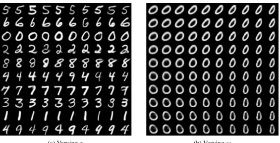
In Fig. 3a we explore the latter option by settingwww = 0and sampling multiple times from the resulting GMM. Each row in Fig. 3a corresponds to samples from a different component of the GMM, and it can be clearly appreciated that samples from the same component consistently result in images from the same digit. This confirms that the learned latent representation contains well differentiated clusters, and exactly one per digit. Additionally, in Fig. 3b we explore the sensitivity of the generated image to the GMM components by smoothly varyingwww and sampling from the same component. We see that whilezzzreliably controls the class of the generated image,wwwsets the “style” of the digit

Finally, we show in Fig. 4 images sampled from a GMVAE trained on SVHN, with and without CV regularisation. Activating CV results in more distincts clusters, spanning wider sections of the space and highlighting more relevant features of the images.

5 CONCLUSION

We have introduced a class of variational autoencoders in which the latent encoding space has the form of a Gaussian mixture model, and specified a generative process that allows us to formulate a variational Bayes optimisation objective. We then discuss the undesirable implications for unsuper-vised clustering of variational mean-field methods, which result in a problematic term involving the prior distribution over cluster labels. Importantly, we alleviate this problem by introducing a prin-cipled regularisation term based on an information-theoretic measure calledconsistency violation. Our experiments show that including this term is necessary for effective deep unsupervised cluster-ing, and in combination with the standard variational Bayes approach can uncover natural cluster structure in the data.

We evaluate our model on unsupervised clustering tasks using popular datasets, achieving competi-tive results compared to the current state of the art. Finally, we show via sampling from the gener-ative model that the learned clusters in the latent representation correspond to meaningful features of the visible data. Images generated from the same cluster in latent space share relevant high-level features (e.g. correspond to the same MNIST digit) while being trained in an entirely unsupervised manner.

(9)

(a) Varyingz (b) Varyingw

Figure 3: Generated MNIST samples: (a) Each row contains 10 randomly generated samples from different Gaussian components of the Gaussian mixture. The GMVAE learns a meaningful generative model where the discrete latent variableszcorrespond directly to the digit values in an unsupervised manner. (b) Samples generated by traversing aroundw space, each position of w

correspond to a specific style of the digit.

(a)α= 0.0 (b)α= 0.4

Figure 4: Generated SVHN samples: Each row corresponds to 10 samples generated randomly from different Gaussian components. GMVAE groups together images that look similar in terms of fonts and colours as opposed to taking into consideration the digit itself, i.e. they are clustering based on visual similarity as opposed to semantic.

Altogether, we have advanced the state of the art in deep unsupervised clustering both in theory and practice, while showcasing the power of information-theoretic considerations in unsupervised learning.

(10)

ACKNOWLEDGMENTS

We acknowledge NVIDIA Corporation for the donation of a GeForce GTX Titan Z used in our experiments. We would like to thank Jason Rolfe for spotting a mistake in the first version of this paper.

REFERENCES

Charu C Aggarwal and Chandan K Reddy. Data clustering: algorithms and applications. CRC Press, 2013.

Christopher M Bishop. Pattern recognition and machine learning. 2006.

Xi Chen, Yan Duan, Rein Houthooft, John Schulman, Ilya Sutskever, and Pieter Abbeel. Info-gan: Interpretable representation learning by information maximizing generative adversarial nets.

arXiv preprint arXiv:1606.03657, 2016.

J. Chung, K. Kastner, L. Dinh, K. Goel, A. Courville, and Y. Bengio. A Recurrent Latent Variable Model for Sequential Data.ArXiv e-prints, June 2015.

Thomas M. Cover and Joy A. Thomas. Elements of Information Theory. Wiley, Hoboken, 2006. ISBN 9780471748816.

SM Eslami, Nicolas Heess, Theophane Weber, Yuval Tassa, Koray Kavukcuoglu, and Geoffrey E Hinton. Attend, infer, repeat: Fast scene understanding with generative models. arXiv preprint arXiv:1603.08575, 2016.

Ian Goodfellow, Jean Pouget-Abadie, Mehdi Mirza, Bing Xu, David Warde-Farley, Sherjil Ozair, Aaron Courville, and Yoshua Bengio. Generative adversarial nets. InAdvances in Neural Infor-mation Processing Systems, pp. 2672–2680, 2014.

Klaus Greff, Antti Rasmus, Mathias Berglund, Tele Hotloo Hao, J¨urgen Schmidhuber, and Harri Valpola. Tagger: Deep unsupervised perceptual grouping. arXiv preprint arXiv:1606.06724, 2016.

Karol Gregor, Ivo Danihelka, Alex Graves, Danilo Rezende, and Daan Wierstra. Draw: A recurrent neural network for image generation. InProceedings of The 32nd International Conference on Machine Learning, pp. 1462–1471, 2015.

I. Higgins, L. Matthey, X. Glorot, A. Pal, B. Uria, C. Blundell, S. Mohamed, and A. Lerchner. Early Visual Concept Learning with Unsupervised Deep Learning. ArXiv e-prints, June 2016.

Matthew J Johnson, David Duvenaud, Alexander B Wiltschko, Sandeep R Datta, and Ryan P Adams. Composing graphical models with neural networks for structured representations and fast infer-ence.arXiv preprint arXiv:1603.06277, 2016.

Diederik Kingma and Jimmy Ba. Adam: A method for stochastic optimization. arXiv preprint arXiv:1412.6980, 2014.

Diederik P Kingma and Max Welling. Auto-encoding variational bayes. arXiv preprint arXiv:1312.6114, 2013.

Diederik P Kingma, Shakir Mohamed, Danilo Jimenez Rezende, and Max Welling. Semi-supervised learning with deep generative models. InAdvances in Neural Information Processing Systems, pp. 3581–3589, 2014.

Yann LeCun, L´eon Bottou, Yoshua Bengio, and Patrick Haffner. Gradient-based learning applied to document recognition. Proceedings of the IEEE, 86(11):2278–2324, 1998.

Alireza Makhzani, Jonathon Shlens, Navdeep Jaitly, and Ian Goodfellow. Adversarial autoencoders.

Yuval Netzer, Tao Wang, Adam Coates, Alessandro Bissacco, Bo Wu, and Andrew Y Ng. Reading digits in natural images with unsupervised feature learning. 2011.

(11)

Danilo Jimenez Rezende, Shakir Mohamed, and Daan Wierstra. Stochastic backpropagation and approximate inference in deep generative models. arXiv preprint arXiv:1401.4082, 2014. C. K. Sønderby, T. Raiko, L. Maaløe, S. K. Sønderby, and O. Winther. Ladder Variational

Autoen-coders.ArXiv e-prints, February 2016.

Jost Tobias Springenberg. Unsupervised and semi-supervised learning with categorical generative adversarial networks. arXiv preprint arXiv:1511.06390, 2015.

Greg Ver Steeg, Aram Galstyan, and Fei Sha. Demystifying information-theoretic clustering. In Pro-ceedings of The 31st International Conference on Machine Learning; arXiv: 1310.4210. Citeseer, 2014.

Martin J Wainwright and Michael I Jordan. Graphical models, exponential families, and variational inference. Foundations and TrendsR in Machine Learning, 1(1-2):1–305, 2008.

Junyuan Xie, Ross Girshick, and Ali Farhadi. Unsupervised deep embedding for clustering analysis.

A

NETWORK

PARAMETERS

For optimisation, we use Adam (Kingma & Ba, 2014) with a learning rate of10−4 _{and standard} hyperparameter valuesβ1 = 0.9,β2 = 0.999and= 10−8. The model architectures used in our experiments are shown in Tables A.1, A.2 and A.3.

Table A.1: Neural network architecture models ofqφ(xxx, www, zzz): The hidden layers are shared betweenq(xxx),q(www)andq(zzz)except the output layer where the neural network is split into 5 output streams, 2 with dimensionNx, 2 with dimensionNw and 1 with dimensionK. We exponentiate the variance components to keep their value positive. An asterisk (*) indicates the use of batch normalization and ReLU layer. For convolutional layers, the numbers in parentheses indicate stride-padding.

Dataset Input Hidden Output

Synthetic 2 fc 120 ReLU 120 ReLU K(SoftMax),

Nx= 2,Nx= 2 (Exp),

Nw= 2,Nw= 2 (Exp)

MNIST 28x28 conv 16x6x6* (1-0) 32x6x6* (1-0) K(SoftMax),

64x4x4* (2-1) 500* Nx= 200,Nx= 200 (Exp)

Nw= 150,Nw= 150 (Exp)

SVHN 32x32 conv 64x4x4* (2-1) 128x4x4* (2-1) K(SoftMax),

246x4x4* (2-1) 500* Nx= 200,Nx= 200 (Exp),

(12)

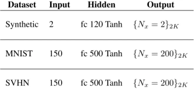
Table A.2:Neural network architecture models ofpβ(xxx|www, zzz): The output layers are split into2K streams of output, whereKstreams return mean values and the otherKstreams output variances of all the clusters.

Dataset Input Hidden Output Synthetic 2 fc 120 Tanh {Nx= 2}2K

MNIST 150 fc 500 Tanh {Nx= 200}2K

SVHN 150 fc 500 Tanh {Nx= 200}2K

Table A.3: Neural network architecture models ofpθ(yyy|xxx): The network outputs are Gaussian parameters for the synthetic dataset and Bernoulli parameters for MNIST and SVHN where we use sigmoid function to keep value of Bernoulli parameters between 0 and 1. An asterisk (*) indicates the use of batch normalization and ReLU layer. For convolutional layer, the numbers in parenthesis indicate stride-padding.

Dataset Input Hidden Output

Synthetic 2 fc 120 ReLU 120 ReLU {2}2

MNIST 200 500* full-conv 64x4x4* (2-1) 32x6x6* (1-0) 28x28 (Sigmoid) 16x6x6* (1-0)

SVHN 200 500* full-conv 246x4x4* (2-1) 128x4x4* (2-1) 32x32 (Sigmoid) 64x4x4* (2-1)