Hedging residual value risk using derivatives
Université Université de Paris Ouest Nanterre La Défense
(bâtiments K et G)
200, Avenue de la République
92001 NANTERRE CEDEX
Tél et Fax : 33.(0)1.40.97.59.07
Document de Travail
Working Paper
2009-31
Sylvain Prado
E
c
o
n
o
m
i
X
http://economix.u-paris10.fr/
Hedging residual value risk using derivatives
Sylvain Prado1
December 2008
Abstract
In the leasing industry the lessor faces a risk, at the end of the contract, in not recovering su¢ cient capital value from resale of the asset. We propose a model to hedge residual value risk using the Gaussian copula methodology. After discussing residual value risk and credit risk modelization, a new derivative product is introduced and analyzed; the Collateralized Residual Values (CRV). The model is applied to an European auto lease portfolio of operating lease contracts pertaining to a major company. Our results indicate that the …nancial product is easy to customize, and to implement through the contract characteristics and the level of correlation.
Keywords: residual value risk, credit risk, credit derivatives, factor modeling, copula.
JEL Classi…cation: C10, G13.
1Senior Asset Analyst at GE Capital Solutions Europe in London, UK.
PhD Candidate at the University of Paris. Member of ‘EconomiX’ group in Paris, France. T +44 (0) 20 8754 2256
F +44 (0) 20 8754 2288
E [email protected] [email protected] Meridian Trinity Square
23-59 Staines Road Hounslow, Middlesex TW3 3HF, UK
1
Introduction
A lease is a contract in which one party transfers the use of an asset to another party for a speci…c period of time, at a predetermined rate. Leasing equipment is an important means of …nancing, and consequently represents a signi…cant part in many …nancial institutional portfolio. In 2006, leasing represented more than one-sixth of the world’s annual equipment …nancing requirement 2. The value of the entire Global
leasing market was estimated to be more than $633 billion3. Academic results suggest that “leasing allows
small …rms to …nance their growth, and/or survival while for large …rms, leasing appears to be a …nancial instrument used by sophisticated …nancial managers to minimize the after-tax cost of their capital“4.
In the leasing industry, residual values are the forecasted prices of equipment in the second hand market. A large part of the rent paid by the customer during a life contract is the di¤erence between the list price and the residual value. The leasing company makes money or losses money depending on whether it accurately predicts the value of the asset at the end of the contract (fair market value). If residual values are forecasted to be higher than what the asset is actually worth at lease-end, then there will be a loss. At the opposite, if residual values are forecasted to be lower, then there will be a gain on resale.
In the European auto lease market, most leases are closed-end leases: leasing companies assume the residual value risk. In 2001, car resale’s price fell dramatically, as a result; US leasing companies su¤ered large losses, and some even dropped out of the business5. Residual value risk is a key element in the leasing
industry, however; there is minimal literature, and few developed models. The few studies were developed in three main areas; Operational Purpose6; The operational perspective aims to set the most accurate residual
2Percentage market penetrations are highly signi…catives in United states (27.7%), Germany (23.6%), and Spain (29.1%). 3According to the White Clarke Global Leasing report (2008), "Globally, the industry contnued to growth robustly, with the
top 50 countries increasing volume by 8.8%" between 2005-2006. The Percentage of the world market volume was respectively 41.1% and 38% for Europe and North America.
4See Lasfer and Levis (1998)
5See Gordon (2001) for a description of the 2001 Leasing industry crisis.
6Jost and Franke (2005) illustrate the use of a speci…c tool of statistical modelling to calculate residual value through a wide
range of parameters. In Lucko (2003) and Lucko, Anderson-cook, and Vorster (2006), residual values are set using regression methodology. Rode, Paul, and Dean (2002) outline a framework for analysing the uncertainty of residual value for assets, such as power generation facilities, for which few data points exists.
value; Basel 2 requirements7; de…nes how to calculate reserves. Studies evaluate Basel 2 accuracy, and reserve
calculation in relation to speci…c credit risk in the leasing industry, and Leasing Contract Valuation8; in the
valuation analysis, the residual value risk is included through an American option. It allows a comparison of leasing (…nancial lease and operating lease) v.s. purchase decision. Unfortunately, it does not aim to hedge the speci…c Residual value risk, let-alone the correlation issue in a portfolio of equipment.
A lack of development on …nancial products hedging residual value risk, sent my research to credit risk. The recent important developments in …nance modelling and in new …nancial products were in credit derivatives. This implies a change in credit management involving banks and other …nancial institutions. A credit derivative is a contract between two parties that allows the use of a derivative instrument to transfer credit risk from one party to another. The risk seller, in form, has to pay a fee to the risk buyer who will take the risk. Over the last ten years, the credit derivative market has faced a substantial increase. A lot of credit risk models have been developed, therefore; increasing investor interest9.
In 1999, Li‘s Gaussian copula model10facilitated a dramatic success of this derivative sector. He proposed
a fairly easy, and intuitive model depicting the payment default of a company like the survival probability of a human life11. It was also a new tool to evaluate the ongoing issue of credit risk; i.e. correlation. For
instance, in a basket of loans there is an individual risk component. Each loan has a risk to default its payment. The systemic risk is the other component. An economic downturn could also impact the whole portfolio, and the systemic risk implies correlation.
Collateralized Debt Obligation (CDO) turns the correlation problem into a solution. It is a credit
7Schmit produced several articles on Credit risk in leasing industry to analyse Basel 2 requirements accuracy. See Schmit
(2003), Schmit (2004), Irotte, Schmit, and Vaessen (2004), Laurent and Schmit (2007).
8T. Copeland and J. Weston (1982) apply an American put with a decreasing exercise price and S.E Miller (1995) includes
an American Call Option in a net present value formula to estimate the internal rate of return of the deal. S.R Grenadier (1995), focusing on the real estate arena, adds a residual value insurance that is equivalent to a put option on the underlying asset in the pricing of a varriety of leasing contracts.
9“At the risky end of …nance” The economist (April 21st 2007) gives an up to date on the credit derivatives market:
“According to the Bank for International Settlements, the nominal amount of credit-default swaps had reached $20 trillion by June last year. With volumes almost doubling every year since 2000, some reckon the CDS market will soon be worth more than $30 trillion”.
1 0See Li (2000).
derivative created from a portfolio of debt instruments12. The risk seller transfers the risk, therefore; the
risk buyer takes the risk. Of course, the risk seller has to pay a fee to the risk buyer. The CDO became a successful product by allowing the credit risk division among di¤erent tranches. Synthetic CDOs13, in particular, were booming, improving liquidity, and allowing corporate bonds to be sliced and diced on the basis of risk. Investors were able to choose di¤erent levels of risk and returns14. The growth was so huge
that it had a global macroeconomic impact, decreasing the risk of default impact, in‡ating asset prices and narrowing credit spreads15. Prior to summer 2007, there was up to 30% of banking investment pro…t.
From that time, all products have slumped suddenly in value due to fraud, and low quality loan underwrit-ing. The "credit crunch" allowed identi…cation of several weaknesses in the industry of loan securitization. Severing the link between borrowers and risk takers, it promoted a lack of accountability. In addition, market protagonists contributed to a credit bubble16. Investor did not fully understand the products and had an over reliance on ratings provided by specialized agencies. Moreover, some securities were poorly structured. Thereby, on a cleared market with more incentives, some experts are hoping for a recovery. Fortunately, securitization is not con…ned to consumer or corporate loans.
Residual value risk and credit risk have a clear analogy, constituting of units that are more or less risky. A lease portfolio is similar to a loan portfolio, both could be divided into systematic and idiosyncratic risks. Losses occur when certain events happen, and again, the correlation risk has a huge impact. Hedging a portfolio of leasing equipment using derivative securities is attractive, and the idea to use some of the signi…cant developments in Credit risk modelling is attractive as well.
1 2“Collateralized debt obligations divide the credit risk among di¤erent tranches: First senior tranches (rated AAA), second
mezzanine tranches (AA to BB), and …nally equity tranches (unrated). Losses are applied in reverse order of seniority. Therefore junior tranches o¤er higher coupons to compensate for the added risk”.
1 3“Synthetic CDOs do not own cash assets like bonds or loans. Using credit default swaps (a derivatives instrument), synthetic
CDOs gain credit exposure to a portfolio of …xed income assets without owning those assets”.
1 4See Hull (2005)
1 5« La multiplication des émissions de CDO semble avoir contribué au resserrement prononcé de spreads intervenu au cours
de ces eux dernières années sur l’ensemble des marché de crédit » . Cousseran and Rahmouni (2006).
« This derivatives “money” is not being used to buy food, clothes or cars, which is why there has been no general pick-up in in‡ation. But it has been used to in‡ate asset prices, Mr Roche [Independent Strategy] argues » . “At the risky end of …nance” The economist (April 21st 2007).
Therefore the aim of this research is to transfer a model from the Credit risk to the Residual risk. The one factor model is presented and modi…ed. This modi…cation allows the creation of a new product, the Collateralized Residual Value. Pykhtin and Dev (2003), …rst applied the one factor model to auto lease. They calculated the economic loss associated to Residual risk, leading to an estimate on economic capital. The model was constructed and modi…ed for …nancial lease with the option to buy out (the lessee has a purchase option at the end of the contract). Moreover, loss distribution was calculated for a …ne grained portfolio (speci…c to large portfolio without signi…cant individual exposure), as a result, the model was only driven by the systematic factor.
Our study di¤ers slightly, as we aim to hedge residual risk using a derivative …nancial product. This article is intended for people within the leasing industry interested by an innovative …nancial product, as well as people from the …nancial market concerned by leasing risk opportunities. More speci…cally, we aim to hedge risk for a classical European contract. The product should cover operating lease contracts on a de…ned number of units and de…ned characteristics equipment parameters. We complete this theoretical development by an empirical analysis in which we confront this new derivative with market reality. Research gathered is organized as follow: Sections 2 and 3 provide some backgrounds on residual value risk and CDO pricing; Section 4 describes the model and the …nancial product; Section 5 is an empirical analysis and Section 6 concludes.
2
Leasing
The initial idea of leasing is that it is the use of equipment in a business which produces bene…ts, not the ownership. One characteristic of ownership in leasing contract is residual value risk that generates competitiveness or losses.
2.1
Main characteristics
As previously mentioned, a lease17 is a contract between two parties where a party (the lessor) provides
equipment for usage on a speci…c period of time to another party (the lessee) for speci…ed payment. Three parties are involved in the process; equipment suppliers, lessors and lessees. The lessor is the party that grants the use of the asset to the lessee. The lessee is the party that obtains the use of the asset from the lessor. The lessor purchases the equipment to the supplier. All along the contract, the lessor has the legal ownership of the asset. To use the asset the lessee makes periodic payments to the lessor at an agreed rate of interest.
There are two families of lease contracts. An operating lease can be considered as a typical rental allowing the lessee to use an asset without owning it. A…nancial leaseaims to transfer all risks and rewards of ownership to the lessee.
A lease is de…ned as a …nancial lease if it contains one of the following elements:
The ownership of the asset is transferred to the lessee by the end of the lease term.
The lessee has an end of contract option to buy the asset lower than the fair market value.
1 7Leasing de…nitions and legislations are quite di¤erent from a country to another. As we do not wish to focus on a speci…c
Whether the asset is transferred or not, the lease period is for a majority of the asset useful life.
Because of the specialized nature of the asset, the lessee only can use the equipment without major modi…cation.
Otherwise, it is an operating lease18.
A lease is a …nancial instrument for the procurement of equipment. Recovery rate on a lease is higher than on a standard loan. But why do enterprises lease ? Regarding large …rms, leasing minimizes the after tax cost of their capital. For small asset base companies, leasing increases access to equipment …nance. The inherent value of the purchased asset acts as collateral. The lessor is the owner of the equipment, and then is secured by the collateral. Another attractiveness is the leasing companies expertise. Leasing companies are not only intermediaries. Their expertise is a real value added in the leasing process. They have knowledge of the asset. They select the appropriate equipment based on the ability of the asset to contribute to cash ‡ow (through various parameters like equipment characteristics, economic life of the asset, taxes or residual value risk). Leasing companies have also skills in …nance, credit, equipment acquisition and dealing. All things considered, they facilitate the ‡ow between equipment suppliers and equipment users.
On lessor side, they are several key elements:
Asset leased: Used by the lessee for business purpose, it could be any kind of equipment (i.e. printers, trucks...)
Asset List price: The lessor is usually able to negotiate rebates and the lessee could be part of the acquisition process.
Lease period: It is a pre requisite agreement between the parties. According to the contract, it could be ‡exible .
End of term options: At the end of the contract, they are options allowed to the lessee; Lease period can be extended, lease can be renewed, equipment can be bought or returned.
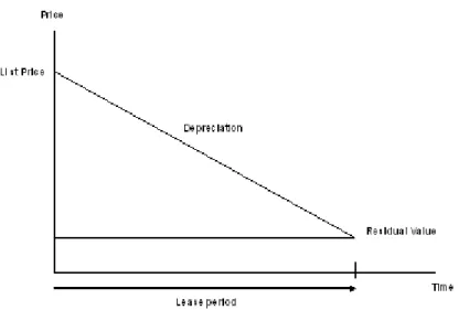
Residual value: The lessor forecasts the market value of the asset at the end of the contract.
Depreciation: It might be seen as the variance between the List price and the Residual value all along the lease period.
Lease payment: As illustrated by Figure 1, several features are included in payments made by the lessee during the contract; depreciation of the asset (usually the larger component), interests on the lessor investment, servicing charges (including operation cost, insurances, counselling, repairs...).
2.2
Residual value risk versus competitiveness
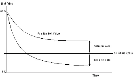
The residual value risk is that the lessor faces the risk to not being able to recover su¢ cient capital value from the resale or disposal of the asset. As illustrated by Figure 2, the fair market value curve implies a gain on sale or a loss on sale depending on the level of residual value.
Figure 2: Depreciation curve
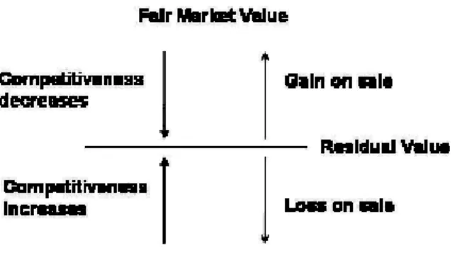
Therefore the lessor has a dilemma: The higher the residual value, the lesser the risk of loss on sale. But the higher the residual value, the lower the rental payment. At the same time, the lower the rental payment, the better the competitiveness. And conversely the less the residual value risk, the worse the competitiveness. Figure 3 displays the mechanism of competitiveness and sales results at the end of the contract.
Figure 3: Dynamical bene…ts
In others words, the lessor has to set a residual value to minimizing residual value risk and maximizing competitiveness. A solution would be the use of a …nancial product. Hedging residual value risk could be done through a security derivative. Security de…nition includes …nancial security (bond, stock) but also capital market securities (mortgage, long-term bonds). It is an investment instrument which o¤ers evidence of debt or equity. A security derivative is a …nancial security whose value is derived in part from the value and characteristics of another security, the underlying asset19. It would allow the lessor to transfer the risk
to a fourth party (i.e. insurance company, …nancial market...).
3
Model pre requisites
Because it allows to create a link of two survival functions, Gaussian Copula is a key element in our analysis. CDO pricing, default modeling, and the one factor model are also inherent to the …nancial product presented in Section 4.
3.1
CDO are a subclass of ABS
Asset Backed Securities are securities backed by a pool of assets. ABS include various subclasses ( Commer-cial Mortgage Backed Securities (CMBS) or credit card ABS...), depending on the underlying asset class. Obligations are usually underlying Collateral Debt Obligation (CDO). The basic idea of CDO is to pool corporate bonds and selling o¤ pieces of the pool. A synthetic CDO replaces pool’s bonds by speci…c credit derivatives, Credit Default Swaps (CDS).
All in all, CDS are triggered by a credit event. A credit event increases the likelihood that the rating of a bond decreases. Consequently, a credit event increases the risk that a bond issuer will default, by failing to repay principal and interest in a timely manner. The events triggering a credit derivative are de…ned in a bilateral swap con…rmation. It is a document that refers to an agreement between the two swap counterparts. There are several standard credit events that could be referred to in credit derivative transactions: Bankruptcy, Failure to Pay, Restructuring, Repudiation, Moratorium.
By selling a CDS, an investor can take exposure to an individual credit. He is receiving periodic payment from his client. At the same time, however, he has to pay contigent payment when default occurs. The client, conversely, can hedge individual credit by buying a CDS. He provides periodic payment to the client and receives contingent when default occurs.
3.2
Default, default, default....
Default modeling is about the expected default payment of an obligor in a bank credit portfolio. The obligor (or debtor) is an individual or company that owes debt to another individual or company (the creditor). The obligor borrows or issues bonds.
The following framework de…nes our model. The model is underlaid by a probability space. This proba-bility space is constituted of three parts. F, a Algebra, is the information available into a sample space called . Elements of F are the measurable events of the model. Events of default are measurable. For instance, the event that an obligor survives or defaults is a measurable event. The last element is Pr, a probability measure. Pr(default)is the probability of default. Finally, to summarize, the probability space
( ;F;Pr)is underlying our model.
In survival analysis,T is a random variable denoting the time of default andt are others di¤erent times. IfT > t, then the obligor defaults. The survival function, usually denotedS is de…ned asS(t) = Pr(T > t). This function must be non increasing: S(t+ 1) S(t).
We can now de…ne the complement of the survival function. Usually denotedF, it is alifetime distribution function: F(t) = P r(T t) = 1 S(t). From this concept a default rate per unit time can be calculated, theevent density. Usually denotedf, it is the derivativef(t) =dtdF(t).
All of this allows the creation of an advanced function, thehazard function. The hazard function,usually denoted , is the event rate at time t conditional until time t or later. It is given by (t)dt = Pr(t T < t+dt j T > t) = fS(t()tdt) = SS0((tt))dt ( (t) 0 and R01 (t)dt =1 with no continuous or monotonic constraints).
A cumulative hazard function is (t) =R0t (u)du.
Because (t) = SS0((tt)), then dtd (t) = SS0((tt)) and (t) = logS(t).
Several distributions can be used in duration modeling (usually de…ne on R+), the most common one being the exponential distribution (S(t) =et).
3.3
Basic elements on Copulas
Why do we use copula ? In a portfolio, credit risks are non independent. Copulas are a convenient approach to specify a joint distribution of survival times. Using a copula function, we are able to link the survival function of an obligor to the survival function of another obligor in a portfolio .
In our model, we use copula on a three dimensional perspective. For simpli…cation purpose, we will focus on thebivariate distribution function and the two dimensional copula. The following results, however, can be extended to the multivariate case (see Nelsen (2006) and Vershuere (2006)).
For a "rigorous" copula de…nition, we …rst have to de…ne theunit square and the concept ofsubcopula.
The unit square I2 is the productI IwhereI= [0;1].
A two dimensional subcopula is a functionC0 de…ned through the four following properties: 1_DomC0=S1 S2(withS1andS2 are subsets ofIcontaining0and1).
2_C0is grounded20.
3_C0is 2-increasing (for every x1 x2 andy1 y2 ,H(x1; y1) H(x2; y2)). 4_ For every uin S1 and everyv inS2,C0(u;1) =uandC0(1; v) =v.
We are now able to de…ne atwo dimensional copula: It is a two dimensional subcopulaC whose domain isI2.
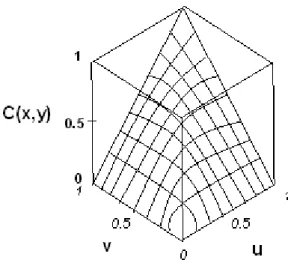
Figure 4 gives an intuitive notion of a two dimensional copula. The graph of a two dimensional copula is a continuous surface within the unit cubeI3.
2 0A function H fromS1 S2is grounded ifH(x; a2) = 0 =H(a1; y)for all(x; y)inS1 S2 witha1 anda2last elements of
Figure 4: Two dimensional copula
Two others elements are fundamental in our analysis; the joint bivariate distribution function and the Sklar Theorem.
A joint bivariate distribution functionis a functionH with domainR2 such thatH is 2-increasing:
H(x; 1) = H( 1; y) = 0, and H(+1;+1) = 1. The joint bivariate distribution function is a key element of the Sklar Theorem: Let H be a joint distribution function with margins F and G. Then there exists a copula C, such that for allx; yin R,H(x; y) =C(F(x); G(y)): Furthermore, ifF andG are continuous, the copulaC is unique. OtherwiseC is uniquely determined on RanF RanG. Conversely, if
C is a copula andF andGare distribution functions, then H is a joint distribution function with margins
F andG:
We can now include random variables. LetX andY be random variables with distributions functionsF
andG, and joint distribution functionH. Then there exist a copulaC withH(x; y) =C(F(x); G(y)). IfF
In a few words, a copula function is a function that links univariate marginal to their full multivariate distribution:C(u; v) = Pr(u U; v V). Therefore, using a copula function, we are able to link the survival function of a credit risk to the survival function of another credit risk in a portfolio.
3.4
Speci…c pre requisites, the Gaussian copula
In the model presented in this article, we use the Gaussian copula. Let be the bivariate normal distribution
function with correlation coe¢ cient (0 1). The bivariate normal is a member of the family of
elliptically contoured distributions. The density function of is (x; y) = 1
2 p1 2e
( 1
2(1 2 )(x2+y2 2 xy)).
The densities for such distributions have contours that are concentric ellipses with constant eccentricity.
1 is the inverse of a normal distribution function.
Finally the Gaussian copula is C(u; v) = 2( 1(u); 1(v); ).
Consequently variables are jointly elliptically distributed and we can set using a linear correlation as a measure of dependence: LetX andY follow, respectively, the distributionF andG. They jointly follow the distribution functionH. Then the linear correlation forX andY is de…ned, usingu=F(x)andv=G(y)
as = (X; Y) = p 1 V ar(X)pV ar(Y) R1 0 R1 0[C(u; v) uv]dF 1(u)dG 1(v).
Another property of the bivariate normal distribution is radially symmetry. A bivariate normal distrib-ution with parameters x, y, 2
x, 2y and is radially symmetric about the point ( x, y). It means that
H( x+x; y+y) =H( x x; y y).
Using copula, we are able to work on survival function. Indeed, for a pair of random variable with joint distribution function H(H(x; y) = P[X < x; Y < y]), the joint survival function copula is given by
H(x; y) = P[X > x; Y > y] = 1 H(x; y). The relationship is H(x; y) = 1 F(x) G(y) +H(x; y) = 1 +F(x) +G(y) +C(1 F(x);1 G(y)).
In the next section, we assume that the correlation of default is driven by a common factor through a Gaussian copula.
3.5
The initial one factor model is used for CDO pricing
To resume the model in one sentence, a …rm defaults when its “asset value-like” stochastic processX, falls below a barrier. X is commonly identi…ed as the amount of asset and X the barrier as the amount of liabilities. The …rm defaults when the amount of asset is below the amount of liabilities. The idea was …rst introduced by Merton (1974). He transferred an option pricing model to the credit risk market. Then he applied the Black and Scholes model to credit risk. We present an alternative model using copula. Value added is in copula ‡exibility to dependent variables and copula ability to provide scale invariant measure of association between random variables. The intuitive aspect of this model contributed to the growth of credit risk market.
The model described below is the famous standard Gaussian copula developed by Li (2000) and exposed21
by Gibson(2004).
In a reference portfolio of i= 1; :::N credits, for each obligor, default payment occurs whenxi (reference credit normalized asset value) falls belowxi (the threshold).
xi=aiM+
q
(1 a2
i)Zi (1)
xi has three main components: M,Zi, andai.
M is the common factors a¤ecting all the credits, the systematic risk. Zi is the factor a¤ecting only crediti. ai is the correlation parameter(06ai 61)and de…nes default dependency between companies in the economy. The correlation of asset value between creditsi andj is equal toaiaj. The random variables are assumed to be independently distributed. Therefore unconditionally on the systematic risk, default payments are correlated but conditionally there are independent.
M,Zi, andxiare means-zero, unit variance random variables with distribution functionsG(0; 1),Hi(0; 1),
2 1See also Meneguzzo and Vecchiato (2004) for an empirical study of credit derivatives within the copula framework.
and Fi(0; 1). qi(t) is a risk neutral probability that credit i default before t. The default threshold xi is equal toF-1
i (qi(t)).
When does a default happen ?
A default happens whenxi falls belowxi.
Butxi falls belowxi ifF(xi)< qi(t),xi< Fi-1(qi(t)),aiM +
p 1 a2 iZi< F 1(qi(t)) and …nally Zi< F 1(q i(t)) aiM p 1 a2 i
Conditional on the value of the factorM, the probability of default is therefore
qi(t=M) =H 1( F 1(q i(t)) aiM p 1 a2 i ) (2)
For any number of default in a portfolio of N obligors, we have to estimate the probability of default on timetand conditional on the common factor M.
Therefore, we set the number of default distribution using a binomial function22.
P N(l;t=M) = l
N qi(t=M) (3)
Once we have the conditional default distribution, we estimate the distribution according the distribution ofM.
The unconditional default distribution PN(l;t)can be calculated as
PN(l;t) =
Z 1 1
PN(l;t=M)g(M)dM: (4)
In a CDO, the investor is responsible for the interval of loss[L; H]. The expected loss of a CDO is de…ned on[L; H]. We de…ne the loss for any default asA(1 R)withA the notional amount of credit andR the
2 2The number of default distribution is usually computed through a recursion method (Andersen, Sidenius and Basu (2003)
recovery rate.
The expected loss is
ELi= N
X
l=0
PN(l;Ti) max(min(lA (1 R); H) L;0) (5)
withT i, i= 1; :::; nthe periodic payment.
Now, how to price a CDO ?
A CDO contract speci…es two potential cash ‡ow streams: a Contingent leg and Fee leg.
On the contingent leg side, the protection seller makes one payment only if the references credit default. The amount of a contigent payment is the notional amount multiplied by (1 R).
The contigent leg is
contigent=
n
X
i=1
Di(ELi ELi 1) (6)
with Di the risk free discount factor for payment datei (e rt, withr the risk free rate). The risk free discount factor is usually derived from the risk free interest rate.
On the …xed leg side, the buyer of protection makes a series of …xed, periodic payments of CDO premium until the maturity, or until the reference credit defaults.
The expected present value of the Fee leg is
F ee=s
n
X
i=1
Di i[(H L) ELi)] (7)
i is the accrual factor for payment date i andsis the spread per annum paid to the tranche investor ( i Ti Ti 1).
The value of the CDO contract to the tranche investor at any given point of time is the di¤erence between the present value of the contigent leg and the present value of the …xed leg. It is the di¤erence between the protection the buyer expects to pay, and the amount he expects to receive.
The Mark To Market value of the tranche, from the perspective of the tranche investor is
M T M =F ee Contigent (8)
At inception the mark to market is equal to 0, therefore the spread is
s= n Contigent
P
i=1
Di i[(H L) ELi)]
(9)
4
A modi…ed model: The leasing model
From equipment leasing speci…cities and the one factor model, we create a residual value risk model. A new product called Collateralized Residual Value (CRV) is adjusted through the leasing contract parameters.
4.1
There is a similarity between credit risk and residual value risk. But there
are also dissimilarities and speci…cally in Auto Lease.
The main idea of the leasing model is that a portfolio of leased equipment is comparable to a portfolio of credit. A portfolio with losses on resales is equivalent to a portfolio of credit with companies defaulting.
As in a CDO, every unit into the lease portfolio, has an idiosyncratic and a systematic risks; asset speci…c characteristic impact is resale price (model type, obsolescence. . . ). At the same time, resale price of other assets has a signi…cant impact (bid and ask e¤ect, downturn on the resale price market,
There are also dissimilarities:
First of all, equipment units are resold only one time at the end of the contract, although for a CDO, there is a risk of default throughout the contract. Therefore, the model presented in next section is set for only one period.
Another dissimilarity (and not the least) is on correlation estimation. Di¤erence is not on calculation but on data source.
In credit risk, they are four main data sources available:
-Default events that are obviously concrete realization of credit risk. They are rare events and as a result there are usually few data available. Approximations and aggregation have to be made to constitute data bases.
-Companies credit ratings: They are provided by credit agencies and re‡ect the credit risk of a company according to experts points of views. By and large, they are made through balance sheet and macroeconomic analysis.
-Credit spreads: They re‡ect market perception of credit risk. A large amount of data is available. But spreads could be impacted by external elements like liquidity
-Equity correlation: The factor model (cf Section 3), assumes a theoretical link between equity and credit risk. Correlations are then more easy to compute.
In residual risk, there is one main data source available: for a residual value calculation, inputs are observations from second hand markets. Correlation estimation of residual value is based on resale market statistics. Resale prices, asset characteristics and price index are used to set modelization variables. A large amount of data is available.
The last dissimilarity is on standard de…nitions. As multiple factors de…ne a resale, there are issues to de…ne resale asset classes or homogeneity prices.
Auto lease is an extreme illustration. The high price level in the automotive second hand market involves a high residual value level. Combined to a competitive leasing market, the level of price leads to high risks of loss on sale.
At the same time, automotive is a singular equipment. A car is not only a tool to go from a place to another. It is also a living place and a symbol. Automotive often re‡ects driver’s sociological characteristics. The purchase of a vehicle is a sensitive act, even in business. Therefore, Auto lease is a wide area to analyze. In automotive market multiple factors in‡uence resale price. A second hand vehicle price is impacted by age (time between registration date and resale date), mileage (number of kilometers at the end of the contract), damages (i.e. amount and type ), product life cycle (i.e. new model...), make (i.e. Toyota, Renault...), model (i.e. Yaris, Laguna...), version, body type (i.e. break, pick-up...), segment (i.e. small cars...) or external color. Figure 5 gives an overview. Choices have to be made to de…ne similar assets and prices (c.f Section 5).
4.2
Homogeneous equipment type model
The initial idea is simple: we use the equipment resale value as the asset value-likexiand the probability of resale value below residual value (xi<xi) as the probability of default.
In a reference portfolio ofi= 1; :::N units (vehicles, equipment...), for each obligor, losses occur whenxi (reference unit normalized asset value) falls belowxi (reference unit normalized residual value).
xi=aiM+
q
(1 a2
i)Zi (10)
-The correlation of resale’s prices between unitiandj is equal toaiaj.
-M is the sectorial factor a¤ecting equipment units on resale’s market andZi is the risk of loss on resales on uniti
-Xi, M, and Zi are means-zero, unit variance random variables with distribution functions Fi(0; 1),
G(0; 1), andHi(0; 1).The random variables are assumed to be independently distributed.
At that point, the construction is similar to the credit model, but we include residual risk. Resale’s value can be lower than residual value. There is a risk of loss on sale.
Three new elements will have an impact on the leasing adjustment of the model.
Viis the residual value or in other words the expected fair market value. mF M Viis the historical average fair market value,eF M Vi is the historical standard deviation.
mF M Vi, eF M Vi, and Vi are set on a percentage of Lp, List price by unit. As an example, an asset boughte10000 and leased for a Residual value of e5000 hasVi= 50%.
Then residual risk is added: Probability of loss at the end of the contract is qi(t). qi(t) is a variable with meanmF M Vi, varianceeF M Vi, and distribution functionEi(mF M Vi;eF M Vi)The probability of loss depends on residual value: qi=Ei(Vi). So default thresholdxi is equal toFi-1(qi).
Conditional on the value of the sectorial factorM, the probability of default is therefore qi(M) =H 1( F 1(qi) aiM p 1 a2 i ) (11)
Again, conditional probability isPN(l;M) = l
N qi(M)and the unconditional probability can be calcu-lated asPN(l) =R1
1P
N(l)g(M)dM.
As a result the recovery rate is equal to the probability of loss. By construction the recovery rate is
R=qi. The loss on sale for any unit is(1 R)Lp. Finally, resale price becomesRLp.
Previous elements allow the creation of a …nancial product, inspired by Collateral debts obligations:
The Expected loss is
EL=
N
X
l=0
P N(l) max(min(Lpl (1 R); H) L;0) (12)
The contigent leg is
contigent=
n
X
i=1
Di(EL) (13)
The premium leg is
F ee=s n X i=1 Di i[(H L) ELi)] (7) The spread is s= n Contigent P i=1 Di i[(H L) ELi)] (9)
4.3
Heterogeneous equipment type model:
a portfolio of three di¤erent assetsThe model is extended to a portfolio with non similar units. A company ‡eet is commonly constituted of various car model. In an European leasing contract for medium size European company, lessee usually request di¤erent categories of cars for an auto lease contract. The ‡eet is usually divided into three groups: Executives’cars (usually high brand car), Employee cars (medium level cars) and Small cars.
Basically the construction is similar to the homogeneous equipment type model (cf Section 4.2). Three representative’s vehicles constitute the model: Ex, Em and Sm.
Now there are di¤erent types of asset residual values, number of units, List price etc....
V1i,V2i,V3i are residual values for group 1, 2, 3
mF M V1i,mF M V2i, mF M V3i, are fair market values historical averages,
eF M V1i,eF M V2i,eF M V3iare historical standard deviation historical averages.
mF M V1i, eF M V1i, andV1i are set on a percentage of List price. The recovery rate for group 1 is
R1 =q1i, the loss on sale for any unit isR1(1 Lp1)withLp1unit list price. Indeed, resale price isR1Lp1. The principle is the same for others groups.
For each vehicle, asset value is stillxi=aiM+
p
(1 a2
i)Zi:
For group 1, default thresholdxiis equal toFi-1(qi)withq1i=Ei(V1i)andEi(mF M V1i;eF M V1i):The principle is the same for other groups.
The distribution of the number of default, conditional on the common factor M, is computed for each group asPN1(u;M) = u N1 q1i(M),P N2(v;M) = v N2 q2i(M), P N3(w;M) = w N3 q3i(M)withN1; N2; N3
number of units,PN1; PN2; PN3 the conditional probabilities, andu; v; w number of defaults for group 1, 2,
3.
The probability of default is computed on the whole portfolio.
PN(u;v;w;M) =PN1(u;M)PN2(v;M)PN3(w;M)
EL=
N
X
l=0
PN(u;v;w;M) max(min((Lp1u (1 R1))+(Lp2u (1 R2))+(Lp3u (1 R3)); H) L;0) (14)
Premium leg, contigent leg and spread are calculated like in 4.2.
It is straightforward to generalize this approach to more than three vehicle type.
4.4
Collateralized Residual Values
We propose a …nancial product, the Collateralized Residual Values, that covers residual value risk. We display a sensitivity analysis of the CRV to the main characteristics of the leased asset.
4.4.1 A CRV is
a new class of ABS
The Collateralized Residual Values (CRV) is a new class of Asset Backed Securities (ABS). The CRV is inspired by synthetic Collateralized Debt Obligations (CDO) structure. Like a CDO, CRV can be sliced and diced, and tranches can be sold. But CRV is not about credit risk. The purpose is to hedge residual value risk on a portfolio of leases. A credit derivatives, obviously, is more accurate to hedge credit risk in a portfolio of contract.
4.4.2 Sensitivity Analysis on a CRV
What is the sensitivity of a CRV to size, residual value, and fair market variance ?
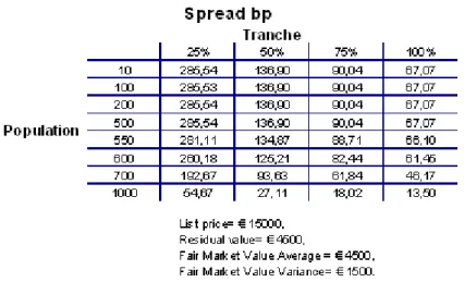
In the following sensibility analysis, all underlying reference assets are cars. The portfolio is homogeneous. List price (e15000), Fair market value (e 4500) and Correlation (p0:3) by car are equal. Cars are leased on a three years contract.
Impact of Fleet Size Table 1 shows that the buyer of protection on a ‡eet of 600 units should be willing to pay 125,21 basis points to hedge the …rst 50% losses using a CRV.
Table 1: Sensitivity to ‡eet size
According to results, the spread is stable until 500 units. Then the increasing size reduces the cost of protection. An increase in size reduces idiosyncratic e¤ect. There is a diversi…cation of risk .
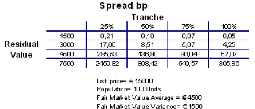
Impact of Residual Value level
Table 2: Sensitivity to residual value
The higher the residual value, the higher the pricing of CRV (Table 2). As illustrated in Section 2.2, decreasing residual value reduces the risk of loss on sales.
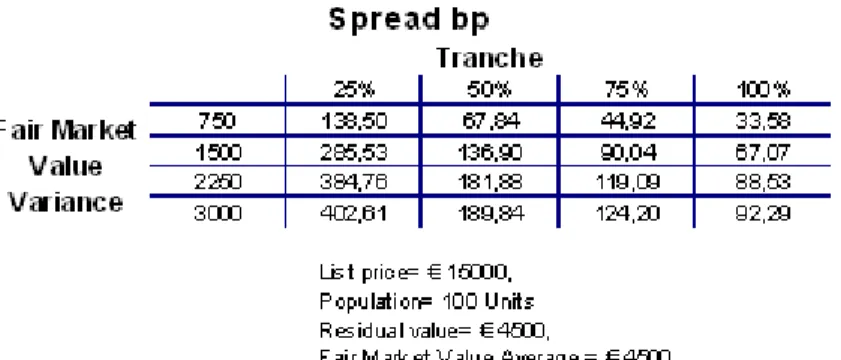
Impact of Fair Market Value variance
Table 3: Sensitivity to fair market value variance
Fair market value distribution tails depends of FMV variance (Table 3). For an higher variance, tail are larger. As a result, the spread is an increasing function of the variance.
5
Empirical Analysis
The model is applied to a six years historic resale’s portfolio. The observations, between 2000 and 2008, are from a major European leasing company (General Electric Capital Solutions). We …rst estimate the correlation of assets to a common factor. Then fair market value parameters and residual value are estimated
5.1
Correlation to the one sector factor
According to section 4.2, we have to set the linear correlation (ai) between the portfolio and a sectorial factor a¤ecting equipment units on resale’s market (M). The sectorial factor is assessed using Eurostat Harmonized Consumer Price index (HCPI23). The index Purchase of vehicles price allows comparison within European
markets. Additionally, a portfolio index has to be created. The portfolio index provides a non-biased historical trend analysis and exposes portfolio sale price at di¤erent time.
5.1.1 Automotive Price Index
To set a common factor that would a¤ect the whole portfolio, several HCPIs are available ; HCPI all items, HCPI Energy, HCPI Petroleum products, HCPI Road transport equipment.
The Index "Purchase of vehicle" (Figure 6) appears to be the most relevant. It covers purchases of new vehicles and purchases of second-hand vehicles from other institutional sectors. It is available by country and on European level. This index is included in the modelization as the sectorial factor indicator (M). Vehicle customers have to choose between resale market and new market. As a consequence, resale market is strongly impacted by new vehicle market. Therefore, a positive or a negative correlation of the sectorial index with the portfolio can be expected.
Figure 6: European HCPI
5.1.2 Portfolio Index Creation and Computation
A large amount of parameters impacts resale price and there is a non homogeneity of the portfolio mix from one month to another. As a consequence, average price never re‡ects accurately portfolio sales price variance through time. Therefore a consistent price variable is created through an index replicating a same arti…cial portfolio. The idea is to replicate a portfolio mix to allow time series analysis.
Portfolio Index Creation The information comes from resale vehicles statistics from 01/2000 to 01/2008 including France, Germany, Italy, Portugal, Spain and Sweden. We only include normal terminations sales (sales types like wrecks or litigations are excluded). Observations with extreme and incorrect values are cleaned. High damages (95th decile by country) that would alter resale’s price and therefore are …ltered.
Calculation is a …ve-steps process:
1 Creation of buckets for Age and Mileage (details in appendix).
age=mileage=model=f iscalclass=f ueltype=country
3. Keys with population of less than 100 units on the whole history are excluded
e.g.:GBR=T oyota=previa=private=lightgoods=petrol=_6:33;39month=_3:75000;105000km is excluded. During the last 8 years, less than 100 units in this bucket have been sold.
Representative and similar samples are created all along the history using the historical key frequency:
4. A Random selection is processed by month through the following criteria: 1% of units by bucket are selected:
(e.g. for a bucket of 200 units, then 2 units are selected)
Restricted random sampling with replacement (SAS proc survey)
Priority levels: The sample is replicated on a monthly basis according to key frequency and by order of priority; selected month, semester of the selected month, whole history (e.g. If data are not available in the current month, then data are selected in the current quarter etc...).
5. A monthly resale percentage is computed from the sample. The percentage of resale isListpriceresaleprice+OptionListprice. It allows a comparison of resale performance between vehicles with di¤erent levels of price and option price.
The process is replicated several time to create several sample. 1000 random samples are created by month.
Portfolio Index Computation and results 565 representative buckets are selected from an initial pool of 38257 units. 97000 samples are calculated (97 period).
Among other perspective, it provides a graph distribution by month. Results are available by country and on European level. For instance, Figure 7 displays the simulation result for Portugal on January 2001. The percentage of resale distribution is on a range of [49%-72%].
Figure 7: Portugal depreciation distribution on January 2001
5.1.3 Estimation of the correlation between the sectorial factor and the portfolio price
Time series are seasonally adjusted using the TRAMO-SEATS methodology24. Graphical results by countries
are displayed in Appendix.
2 4TRAMO-SEATS: They consist of new versions of programs TRAMO, "Time series Regression with ARIMA noise, Missing
values and Outliers", and SEATS, "Signal Extraction in ARIMA Time Series", created by Gómez and Maravall in 1996, of program TERROR, "TRAMO for Errors", and program TSW, a Windows version of TRAMO-SEATS with some modi…cations and additions, developed by G. Caporello and A. Maravall at the Banco de España.
Figure 8: European HCPI and European portfolio YoY variance
Figure 8 illustrates results for Europe. The European HCPI is more stable than the European Portfolio YoY variance value.
A Pearson’s product moment is computed on a year on year annual variance, and results are given in table 4.
Table 4: Pearson Product moment on year on year annual variance
As expected, results are di¤erent by country. Correlation are negative or positive with di¤erent level of intensity. Impacts are negative for Germany, France and Italy. If "Purchase of vehicle" HCPI increases, then the resale portfolio performance decreases. Therefore unlike the initial credit model, the correlation parameter could be negative( 16ai61).
5.2
Fair Market Value and Residual Value setting
mF M Vi, average fair market value,eF M Vi, standard deviation and residual value (Vi) are parameters to include in the model.
Fair Market Value estimation is complex We assess the Fair Market value at the end of the contract. In others words, we estimate the depreciation of the asset for the next years.
Resale percentage Mean and Variance of resale percentage are calculated from historical statistics. For simpli…cation purpose, resale price is computed through a percentage of List Price (Listpriceresaleprice+OptionListprice).
FMV subtlety To illustrate our presentation we focus on a speci…c Key: PEUGEOT 307 Tourisme Diesel _6.]33,39]month _4.]105000,145000]km _FRA.
Figure 9: 36 months contracts / Peugeot 307 depreciation and historical average
Figure 9 shows the time series depreciation of the key. It also shows the historical average depreciation. Since January 2004, the key average depreciation is 37.26% and the standard deviation is 46.76%.
Figure 10: 24 months contracts and 36 months contracts depreciations
Figure 10 compares the depreciation with a 24 months Key: PEUGEOT 307 Tourisme Diesel _6.]21,27]month _4.]105000,145000]km _FRA .
Figure 11: Peugeot 306 and Peugeot 307
Figure 11 is a graphic of Peugeot 30625 and Peugeot 307 depreciation: PEUGEOT 306 Tourisme Diesel _6.]33,39]month _4.]105000,145000]km _FRA.
Previous graphics illustrate the fact that FMV is not a constant value. There are trends and cycles that are not straightforward to identify. Depreciation in the value of a car occurs based on a range of factors. The factors include cars condition, kilometers traveled and brand reputation. Moreover, brand reputation contains mechanics and popularity. Consequently, di¤erent methodologies are possible to forecast average fair market value.
Leasing industry usually works with internal modelization. Standard models have inside a model life cycle and a segment analysis. New legislations or macroeconomic impacts also are sometime included. Additionally, External companies (Eurotax, X-ray, Cap) provides forecasted FMV. Forecasts are based on market data, modelization and expertise.
5.2.1 RV and FMV, a new perspective
In an operating lease contract, Residual value is de…ned as the forecasted fair market value. It is an input in rental calculation. It also drives the risk of loss on sales at the end of the contract. What is the impact of a CRV ?
Elements of the contract become di¤erent. Using securitization product, elements of the contract have to be rede…ned.
The fair market value still has to be forecasted. But residual value is now a threshold. As illustrated in Figure 12, the threshold is a level of risk chosen by the lessor and the lessee. In the model, mF M V is a forecasted average of fair market value at the end of the contract. AndeF M Vi is the estimated standard deviation of fair market value. So considered residual value is now an adjustment variable. Therefore the securitization product allows several choices within di¤erent levels of risk, di¤erent levels of rents, di¤erent market spreads, and di¤erent fair market value variance. Additionally, hedging can be made on speci…c tranches.
Figure 12: Sale results through fair market value and residual value level
For simpli…cation purpose, the threshold is set at mF M V value in the next illustration. It means that the contract position is neither conservative or risk taking.
5.2.2 Six CRV
Table 5: Pricing of six CRV
A CRV is built accordingly to leasing contract characteristic. As illustrated in Table 5 for six CRV, inputs in pricing are population size, list price, fair market value mean, fair market value variance and residual value. Through the selected residual value level and tranches limits, lessor and lessee can choose a level of risk. Moreover, in case of negative correlation parameter, CRV could go against a downturn in the sectorial market and create opportunities for risk diversi…cation. Like standards derivatives, CRV allows insurance or hedging for the lessor and, for the buyer taking opposite position in the …nancial market, speculation or arbitrary.
6
Conclusion
Li Gaussian copula model, initially used for credit risk, is transposed in residual value risk of the leasing industry. The Collateralized Residual Value (CRV), a new derivative product, is proposed. Pooling together a large portfolio of equipment that has been leased, the derivative converts end of contract risks into an instrument that may be sold in the capital market. As a standard derivative, it is a tool that transfers risk, and can be used for hedging or speculation. Moreover, it allows the lessor and lessee to select their degree of exposure to residual value risk and to improve competitiveness. As a result, the model is a contribution geared for people from the leasing industry interested by an innovative …nancial product, as well as people from the …nancial market concerned by leasing risk opportunities.
The present analysis could be extended in various ways. The accuracy of the correlation parameter can be improved by a complete macroeconomic analysis, and the fair market value parameter can also be improved. Finally, other families of copula could be tested.
APPENDIX:
Figure 13
Figure 15: HCPI YoY variance
REFERENCES:
References
[1] Andersen L., Sidenius J., & Basu S. (2003). All your hedges in one basket. Risk, 16, 67-72.
[2] Bluhm C. Overbeck L., & Wagner C. (2003). An Introduction to Credit Risk Modeling. Chapman & Hall/CRC Financial Mathematics Series.
[3] Cherubini U, Luciano E, & Vecchiato W. (2004). Copula Methods in Finance. New York: John Wiley & Sons.
[4] Copeland T.e., & Weston J. (1982). A note on the evaluation of cancellable operating leases. Financial Management, 11, 60-67.
[5] Cousseran O., & Rahmouni I. (2006). Le marché des CDO Modalités de fonctionnement et implications en termes de stabilité …nancière. Banque de France, Revue de la stabilité Financière, 6,47-67.
[6] DEMETRA 2.1 documentation and freeware available form circa.europa.eu/irc/dsis/eurosam/info/data/demetra.htm.
[7] Gibson M.S. (2004). Understanding the risk of synthetic CDOs. Federal Reserve Board. Finance and economic Discussion Series paper, 36.
[8] Gordon M.M. (2001). Retreat is sounded as those leasing residual losses mount. Ward’s dealer Business. March 1 2001.
[9] Grenadier S.R. (1995). Valuing lease contracts A real-options approach. Journal of Financial Economics, 38, 297-331.
[10] Halladay S. D., & Amembal S. P. (1998). The Handbook of Equipment Leasing. A&H. Vol I-II .
[12] Hull J., & A. White (2004).Valuation of a CDO and an n-th to Default CDS Without Monte Carlo Simulation. Journal of Derivatives, 12, 8-23.
[13] Irotte H., Schmit M., & Vaessen C. (2004). Credit risk mitigation evidence
in Auto leases: LGD and residual value risk. Working Paper. Retrieved from
http://www.solvay.edu/EN/Research/Bernheim/documents/wp04008.pdf
[14] Jost A., & Franke A. (2005). Residual value analysis. Paper presented at the 23rd International Con-ference of the System Dynamics Society.
[15] Laurent M.P., & Schmit M. (2007). An empirical approach to estimate residual value risk and its interconnection with credit risk the case of automotive leases. Working Paper. Retrieved from http://a¢ 2007.u-bordeaux4.fr/Actes/178.pdf
[16] Lasfert M., & Mario L. (1998). The determinants of leasing decisions of small and large companies. European Financial Management, 4.
[17] Li D.X. (2000), On default correlation: a copula approach. Journal of Fixed Income, 9, 43-54.
[18] Lucko G. (2003). Statistical Analysis and Model of Residual Value of di¤erent type of Heavy Construc-tion Equipment.Thesis. Virginia Polytechnic institute and state University.
[19] Lucko G., Anderson-cook C., & Vorster M.C. (2006). Statistical considerations for predicting residual value of heavy equipment. Journal of construction engineering and management, 132, 723-732.
[20] Meneguzzo D., & Vecchiato W. (2004). Copula sensitivity in collateralized debt obligations and basket default swaps. Journal of Futures Markets, 24(1), 37-70.
[21] Merton, R. (1974). On the pricing of corporate debt: the risk structure of interest rates. Journal of Finance, 29, 449-470.
[22] Miller S. E. (1995). Economics of automobile leasing: the call option value. Journal of Consumer A¤airs, 29 ,199-218.
[23] Nelsen R. (2006). An introduction to copulas, Second Edition. New York: Springer.
[24] Pykhtin M. & Dev A. (2003). Residual risk in auto leases, Risk,16(10), 10-16.
[25] Rode D.C., Fischbeck P. S., & Dean S.R. (2002). Residual risk and the valuation of leases under un-certainty and limited information. Carnegie Mellon Electricity Industry Center. CEIC. Working Paper. Retrived from http://wpweb2.tepper.cmu.edu/ceic/papers/ceic-02-02.asp
[26] Schonbucher P.(2000). Factor models for portfolio credit risk. Department of Statistics. Bonn University. Working Paper. retrived from http://www.defaultrisk.com/pp_model_25.htm
[27] Schmit M. (2004). Credit risk in leasing industry. Journal of Banking and Finance, 28, 811-84.
[28] Schmit M. (2004). Is automotive leasing a risky business?. Finance, 26, 35-66.
[29] The economist (April 21st 2007). At the risky end of …nance.
[30] The economist (February 14th 2008). Fear and loathing, and a hint of hope.
[31] The Wall Street Journal (September 12, 2005). Gaussian copula and credit derivatives.
[32] Vershuere B. (2006). On copula and their application to CDO pricing. University of Chicago. IL. Master thesis.