University of California, Berkeley
U.C. Berkeley Division of Biostatistics Working Paper Series
Year Paper
Marginal Structural Models with
Counterfactual Effect Modifiers
Wenjing Zheng
∗Zhehui Luo
†Mark J. van der Laan
‡∗University of California, Berkeley, Division of Biostatistics, [email protected] †Michigan State University
‡University of California, Berkeley, University of California, Berkeley, Division of Biostatis-tics, [email protected]
This working paper is hosted by The Berkeley Electronic Press (bepress) and may not be commer-cially reproduced without the permission of the copyright holder.
http://biostats.bepress.com/ucbbiostat/paper348 Copyright c2016 by the authors.
Marginal Structural Models with
Counterfactual Effect Modifiers
Wenjing Zheng, Zhehui Luo, and Mark J. van der Laan
Abstract
In health and social sciences, research questions often involve systematic assess-ment of the modification of treatassess-ment causal effect by patient characteristics, in longitudinal settings with time-varying or post-intervention effect modifiers of interest. In this work, we investigate the robust and efficient estimation of the so-called Counterfactual-History-Adjusted Marginal Structural Model (van der Laan and Petersen (2007)), which models the conditional intervention-specific mean outcome given modifier history in an ideal experiment where, possible contrary to fact, the subject was assigned the intervention of interest, including the treat-ment sequence in the conditioning history. We establish the semiparametric effi-ciency theory for these models, and present a substitution-based, semiparametric efficient and doubly robust estimator using the targeted maximum likelihood esti-mation methodology (TMLE, e.g. van der Laan and Rubin (2006), van der Laan and Rose (2011)). To facilitate implementation in applications where the effect modifier is high dimensional, our third contribution is a projected influence curve (and the corresponding TMLE estimator), which retains most of the robustness of its efficient peer and can be easily implemented in applications where the use of the efficient influence curve becomes taxing. In addition to these two robust es-timators, we also present an Inverse-Probability-Weighted (IPW) estimator (e.g. Robins (1997a), Hernan, Brumback, and Robins (2000)), and a non-targeted G-computation estimator (Robins (1986)). The comparative performance of these estimators are assessed in a simulation study. The use of the TMLE estimator (based on the projected influence curve) is illustrated in a secondary data analysis for the Sequenced Treatment Alternatives to Relieve Depression (STAR*D) trial.
1
Introduction
In social and health sciences, research questions often involve systematic compar-ison of the effectiveness of different longitudinal exposures or treatment strategies on an outcome of interest. Specifically, consider a study where subjects are fol-lowed over time. In addition to their baseline covariates, we record their time-varying treatment of interest, time-time-varying covariates, and the outcomes of interest. Time-varying confounding is ubiquituous in these situations: the treatment of inter-est depends on past covariates and in turn affects future covariates; right censoring is often present, in response to past covariates and treatment. It has been widely recognized that in these cases, conventional analytic methods, such as multiple re-gression, often fail to properly account for the time-varying confounding of the treatment effect (e.g. Robins, Hernan, and Brumback (2000)). Marginal Structural Models (MSMs), introduced by Robins (1997a), are well-established and widely used tools to address this problem of time-varying confounding; these models spec-ify the marginal expectation of anintervention-specific counterfactual outcome(i.e. the mean outcome of a subject in an ideal experiment where he/she was assigned to followed a given intervention).
To assess effect modification, MSMs are traditionally used to model the conditional counterfactual mean outcome given an observed history. Yet, in many settings one may wish to model the conditional counterfactual mean outcome given a counterfactual history. Consider the simple case of effect modification by base-line covariates. A traditional observed baseline MSM conditions on the observed baseline modifiers (Robins et al. (2000)) and allows one to assess how the treat-ment effect changes as a function of the observed covariate values. (Observed)
History-Adjusted MSMs (HA-MSMs), introduced in van der Laan, Petersen, and
Joffe (2005) and Petersen, Deeks, Martin, and van der Laan (2007a), generalize the
observed baseline MSMsby modeling the counterfactual mean outcome given the
observed history of treatment and modifiers of interest up till a time point. How-ever, since the modifiers of interest may be affected by their preceding treatment assignments, which may in turn depend on past modifiers and other covariates, the counterfactual mean within each strata of this history will also be affected by the observed treatment mechanism (i.e. the way treatment assignments based on past covariates were made in the observed data. e.g. randomized assignment vs assign-ment based on specific determinants of outcome). In this case, the parameters of the HA-MSM would not be generalizable to an equivalent population with different treatment mechanism (Petersen, Deeks, and van der Laan (2007b)). Instead, the the true outcome that one wishes to model is in fact the the conditional mean out-come given modifier history in an ideal experiment where subject were assigned a given intervention on interest, including the treatment sequence in the conditioning
history (i.e. the conditional counterfactual mean outcome given a counterfactual historyof the time-varying modifiers of interest up to a given time point).
To model these conditional counterfactual mean outcome given a counter-factual history, we can use the so-called Counterfactual-History-Adjusted MSMs (CHA-MSM), introduced by van der Laan and Petersen (2007). Inverse Probabil-ity of Treatment Weighted (IPTW) estimators for CHA-MSM were proposed in van der Laan and Petersen (2007). These estimators are very intuitive, can be easily implemented using standard software, and offers influence-function based standard error estimates. However, their consistency rely on consistent estimation of all the treatment weights. Doubly Robust IPTW (DR-IPTW) estimators for CHA-MSM were also described in van der Laan and Petersen (2007); they were based esti-mating equations derived by orthogonalizing the IPTW estiesti-mating function with respect to the treatment mechanism. Contrary to IPTW, these DR-IPTW estimators are consistent if the treatment weights or the conditional covariate and outcome densities are consistently estimated. Moreover, they are solutions to the estimat-ing equation defined by the efficient influence function, and thus are asymptotically semi-parametric efficient.
Despite these advances, there are still many gaps in the efficiency theory and robust estimation of CHA-MSMs. Firstly, even with the efficient influence func-tion being a key actor in semi-parametric estimafunc-tion, there still lacks an explicit representation of it as an orthogonal decomposition of the nuisance parameters cor-responding to the time-varying covariates. Compared to the IPTW-orthogonalized representation in van der Laan and Petersen (2007), such an explicit representation would provide a comprehensive picture of the efficiency theory for CHA-MSM. In particular, by shining a light on the role of the nuisance parameters in the ef-ficient influence function, such an explicit representation can inform the study of semi-parametric estimation for these models, advise on the trade-offs in estimating different nuisances parameters, and provide insights on the challenges and solu-tions to handling high-dimensional covariates. Secondly, as estimating equation based estimators, both the IPTW and the DR-IPTW may be unstable in the pres-ence of near positivity violations (Petersen, Porter, S.Gruber, Wang, and van der Laan (2010)), resulting in biased point and standard error estimates in these set-tings. In applications with dynamic treatment regimes, this instability is especially difficult to circumvent due to the limitations of effective weight stabilization. By contrast, a substitution-based estimator for these models can provide a way to max-imize finite sampler performance by preserving global information about the model and the parameters.
This paper aims to fill these gaps in the literature by establishing the effi-ciency theory for CHA-MSM and providing semi-parametric, substitution-based, efficient and robust estimators. Firstly, we describe the identification of the
con-ditional counterfactual intervention-specific mean outcome given a counterfactual history up to a given time point, and the identification of the corresponding MSM parameters of interest. Secondly, we determine the efficient influence function for these statistical parameters as an orthogonal decomposition of the nuisance param-eters. This efficient influence function is used to construct a substitution-based, semi-parametric efficient and doubly robust estimator using the targeted maximum likelihood estimation methodology (TMLE, e.g. van der Laan and Rubin (2006), van der Laan and Rose (2011)). However, as we shall see, due to the form of the efficient influence function, the computations in this estimator may prove arduous in applications where the effect modifier is high dimensional. To address this prob-lem, our third contribution is a projected influence function (and the corresponding TMLE estimator), which retains most of the robustness of its efficient peer and can be used in applications where the use of the efficient influence function becomes taxing. In addition to these two robust estimators, we also present a non-targeted substitution estimator (Robins (1986)) which is also applicable in high-dimensional data.
1.1
Illustrative example
Throughout this paper, we will illustrate our presentation using an example from mental health research. The STAR*D (Sequenced Treatment Alternatives to Re-lieve Depression) trial — a multi-level, longitudinal pragmatic trial of treatment strategies for major depression (http://www.edc.gsph.pitt.edu/stard/). Af-ter an initial screening, patients are enrolled into level 1 of the study, where every-one is assigned citalopram. At the start of each subsequent level, if a patient still remains in the study, then he is randomized to an option within one of his cho-sen treatment strategies. At level 2, the patient can choose between augmenting the citalopram with multiple options or switching to a new regimen with multi-ple options, or both. We are interested in the comparative effect of augmenting vs switching medication; because these two strategies are not randomized, this anal-ysis is analogous to an observational study. Suppose we wish to assess the effect modification of 2nd level’s treatment strategy (augmenting vs switching) by the depression symptoms measured prior to entering level 2 (either measured at enroll-ment or level 1 exit, for our purpose, they are both considered baseline modifiers). These symptom measures are obtained at clinical visits and level exit surveys; it is reasonable to believe that the more depressed patients and those less satisfied with their level 1 treatment may be less inclined to follow up with the surveys and visits or to report these symptom measures. In this case, a simple complete-case analy-sis of effect modification may only provide results applicable to patients with less
severe symptoms or more satisfied with their level 1 treatment. If we assume that this missingness, while associated with outcome, can be predicted using covariate history collected up to level 1 exit, then we can regain some of this generalizabil-ity. Indeed, we cast these symptom measures as counterfactual variables under an intervention on their missingness indicator. This way, the target parameter is for-mulated in terms of an ideal experiment where the report of the symptom measures was always ensured.
1.2
Organization of this article
This paper is organized as follows. In section 2, we use a nonparametric structural equations framework (Pearl (2009)) to formulate the causal inference problem and determine the identifiability of the desired causal parameters from the observed data distribution. In section 3, we present the efficient influence function for the parameter of interest under a saturated semiparametric model, as well as a projected influence function. The robustness conditions for the efficient and the projected influence functions are also established. In section 4, we present the construction of two TMLE estimators, one using the projected influence function (we call it theprojected TMLE) and one using the efficient influence function (we call it the full TMLE), and a non-targeted substitution estimator. In section 5, a simulation study demonstrates robustness properties of theprojectedTMLE. In section 6, we use STAR*D to illustrate the application of projected TMLE. A final discussion concludes this article.
2
Data Structure and Parameters of Interest
For the simplicity of exposition, we consider the case where one wish to assess the conditional intervention-specific mean outcome given the counterfactual historyup to the first time point.
Specifically, consider a longitudinal data structure O= (W,A0,V,L0,A1,L1, . . . ,AK,LK)∼P0,
where W encodes baseline covariates, At is the variable measured at time t that encodes the exposures of interest and censoring indicators, V encodes the time-varying history (between treatmentA0 andA1) that one wishes to condition on,Lt encodes covariates (including time-varying confounders) measured betweenAtand At+1, including the outcome process of interestYt. YK is the final outcome of
inter-est. For the sake of discussion, assume thatYt is either a binary or a bounded con-tinuous variable (without losing generality, we may assume it’s bounded in (0,1)).
We illustrate this notation with the data example introduced in section 1.1. Our goal in this example is to assess the effect modification of 2nd level’s treatment strategy (augmenting vs switching, measured at start of level 2) by the depression symptoms measured prior to entering level 2; yet many of these baseline effect modifiers were missing at random. By study protocol, all subjects will have either entered remission (treatment success), moved onto the next level (treatment fail-ure), or dropped out (right censoring), by the end of 23 weeks. For our study goal, the variables that we would enforce/randomize in an ideal experiment are the miss-ingness status of the baseline effect modifier, the treatment assignment at start of level 2, and the censoring status at each week of the level. To this end, letV be the baseline effect modifier of interest. LetA0be the indicator for measurement of the
baseline effect modifier of interest,A1=Arx1 be the treatment strategy received by a patient at level 2 (A1=0 for augmenting medication andA1 =1 for switching medication). We useW to encode the baseline covariates that may affect the mea-surement statusA0, andL0to encode other baseline covariates (beside the modifier of interest) measured prior to treatment assignmentA1. Hence, under this indexing, K=24 and the first week of level 2 starts att=2. Fort≥2,At=ACt is a counting
process which drops to 0 if patient was censored by timet, andLtare time-varying covariates such as visit statistics (duration in level thus far, visit frequency, etc), side-effect burden and symptom measures at timet≥2. The variableLt also
con-tains two counting processes: the outcome processYt, which is a binary indicator for entering remission by timet, and an exit processEt that jumps to 1 if a patient is moved to the next level, in which case the remission status will be zero for this level and the patient is considered non-censored (since the outcome was observed to be unsuccessful). Our final outcome of interest isY — the remission status by end of 23 weeks.
For later convenience, we introduce here some useful vector notations. For an time-varying variable Xs, letXs ≡(X1, . . . ,Xs) and Xs ≡(Xs, . . . ,XK); we will
also use the shorthandX=XK. The equivalent notations in lower case will apply
to the realizations of the corresponding variable. Finally, variables with degenerate indices, such ast=−1, are empty sets.
2.1
Causal Model and Parameter of Interest
The time-ordering assumptions can be captured by a nonparametric structural equa-tions model (NPSEM, Pearl (2009)):
W= fW(UW); A0= fA0(W,UA0); V = fV(W,A0,UV); L0= fL0(W,A0,V,UL0);
This framework assumes that each variable X in the observed data structure is an unknown deterministic function of observed variables and some unmeasured exogenous random factorsU. From here on, we will refer to the observed variables in the input of fX as the parents of X and denote this set as Pa(X). This causal model defines a random variable with distributionPO,U on a unit.
To assess the effect of the interventions, we can study the intervention-specific counterfactual mean outcomes as a function of the interventions. These counterfactual mean outcomes can be obtained from an ideal experiment where one intervenes to assignA=a, and measures the resulting covariates (including effect modifiers are interest) and the outcome of interest. In our example, an ideal experi-ment would setA0=a00(always measure baseline modifier),A1=a1(switching or
augmenting), andAt≥2=1 (always prevent drop outs). This data-generating pro-cess can be formalized using (1) by settingAt=atin the equations forAtand in the parents of the non-intervention variablesV, Lt andY. We denote these resulting,
possiblycounterfactual, covariates asV(a00),Lt(at)andY(a).
Now, we wish to assess effect modification of such treatment effect by the changing values of V. That is, we want ask ’how does the differential effect of
(a0,a01) vs (a0,a1), or of (a00,a01) vs (a0,a01), differ as a function of V, which is affected by the treatment assignment A0?’. To answer this question, our parame-ters of interests are the so-calledCounterfactual-History-Adjustedmean outcomes (van der Laan and Petersen (2007))
ρa0 0,a1,v(PO,U)≡E Y(a 0 0,a1)|V(a00) =v , (2)
and our goal is to study how these mean outcomes change as a function ofa00,a1and v. As discussed in section 1, (2) differs from the traditional History-Adjusted mean outcomes (van der Laan et al. (2005)) E Y(A0,a1)|V =v,A0=a00
in that these traditional parameters condition on the observed treatment values, hence within each such strata, the conditional mean outcome may still depend on the observed treatment mechanism (thus affected by potential selection bias). In our example, the conditional mean outcomes we wish to study areE(Y(1,a1)|V(1) =v), with
{a1= (a1,a2=· · ·=aK=1):a1=0,1}.
A challenge to study of (2) is that the curse of dimensionality of arises in applications with more than two time points and/or with categorical or continuous V. To address this issue, it is useful to summarize (2) using a working marginal structural model,mψ(a00,a1,v), which is parametrized by a finite dimensionalψ ∈ S⊂Rd. We refer to this model as the Counterfactual-History-Adjusted Marginal
Structural Model (CHA-MSM). Since ourY is binary (or bounded within the unit
interval), for concreteness sake, we consider a logistic MSM
mψ(a 0 0,a1,v) =expit ψ·φ(a 0 0,a1,v) , (3)
whereφ(a00,a1,v)is the vector of linear predictors in the generalized linear model. We emphasize that the methods presented here are easily modified to other forms of MSM.
Given a CHA-MSM (3) for the conditional mean outcomes (2), the true MSM parameter ψ can be interpreted as the best summary measure of the condi-tional mean outcomesρa0
0,a1,v(PO,U)as a function ofa0, a 0
1andv. Formally, letA
andA0denote the set of interventions of interest and V denote the set of modifier values of interest. For a given kernel weight function h(a00,a1,v), the true MSM parameterψ in (3) is defined as Ψ(PO,U) =arg min ψ∈S ( −
∑
(a00,a1,v)∈A0×A×V P(V(a00) =v)h(a00,a1,v) ×nρa00,a1,v(PO,U)logmψ(a 0 0,a1,v) + 1−ρa00,a1,v(PO,U) log 1−mψ(a00,a1,v)o ) (4)In words, Ψ(PO,U) yields the best weighted approximation of the counterfactual
conditional dose-response curveρa0
0,a1,v(PO,U), according to the quasi-loglikelihood
loss, kernel weights and working modelmψ(a00,a1,v).
The rest of this paper is devoted to the identification and inference of (4) from the observed data.
2.2
Statistical Estimand
To identify (4) from the data generating distribution P0, we make a Positivity As-sumption (PA) and the Sequential Randomization AsAs-sumption (SRA, derived by Robins (1997b)). Specifically, under the PA, there exists αt >0 such that αt ≤ P0(At =at |Pa(At)), for all t anda∈A, almost everywhere. The SRA assumes that At ⊥(W,V(a0),{Lt(a):t}), given parents of At. Under these conditions, the joint distribution(W,V(a0),{Lt(a):t})is identifiable from the observed data
dis-tributionP0. In our STAR*D example, the plausibility of the SRA can be fortified by measuring enough confounders of the modifier’s missingness, the treatment se-lection, and the censoring mechanism.
By straightforward calculations, the SRA allows us to identifyP(V(a00) =v)
as
γa00,v(P0)≡EP0
P0(V =v|A0=a00,W) , (5)
and the counterfactual mean outcomeρa0
0,a1,v(PO,U)as ρa00,a1,v(P0)≡EP0 ( P0(V =v|A0=a00,W) EP0P0(V =v|A0=a00,W) ×Qa 0 0,a1 t=0 (P0)(V =v,W) ) , (6)
where, fort=0, . . . ,K, Qa 0 0,a1 t (P0)(Lt−1,V,W) ≡
∑
`t,K yK K∏
j=t P0(lj|Aj=aj,Lt−1, `t,j−1,V,A0=a00,W) ! .(7)It is also useful to rewrite (6) as
ρa00,a1,v(P0) =EP0 ( 1/P0(A0=a00|W) EP0 1/P0(A0=a 0 0|W)|V =v,A0=a00 Q a00,a1 t=1 (P0)(L0,V =v,W) V =v,A0=a00 ) . (8) The weight 1/P0(A0=a 0 0|W) EP0(1/P0(A0=a00|W)|V=v,A0=a00)
adjusts for potential selection bias intro-duced by treatment assignmentA0 =a00. Indeed, ifA0 does not depend onW (in our STAR*D example, this means missingness is completely at random), then this weight equals 1, in which case (8) and (6) are equivalent to the estimands in an analysis which simply stratifies byA0.
Combining (5) and (6), the causal MSM parameterΨ(PO,U)in (4) identifies
to ψ0≡Ψ(P0)≡arg min ψ∈S ( −
∑
(a00,a1,v)∈A0×A×V γa00,v(P0)h(a00,a1,v) ×nρa00,a1,v(P0)logmψ(a 0 0,a1,v) + 1−ρa00,a1,v(P0) log 1−mψ(a00,a1,v) o ) . (9)At this juncture, for a more concrete discussion we consider the following MSM mψ(a 0 0,a1,v) =expit ψ·φ(a00,a1,v) , (10)
whereφ(a00,a1,v)is the vector of linear predictors in the generalized linear model. We emphasize that the methods in the next sections are easily modified to other MSM.
In the forthcoming sections, we study the statistical inference ofΨ(P0).
2.3
Notations
Before we proceed, let us introduce some useful definitions and notations. LetM be a saturated semiparametric model containing our data generating distributionP0.
The parameter of interest in (9) is the mapP7→Ψ(P), fromM toRd, evaluated at P0.
Suppose we observeni.i.d. copies ofO∼P0. LetPndenote the empirical distribution of this sample. For a function f ofO, we will writePnf ≡1
n∑ n
i=1f, and
for a distributionP, we will writeP f =EPf(O).
We generalize the definitions in (7) to anyP∈M, fort≤K. Att =K+1, we writeQa
0
0,a1
K+1(P)(O)≡YK. Bang and Robins (2005) noted the following recursive
property when dealing with longitudinal intervention-specific mean outcomes:
Qa 0 0,a1 t (P)(Lt−1,V,W) =EP h Qa 0 0,a1 t+1 (P)(Lt,V,W) At =at,Lt−1,V,A0=a 0 0,W i , (11)
fort =0, . . . ,K. This will prove useful in our upcoming endeavor. We also adopt the notationsQW(P)for the marginal distribution ofW, QV(P)for the conditional distributionP(V|W,A0), andQ(P)≡QW(P),QV(P),Qa 0 0,a1 t (P):t =0, . . .K . We write gfor the treatment allocation probabilitiesP(At |At−1,Lt−1,V,W), and gA0
for the one pertaining toA0. When referring to a genericP∈M, we may sometimes writeQandgin place ofQ(P)andg(P), similarly for their respective components; when referring to the functionals at the data-generating distribution P0, we may sometimes writeQ0andg0, in place ofQ(P0)andg(P0).
3
A Tale of Two Influence functions
The first leg of our journey is determining the so-called Efficient influence function (EIC) for our parameter of interest. From a fundamental result in Bickel, Klaassen, Ritov, and Wellner (1997), under standard regularity conditions, the variance of the canonical gradient ofΨatP0 provides a generalized Cramer-Rao lower bound for
any regular and asymptotically linear estimators ofΨ(P0). Therefore, this
canoni-cal gradient is a vital ingredient in building asymptoticanoni-cally linear and efficient es-timators; fittingly, it is also commonly known as the EIC. For parameters in causal inference and missing data applications (such as those in our examples), the EIC also provides insights into the potential robustness against model misspecifications. In section 3.1, we determine the EIC ofΨunderM.
However, as we shall see, in spite their theoretical prowess, estimators which use the EIC will be difficult to implement in practice when the dimension ofV is high. To solve this problem, in section 3.2 we present a projection of the EIC onto a model where gA0 is known; we refer to it as the projected Influence Function
(projected-IC). This projected-IC retains most of the robustness properties of its efficient peer while altogether avoiding estimation of the components relating to
V, hence making a compelling case for trading full efficiency for practically more attainable estimators in the case of high-dimensionalV.
Recall that Ψ(P) optimizes a function of γa0
0,v(P) and ρa00,a1,v(P) (see (5)
and (6) for definitions). Note also thatρa0
0,a1,v(P) = ηa0 0,a1,v(P) γa0 0,v(P) , where ηa0 0,a1,v(P) =EP n QV(V =v|A0=a00,W)×Q a00,a1 t=0 (V=v,W) o .
We will make use of the following useful characterizations forΨ(P):
Remark 1. For mψ(a00,a1,v) =expit ψ·φ(a00,a1,v)andΨ(P)defined as in (9), we have 0=U(Ψ(P),P)≡
∑
(a00,a1,v)∈A0×A×V h(a00,a1,v)φ(a00,a1,v)γa00,v(P) ( ηa00,a1,v(P) γa00,v(P) −mΨ(P)(a00,a1,v) ) =EP ∑
(a00,a1,v)∈A0×A×V ˜ h(a00,a1,v)QV(V =v|A0=a00,W) n Qa 0 0,a1 t=0 (V=v,W)−mΨ(P)(a00,a1,v) o =EP I(A0=a00) gA0(1|W)∑
(a00,a1,v)∈A0×A×V ˜ h(a00,a1,V) n Qa 0 0,a1 t=0 (V,W)−mΨ(P)(a00,a1,V) o ,whereh˜(a00,a1,v)≡h(a00,a1,v)φ(a00,a1,v). The computations are straightforward, and we left them in the Appendix for reference.
3.1
Efficient Influence Function
From the first equality in remark 1, we can obtain the EIC forΨ(P)via implicit dif-ferentiation. We formally state the result here and leave the proof in the Appendix. Lemma 1(Efficient Influence Function).
ConsiderΨ:M →Rd as defined in (9). Suppose that the following k×k normalizing matrix is invertible at(ψ,P) = (Ψ(P),P):
M(ψ,P) = ∂ ∂ ψ(a0
∑
0,a1,v)∈A0×A×V γa0 0,v(P)h(a 0 0,a1,v)φ(a 0 0,a1,v) n ρa0 0,a1,v(P)−mψ(a 0 0,a1,v) o =P I(A0=a00) gA0(1|W)∑
a00,a1∈A0×A h(a, ,V)φ(a00,a1,V)φ(a00,a1,V)>mψ(a 0 0,a1,V) 1−mψ(a 0 0,a1,V) . (12)The efficient influence function ofΨat P∈M is given by M(Ψ(P),P)−1D∗(Q,g,Ψ(P)), where D∗(Q,g,ψ) = K
∑
t=0 D∗t(Q,g) +D∗V(Q,g,ψ) +DW∗ (Q,ψ), (13) with D∗t(Q,g)≡I(A0=a 0 0) gA0(1|W)∑
a00,a1∈A0×A ˜ h(a00,a1,V)Ca1 t n Qa 0 0,a1 t+1 (Lt,V,W)−Q a00,a1 t (Lt−1,V,W) o , DV∗(Q,g,ψ)≡I(A0=a 0 0) gA0(1|W)∑
a00,a1∈A0×A n ˜ h(a00,a1,V) h Qa 0 0,a1 t=0 (V,W)−mψ(a 0 0,a1,V) i −EP ˜ h(a00,a1,V)hQa 0 0,a1 t=0 (V,W)−mψ(a 0 0,a1,V) i A0,W o , DW∗(Q,ψ)≡∑
a∈A EP n ˜ h(a00,a1,V)hQa 0 0,a1 t=0 (V,W)−mψ(a 0 0,a1,V) i A0=a 0 0,W o , where Ca1 t = I(At=at) ∏tj=1gA(Aj=aj|Aj−1=aj−1,Lj−1,V,A0=a00,W) , for t =1, . . . ,K, and Ca1 t =1 for t=0.Moreover, if Q=Q0or g=g0, then P0D∗(Q,g) =0impliesΨ(Q) =Ψ(Q0).
Proof. The proof is given in the Appendix.
Note that in the first robustness condition of lemma 1,QV =QV(P0)can be
relaxed to EP n ˜ h(a00,a1,V)hQa 0 0,a1 t=0 (V,W)−mψ(a 0 0,a1,V) i A0=a 0 0,W oo =EP0 n ˜ h(a00,a1,V) h Qa 0 0,a1 t=0 (V,W)−mψ(a 0 0,a1,V) i A0=a 0 0,W oo .
Remark 2. Dimensionality ofV and Implementation:When V is high-dimensional (or continuous), a regression-based estimator (parametric or data-adaptive) can be used to directly estimate the conditional expectations with respect to QV that appear in D∗V and in DW∗ . However, for final evaluation of the target parameter ψ, we must solve the estimating equation D∗W in the variable ψ. One way to im-plement this is using standard generalized linear modeling software package to regress Qa
0
0,a1
t=0 (v,W)onto the model mψ with weights I(A0=a00)h(a00,a1,V)QV(v|
V is high-dimensional, this may be difficult to accomplish. Instead, using the given representation of DW∗, one may employ numerical tools to solve forψ in the corre-sponding estimating equation.
This dilemma motivates us to consider trading the fully efficientD∗ for an influence function that retains most of the robustness properties while altogether avoiding estimating of the components relating toV. We consider this option next.
3.2
Projected Influence Function
As motivated by remark 2, whenV is high-dimensional, we may instead consider a projected influence function which still retains most of the robustness ofD∗. Lemma 2(Projected Influence Function).
Consider the setup in lemma 1. Up to a normalizing matrix M(Ψ(P),P)−1, the following function is a gradient forΨat P under the modelMA0, in which g
A0 is known: DA0(Q,g, ψ) = K
∑
t=1 Dt∗(Q,g) +DA0 W(Q,g,ψ), where DA0 W ≡ I(A0=a00) gA0(1|W)∑
a00,a1∈A0×A ˜ h(a00,a1,V)hQa 0 0,a1 t=1 (L0,V,W)−mψ(a 0 0,a1,V) i . (14)In particular, it is a valid estimating function forΨ:M →Rd.
Moreover, if gA0 =gA0(P 0)and either Q a00,a1 t =Q a00,a1 t (P0) or gA =gA(P0), then P0DA0(Q,g) =0impliesΨ(Q) =Ψ(Q0).
Proof. The proof is given in the Appendix.
At its face value, the proposedDA0 may seem less robust thanD∗, as it
al-ways relies on consistent estimation ofgA0(P
0). However, as we noted in remark 2,
whenV is high-dimensional, there are more standard machine learning algorithms available for estimation ofgA0. Moreover, the estimators that utilizesDA0 are also
easier to implement, since standard software packages can be used to solve forψ in the corresponding estimating equation ofDA0
4
Statistical Inference
With the two influence curves D∗ and DA0 under our belt, in section 4.1 we will
build two robust, substitution-based, asymptotically linear estimators via the tar-geted maximum likelihood estimation (TMLE) methodology. In section 4.2, we describe an inverse-probability-weighted (IPW) estimator that is most commonly used in the literature for estimating coefficients in an MSM. It is easier to implement and may be more intuitive than the robust estimators; however, its consistency relies solely on the correct estimation ofg0, and may suffer stability problems when the weights are extreme. Under standard regularity and empirical process conditions (detailed in e.g. Bickel et al. (1997)), both the TMLE and IPW are asymptotically linear, hence allowing influence curve-based estimators for the standard errors. In section 4.3, we describe a targeted substitution estimator which utilizes a non-targeted MLE estimate ofQ0(or ofQa
0
0,a1
t (P0)andgA0(P0)). This estimator is biased
if these non-targeted MLE are not consistent.
For most of the estimators below, we first need to procure estimatorsgn=
gA0
n ,gAn
of g0. The marginal distribution of W will always be estimated by the empirical distribution. For a given estimatorψnofψ0, we will use
M(ψn)≡Pn I(A0=a00) gA0 n (1|W)a00,a1∈
∑
A0×A h(a00,a1,V)φ(a00,a1,V)φ(a00,a1,V)>mψn(a 0 0,a1,V) 1−mψn(a00,a1,V) to estimate the normalizing matrix.
4.1
Targeted Maximum Likelihood Estimator
In a traditional non-targeted MLE (like those in section 4.3), relevant parts of the likelihood are estimated either by stratification (nonparametric MLE), by fitting a parametric statistical model, or by using a machine-learning algorithm. These like-lihood estimates are then used to evaluate the parameter of interest. As the number of potential confounders increases, these methods may break down due to the curse of dimensionality, or yield a bias–variance trade off that is not the most optimal for the parameter of interest (which is a lower-dimensional object than the likelihood components). A targeted MLE adds an updating (targeting) step to the likelihood estimation process that aims to target the fit towards the parameter of interest, and provide potential robustness and semiparametric efficiency gains. As a result of this targeting step, the final likelihood estimate (coupled with the substitution-based parameter estimate) satisfies a user-chosen score equation, hence also allowing in-ference based on the Central Limit Theorem. We refer to van der Laan and Rubin
(2006) and van der Laan and Rose (2011) for the general methodology. Here, we construct two targeted estimators usingDA0 andD∗, respectively.
Both targeted estimators involve sequentially updating initial estimates of theQ components by finding a best fluctuation along a submodel through a given initial estimate. We gather the following two ingredients before proceeding. Re-gardingQa
0
0,a1
t as a conditional expectation of Q a00,a1
t+1 , as given in (11), we use the
quasi loglikelihood loss function forQa
0 0,a1 t : L Qa 0 0,a1 t =−I(At =at) logQa 0 0,a1 t Q a00,a1 t+1 +log1−Qa 0 0,a1 t 1−Qa 0 0,a1 t−1 . (15)
For a given (Q,g), and each t =0, . . . ,K, consider the d-dimensional working submodel{Qt(ε):ε}, with Qa 0 0,a1 t (ε) =expit logitQa 0 0,a1 t +ε·h˜(a00,a1,V) I(A0=a00) gA0(1|W)C a1 t . (16)
This submodel satisfies hdεd ∑aL
Qa 0 0,a1 t (ε) |ε=0i ⊃ hDt∗(Q,g)i, wherehxi
repre-sents the linear span of a vectorx.
4.1.1 projectedTMLE using projected-ICDA0
1. Start att=K: regressYK on(LK−1,AK,L0,V,W), and then evaluate atA0=
a00andA1=a1to obtain an initial estimatorQa
0
0,a1 t=K,nofQ
a00,a1
t=K (P0). The optimal
fluctuation amount around this initial estimate is given by
εK,n≡arg min ε
∑
a PnL Qa 0 0,a1 t=K,n(ε) .This can be implemented by creating one row for each individual and each
(a00,a1)∈A0×A, and fitting a weighted logistic regression of YK on the
multivariate covariate φ(a
0
0,a1,V) gAn0(1|W)
Ca1
K (gn) on these observations with weights I(A0=a00)I(A1=a1)h(a00,a1,V)and offsetQa
0
0,a1
t=K,n(LK−1,V,W). Update the
initial estimator usingQ∗,a
0
0,a1 t=K,n ≡Q
a00,a1
t=K,n(εK,n).
2. At each subsequent stept =K−1, . . . ,1, we have thus far obtained an up-dated estimatorQ∗,a
0
0,a1
t+1,n for each individual with(A0)i=1 and eacha∈A.
Regress Q∗,a
0
0,a1
t+1,n on (Lt−1,At,L0,W,V) among observations with A0 = a
0
0
and evaluate at At =at to get an initial estimator Q a00,a1
t,n ofQ a00,a1
optimal fluctuation amount around this initial estimator is given by εt,n = arg minε∑aPnL Qa 0 0,a1 t,n (ε)
, and can be obtained in an analogous manner to step 1. The updated estimator isQ∗,a
0
0,a1 t,n ≡Q
a00,a1
t,n (εt,n).
3. After sequentially performing step (2) in order of decreasingt, we now have a targeted estimator Q∗,a 0 0,a1 t=1,n of Q a00,a1 t=1 (P0). Obtain an estimator ψ pT MLE n of
ψ0by fitting a weighted logistic regression ofQ
∗,a00,a1
t=1,n (V,W)onφ(a00,a1,V),
with weightsh(a00,a1,V)I(A0=a00) gAn0(1|W)
. We call this estimator theprojected TMLE.
By construction,PnDA0 Q∗,a 0 0,a1 t,n ,gn,ψnpT MLE
=0. From lemma 2,ψnpT MLE is an
unbiased estimator ofψ0 if either (1) gAn0 and Q
∗,a00,a1
t,n fort =1, . . . ,K are
consis-tent, or (2) gnis consistent. Compared to the full TMLE usingD∗in the next sec-tion, this estimator is particularly appealing whenV is high-dimensional, and still provides more robustness protection than the estimators in sections 4.2 and 4.3. Moreover, under standard regularity and empirical process conditions, ψnpT MLE is
asymptotically linear with influence functionM(Ψ(P0))−1DA0(P0). The asymptotic
covariance of√n(ψnpT MLE−ψ0)can be estimated by the sample covariance matrix
ΣnpT MLE ofM(ψnpT MLE)−1DA0 Q∗,a 0 0,a1 t,n ,gn,ψnpT MLE .
4.1.2 Full TMLE using EICD∗
Motivated by remark 2, we rewriteDV∗ andDW∗ in (13) as
DV∗(Q,g,ψ)≡I(A0=a 0 0) gA0(1|W)
∑
(a00,a1,v)∈A0×A×V n ˜ h(a00,a1,v)Qa 0 0,a1 t=0 (V =v,W)−mψ(a 0 0,a1,v) × I(V=v)−QV(v|A0,W) o DW∗(Q,ψ)≡∑
(a00,a1,v)∈A0×A×V ˜ h(a00,a1,v)QV(v|A0=a00,W) n Qa 0 0,a1 t=0 (V=v,W)−mψ(a 0 0,a1,v) o ,To useD∗, we also consider the loss functionL(QV)≡ −logQV(V |A0=
a00,W),and a d-dimensional fluctuation model through a given QV atε =0 given by QV(ε)(V |A0=a00,W)≡ QV(V |A0=a00,W)exp[ε·B(Q,ψ)(W,V)] ∑vQV(v|A0=a00,W)exp[ε·B(Q,g,ψ)(W,v)] , whereB(Q,ψ)(W,V)≡∑ah˜(a00,a1,V) n Qa 0 0,a1 t=0 (V,W)−mψ(a00,a1,V) o . It is easy to verify that hdεd I(A0=a00)
gA0(1|W)L(Q
V(ε))|
which usesD∗will do so via estimators forQV, instead of via estimators for a con-ditional mean with respect toQV as discussed in remark 2. This way, the estimates forψ0can be easily obtained by fitting a weighted regression.
1. Perform steps (1) and (2) overt=K, . . . ,0 in section 4.1.1 to obtain a targeted estimatorQ∗,a
0
0,a1 t=0,n .
2. LetQVn be an estimator ofQV(P0). For eacha∈A, v∈V and individual i, create a row of data consisting ofQ∗,a
0
0,a1
t=0,n (V =v,W),h(a00,a1,v),φ(a00,a1,v)
and QVn(v|A0=a00,W). Obtain a first-iteration estimator ψn1 of ψ0 by
fit-ting a weighted logistic regression ofQ∗,a
0
0,a1
t=0,n (V =v,W)onφ(a00,a1,v), with
weightsh(a00,a1,v)×QVn(v|A0=a00,W), on this pooled data.
3. Given ψn1 obtained in previous step, we update the estimator forQV(P0) as
follows. Using previously obtainedQ∗,a
0
0,a1
t=0,n , gn, andψn1, the optimal
fluctua-tion amount around the initialQVn is given byεnV=arg minεPn I(A0=a00)
gA0
n (1|W)
L QVn(ε).
This can be obtained by solving forε in the equation
0= n
∑
i=1 I((A0)i=1) gA0 n (1|W1,i) × ( ˆ Bn(W1,i,Vi)− ∑vBˆn(W1,i,v)QVn(v|A0=a00,W1,i)exp ε·Bˆn(W1,i,v) ∑vQVn(v|A0=a00,W1,i)exp ε·Bnˆ (W1,i,v) ) where ˆBn≡B (Q∗,a 0 0,a1 t=0,n :a),ψn1. The updated density is given by QV1,n≡
QVn(εVn).
4. Having obtained an updated densityQVn,j at the j-th iteration, repeat step (2)
and (3) to obtain a targeted estimate of ψnj+1 andQVj+,n1, until εnV converges
to 0. In practice, this convergence can be achieved (close to 0) after a few iterations. We denote the final updates as ψn∗,T MLE, and Q∗n,V. We call this
estimator thefull TMLE.
LetQ∗n≡QWn ,Q∗n,V,f Q
∗,a00,a1 t,n
, whereQWn is the empirical distribution of W. By design,PnD∗(Q∗n,gn,ψn∗,T MLE) =0. From lemma 1, we know thatψn∗,T MLE
is unbiased if either Q∗n =Q0 or gn =g0. Under standard regularity and empir-ical process conditions, ψn∗,T MLE is asymptotically linear with influence function M(Ψ(P0))−1D∗(P0). The asymptotic covariance of
√
n(ψn∗,T MLE−ψ0)can be
esti-mated by the sample covariance matrixΣ∗n,T MLEof
n M(ψn∗,T MLE)−1D∗ Q∗n,gn,ψn∗,T MLE o .
In particular, sinceM(Ψ(P0))−1D∗(P0)is the canonical gradient ofΨ atP, the
es-timator ψn∗,T MLE is asymptotically efficient if all relevant components in D∗ are
consistently estimated.
4.2
Inverse Probability Weighted estimator
From remark 1, another valid estimating function forΨis given by
DIPW(g,ψ)≡I(A0=a 0 0) gA0(1|W)
∑
a0 0,a1∈A0×A ˜ h(a00,a1,V)Ca1 K YK−mψ(a 0 0,a1,V) . (17)Up to a normalizing matrix M(Ψ(P),P)−1, as defined in (12), DIPW(g,ψ) is a gradient for Ψ under a model Mg where g is known. This is an unbiased
esti-mating function for ψ0 if g(P) =g0. To implement the IPW estimator, for each
a00,a1 and each individual i withA0 = a00 and A1 =a1, we create a row of data consisting of YK,i, φ(a00,a1,Vi), h(a00,a1,Vi), C
a1
K,i, g A0
n (1|W1,i). The estimator
ψnIPW can be obtained by fitting a weighted regression ofYK on φ(a00,a1,V), with weights 1
gAn0(1|W)
h(a00,a1,V)Ca1
K . This ψnIPW satisfies PnDIPW(gn,ψnIPW) = 0, and
it’s unbiased if gn consistently estimates g0. Under standard regularity and em-pirical process conditions, ψnIPW is asymptotically linear with influence function M(Ψ(P0))−1DIPW(g0). The asymptotic covariance of
√
n(ψnIPW−ψ0)can be
esti-mated by the sample covariance matrixΣIPWn ofM(ψnIPW)−1DIPW gn,ψnIPW .
4.3
Non-Targeted Substitution Estimator
This is commonly referred to as the G-computation estimator; it utilizes non-targeted MLE estimators for the components of the data generating distribution that are rel-evant in the definition of Ψ. From (9) and remark 1, we can express Ψ(P0) as
Ψ Qa 0 0,a1 t=0 (P0),QV(P0) or Ψ Qa 0 0,a1 t=0 (P0),g A0 0
, the latter option opening the door for G-computation estimator in applications with high-dimensionalV. Unlike the other estimators discussed so far, there is no theory ensuring a central limit theorem based inference for the G-computation estimator.
To obtain an estimator Qa
0
0,a1
t=0 (P0), we can use a sequential regression
ap-proach by performing steps (1) and (2) of section 4.1.1, starting att=Kand ending at t =0, but without the targeting procedure, i.e. always use Qa
0 0,a1 t+1,n instead of Q∗,a 0 0,a1
t+1,n att. At the end ofK+1 steps, we have an estimatorQ a00,a1 t=0,n.
We first consider the representationΨ Qa 0 0,a1 t=0 (P0),QV(P0) . LetQVn be an estimators of QV(P0). For each observation i, each a0,a1 and each v∈ V, we
create a row of data consisting ofQa
0
0,a1
t=0,n(V =v,W),φ(a
0
0,a1,v),h(a00,a1,v),QVn(v| A0 =a00,W). The estimator ψnV,Gcomp can be obtained by a weighted regression Qa
0
0,a1
t=0,n(V =v,W)onφ(a
0
0,a1,v), with weightsh(a00,a1,v)QVn(v|A0=a00,W). This
ψnV,Gcompis unbiased if bothQ a00,a1
t=0,nandQ V
n are consistent.
Consider now the alternative representation Ψ Qa 0 0,a1 t=0 (P0),gA00 , from the equalities in remark 1. For each observationiand eacha0,a1, create a row of data consisting of Qa 0 0,a1 t=0,n(V,W), φ(a00,a1,V), h(a00,a1,V), g A0 n (1 |W). The estimator
ψnA0,Gcomp can be obtained by a weighted regressionQ a00,a1
t=0,n(V,W)onφ(a00,a1,V),
with weights h(a00,a1,V) gAn0(1|W)
. ThisψnA0,Gcompis unbiased if bothQ a00,a1 t=0,nandg A0 n are con-sistent.
5
Simulation Study
In this section, we examine the relative performance of the projected TMLE es-timator (section 4.1.1), the IPW eses-timator (section 4.2), and the G-computation estimator (section 4.3) for the parameters of an MSM model.
5.1
Data Generating Process and Target Parameter
We consider a survival type example with data structureO= (W,A0,V,L0,(At,Lt): t=1, . . .K) withK=3, whereA1 is the treatment assignment,At fort >1 is the
L1t,L2t, and the death indicatorYt. The data generating process is as follows:
W1,W2∼(Bern(0.3),Bern(0.7)); A0∼Bern expit(1+2W1+0.1W2);
V ∈ {0,1,2} ∼nI(V=1)∼Bern expit(−2+1.2W1+0.7W2),
{I(V=2)|V 6=1} ∼Bern expit(−0.7+1.2W1+W2)o
; L10∼Bern expit(−0.2+2W1+0.5W2+0.2I(V=1) +0.4I(V=2)),
L20∼Bern expit(−0.8+W1+W2−0.3I(V=1)−0.1I(V =2));
At∼ Bern
expit(−1+W1+1.3W2+0.1I(V=1) +0.1I(V =2) +1.2L1
0+L20−0.7W1×L20
−0.5W2×L10), fort=1,
Bernexpit 2+W1+W2+0.1I(V =1) +0.1I(V=2) +0.6L10+1.2L02−0.5A−0.1t +0.8Lt1−0.3L2t+0.1Lt1−1−0.2Lt2−1−0.3A×L20+0.2A×W1−0.3A×Lt2
−0.2A×Lt1−1, fort>1. L1t ∼Bern
expit −1+W1+0.1W2−0.5I(V=1)−0.7I(V =2) +L10+0.3L20+1.5A+0.4t
−Lt1−1−0.8A×I(V=1)−0.2A×I(V=2)−0.3A×W1
;
L2t ∼Bernexpit −2+0.1W1+0.1W2+0.5I(V=1) +0.5I(V =2) +0.7L10+0.2L02−A+0.2t +Lt2−1−0.2A×I(V=1)−0.4A×I(V=2)−0.3A×L20
; Yt∼Bern
expit −1.4+1.5W1+W2−0.7I(V=1)−0.8I(V =2) +L10+L20+A−Lt1−0.1L2t
−Lt1−1−0.3L2t−1+A×I(V=1) +0.8A×I(V=2)−0.3A×Lt1
−0.4A×Lt1−1−0.3A×L20−0.2A×W1
.
Once either the censoring jumps to 0 or death process jump to 1, then all subsequent variables are encoded by carrying forward their last observation.
Our interventions of interest areA0=a00andA ={(0,1,1),(1,1,1)}.
Un-der the above distribution, 0.1<g0(A1=1| ·)<0.95, andg0(At =1| ·)>0.5 for allt≥2.
We model the dose response{ρa0
0,a1,v:a,v}by the MSM
mψ(a
0
0,a1,v) =expit(ψ1+ψ2a1+ψ3v1+ψ4v2+ψ5a1v1+ψ6a1v2) =expit(ψ·φ(a00,a1,v)),
where φ(a00,a1,v) = (1,a1,v1,v2,a1v1,a1v2), with kernel weights h(a00,a1,v) =
P0(a| v,A0 =a00). Note that in this case, the kernel weights are assumed to be
5.2
Estimators
The A0 mechanism gA0 is estimated using Super Learner (van der Laan, Polley,
and Hubbard (2007)) with candidate fitting algorithms glmand nnet, adjusting for W1 andW2. Using sample splitting, Super Learner selects a convex combi-nation of the candidate algorithms which yields an estimator with minimal cross validated risk. Theoretical results from van der Vaart, Dudoit, and van der Laan (2006) and van der Laan, Dudoit, and Keles¸ (2004) showed that this estimator con-verges to an oracle estimator. We use two estimators forgA: a correctly specified logistic model (shorthand ’gc’), and a misspecified logistic model (’gm’) that omits W1,W2,L10,L20,L1t. The denominator for eachCa1
t is truncated below by 0.025. We
use two estimators for Qa
0
0,a1
t (P0): both use Super Learner with candidate fitting
algorithms glmand nnet, the correctly specified estimator (’Qc’) adjusts for all baseline variables and all time-varying covariates up to one time lag, the misspeci-fied estimator (’Qm’) only adjusts forV1andV2at each timet.
We consider 3 cases of model misspecification on Qa
0
0,a1
t and gA: all
cor-rect (’Qc, gc’); corcor-rect Qa
0
0,a1
t and misspecified gA (’Qc,gm’); misspecified Q a00,a1
t
and correct gA (’Qm, gc’). For all three cases we always use the same correctly specified gA0. We implement the second version of the G-comp estimator in 4.3,
where the weights are given by gA0. The G-computation estimator changes only
under specifications ’Qc, gc’ and ’Qm, gc’. The IPW estimator changes only under specifications ’Qc, gc’ and ’Qc, gm’.
5.3
Results
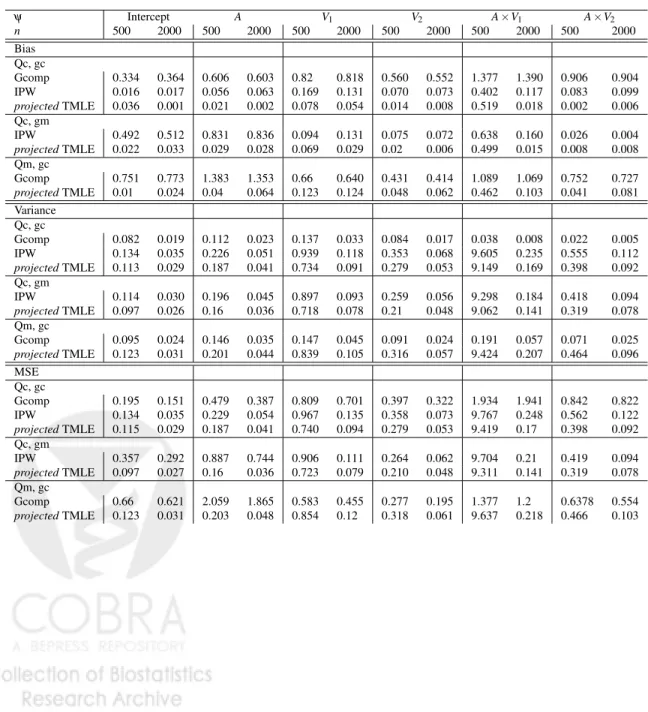
The bias, variance, and coverage probability (for the influence-function-based con-fidence intervals) are appraised using 500 repetitions.
In table 1, we see that when gA is misspecified, projected TMLE using a correct Qa
0
0,a1
t reduces bias over the misspecified IPW estimator. Similarly, when Qa
0
0,a1
t is misspecified, projected TMLE using the correctgA reduces bias over the
misspecified G-computation estimator. When comparing the correct vs misspec-ified G-computation estimators, and the correct vs misspecmisspec-ified IPW, coefficients involving the adjusted covariates (V1,V2) were still estimated very well by the
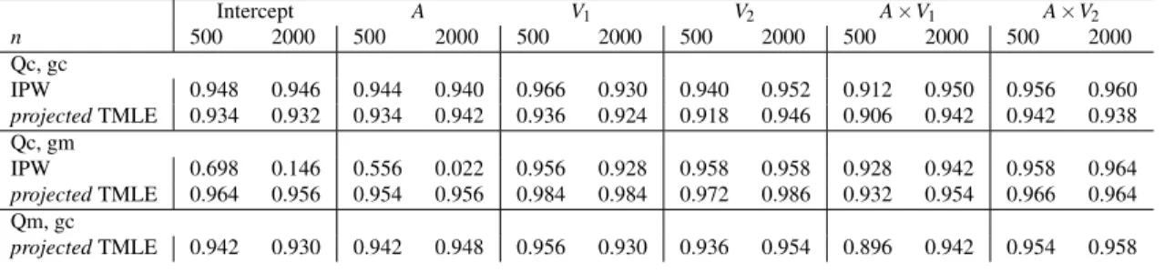
mis-specified estimator. Under ’Qc, gc’, the correct G-computation estimator converges much slower than the IPW and theprojectedTMLE estimators. We posit that this may be due to its sole reliance on the nonparametric likelihood estimates. As ex-pected, G-computation has the smallest sample variance, and IPW has the largest sample variance despite the truncated estimators for g. Under certain regularity
conditions, the IPW and projected TMLE estimators are asymptotically linear — table 2 tabulates the coverage probability of their Influence-Function based con-fidence intervals. At the correct models (Qc,gc), IPW and projected TMLE are asymptotically linear with influence functionDIPW andDA0, respectively. We used
p ˆ
varDIPWn /nand q
ˆ varDA0
n /nto estimate their respective standard errors. As
sam-ple size grows, the actual coverage probability is quite close to the nominal cover-age probability, with IPW having a better covercover-age. When one of the components is misspecified, theprojected TMLE still provides very good coverage, even though theoretically DA0 is only part of its influence curve; we postulate that this is
be-cause the influence function based standard error estimates are large relative to the finite sample bias. The misspecified IPW has very good coverage for the covari-ates that were adjusted for in the misspecified model, but very bad coverage for the confounded coefficients (Aand the intercept).
6
Data Analysis Example
To illustrate the application of theprojectedTMLE, we revisit our earlier example: the Sequenced Treatment Alternatives to Relieve Depression (STAR*D). After an initial screening process, patients are enrolled into level 1 of the treatment, where everyone was treated with citalopram. At the start of each subsequent level, if a patient still remains in the study, then he is randomized to an option (i.e. a par-ticular mediation) within one of his accepted treatment strategies (augmenting vs switching). Regular follow-up visits are conducted throughout each level. At each follow-up visit, covariates are collected, and the patient is subject to dropout, enter-ing remission, or moventer-ing onto next level.
In the field of depression research, there is very few literature concerning individual baseline characteristics that may differentially modify the effect of the treatment strategies. For this data analysis example, suppose at level 2 we wish to identify potential modifiers of the effect of switching medication vs augmenting medication on the chances of entering remission by the end of level 2. Because the strategies themselves are not randomized, this analysis is de facto equivalent to that of an observational study, and our estimators will correspondingly account for baseline and time-varying confounding. All candidate modifiers are a priori selected through a literature review of previous START*D publications. These co-variates are measured prior to the assignment of level 2 treatment, either at study screening, clinical visits or exit surveys at the end of level 1. Many of these can-didate modifiers are subject to missingness, often times due to missing visits and surveys, therein lies the need for the tools developed here. Our study population is the set of 1395 patients at level 2 who found medication strategies acceptable. Note
that because switching medication and augmenting medication are general treat-ment strategies that encompasses various treattreat-ment options (specific medications), for most patients these strategies are self-selected. Table 3 tabulates the events in level 2 by strategy received. Note that there are three strategies received, but we are only comparing switching medication vs augmenting medication. The data struc-ture was described in detail in section 2 as part of our running example.
We consider here two types of potential effect modifiers: some are mea-sured at screening and some are meamea-sured at exit of level 1. Table 4 summarizes percent of missingness, range, and scale of each effect modifier. Of all the candidate modifiers proposed by literature review, we exclude from our analysis the history of amphetamine use at baseline and history of drug abuse, since these two variables are missing for more than 70% of the patients. The multivariate nature of most of the effect modifiers underscores the need for projected TMLE. IfV is screening covariate, W includes all demographic variables and medical and psychiatric his-tory prior to enrollment; ifV is level 1 exit covariate, then we add toW variables summarizing number of visits, adherence to study protocol, and time spent in level 1.
The MSM is a generalized linear model with logit link. The linear predictor
φ(a00,a1,v) = (1,a1,v1, . . . ,vk,a1×v1, . . . ,a1×vk)andψ≡ ψ1,ψ2,ψ3,1, . . . ,ψ3,k,ψ4,1, . . . ,ψ4,k
∈ R2k+2for the categoricalVwithk+1 categories, andφ(a00,a1,v) = 1,a1,v,v2,a1×v,a1×v2
andψ ≡(ψ1,ψ2,ψ3,1,ψ3,2,ψ4,1,ψ4,2)∈R6for the semi-continuousV. The kernel
weights areh(a00,a1,V) =P0(A1=a1|V), to be estimated using Super Learner with
fitting algorithms glm, knnreg, nnetand bayesglm. The Super Learner will use 10-fold cross validation to select the best weighted combination of these fitting algorithms to estimateh(a00,a1,V). The initial estimators ofgandQa
0
0,a1
t adjust for
all baseline covariates and time-varying covariates with up to 2 time lag (each co-variate is coupled with its missingness indicator). We used Super Learner with the fitting algorithms glm, knnreg, nnet and bayesglm; each fitting algorithm is coupled with each of the following screening algorithms: Spearman correlation tests at significance levels 0.01, 0.05, 0.1, 0.2; ranking p-values from the correlation tests and take the topkvariables, wherekranges from 10 variables up to 30% of the total number of variables being considered, in increments of 20. The Super Learner selects the best linear combination of all screening-fitting couples.
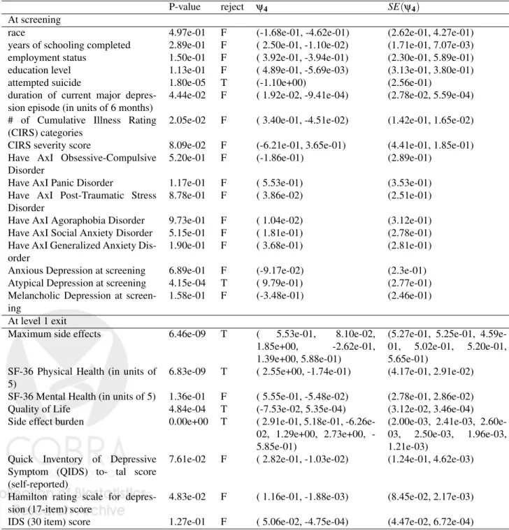
The goal of the analysis is to identify potential effect modifiers from a pool of candidate pre-treatment covariates. Our strategy is to measure the treatment heterogeneity for each of these covariates using an MSM, and then apply multiple hypothesis testing methods to identify those for which the treatment heterogeneity is significant. A common way to assess treatment heterogeneity across strata of V is to test whether the coefficients of the interaction terms ψ4= (ψ4,1, . . .ψ4,k)are
different from 0. We perform the corresponding Wald test in table 5, with the null hypothesis ψ4=0 and test statistics Tn=ψ4,n>Σn−1ψ4,n ∼χk2, where ψ4,n is the
A0−T MLE estimator,Σn=Covˆ (DAψ04)/n, andkis the number of interaction terms.
The false discovery rate (FDR) of the simultaneous comparisons are controlled at 0.05 with the Benjamini-Hochberg procedure.
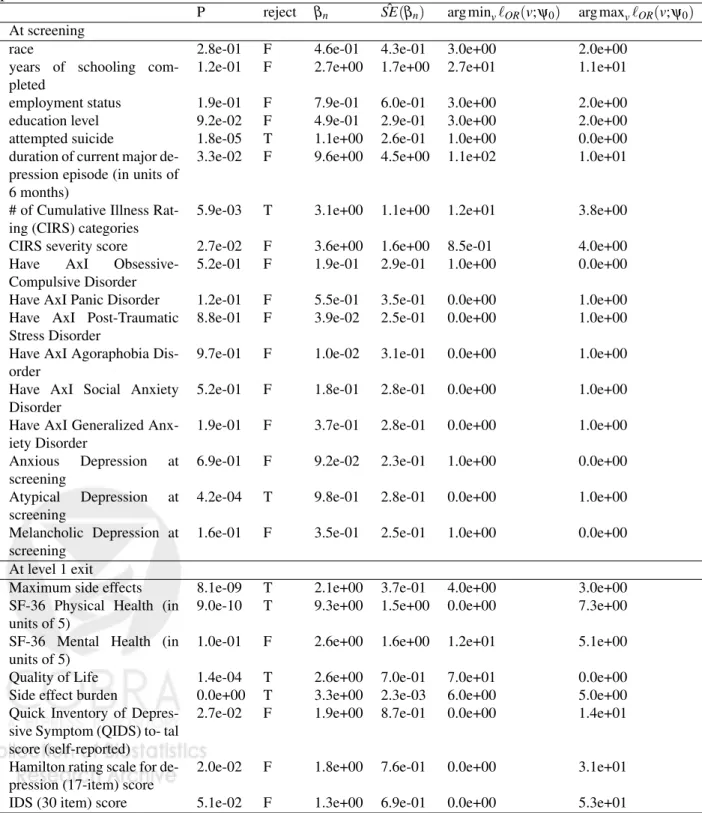
Since these candidate covariates differ in their type (semi-continuous vs bi-nary vs multiple categories), the corresponding MSM parameters are of different dimensions, we also consider the measure of treatment heterogeneity
β(ψ)≡max v `OR(v;ψ)−minv `OR(v;ψ), where `OR(v;ψ) =log m(1,v;ψ) 1−m(1,v;ψ)−log m((0,v;ψ) 1−m(0,v;ψ)= ( ψ2+ψ4,1v1+· · ·+ψ4,kvk, for categoricalV, ψ2+ψ4,1v+ψ4,2v2,for semi-continuousV.
This measure quantifies the most change in log odds ratio between any two val-ues ofV. Consider the null hypothesis H0 :β(ψ0) =0. Usingprojected TMLE,
we obtain an estimator βn=β(ψnpT MLE) of β0 for eachV. An application of the
functional delta Method, with the covariance matrixΣn of the estimated influence
functionDA0
n , yields a standard error estimateSEn forβn. We use the test statistics Tn=βn/SEn∼N(0,1). The results of the analysis are summarized in table 6.
In-terestingly, the two approaches yield almost all the same potential effect modifiers. Using our methods, we identified six factors, two at screening and four at level 1 exit, that modified the comparative treatment effect of augmenting vs switching medication. These effect modifiers are: prior suicide attempts, atypical depression, level 1 side-effect frequencies and burden (impairment), SF-36 phys-ical functionality, and quality of life at level 1 exit. In general, the heterogeneity of the treatment effects are most pronounced for the level 1 exit modifiers than for those from screening, indicating opportunities for close monitoring and medication management.
There has only been one publication that addressed the heterogeneous treat-ment effects between switching and augtreat-menting in level 2 treattreat-ment in STAR*D (Ellis, Dusetzina, Hansen, Gaynes, Farley, and Stumer (2013)). The authors em-ployed propensity score and weighting methods to examine heterogeneity of the treatment effect among the treated (medication augmentation) through stratifica-tion by propensity score decile. This approach does not explicitly identify factors contributing to heterogeneity. Missing data is less problematic in this case, and is handled by multiple imputation.
Table 1: Results: Bias, Variance, MSE for estimators ofψ0. Qc = correct Q a00,a1 t , Qm= misspecifiedQa 0 0,a1 t , gc=correctgA, gm=misspecifiedgA. ψ Intercept A V1 V2 A×V1 A×V2 n 500 2000 500 2000 500 2000 500 2000 500 2000 500 2000 Bias Qc, gc Gcomp 0.334 0.364 0.606 0.603 0.82 0.818 0.560 0.552 1.377 1.390 0.906 0.904 IPW 0.016 0.017 0.056 0.063 0.169 0.131 0.070 0.073 0.402 0.117 0.083 0.099 projectedTMLE 0.036 0.001 0.021 0.002 0.078 0.054 0.014 0.008 0.519 0.018 0.002 0.006 Qc, gm IPW 0.492 0.512 0.831 0.836 0.094 0.131 0.075 0.072 0.638 0.160 0.026 0.004 projectedTMLE 0.022 0.033 0.029 0.028 0.069 0.029 0.02 0.006 0.499 0.015 0.008 0.008 Qm, gc Gcomp 0.751 0.773 1.383 1.353 0.66 0.640 0.431 0.414 1.089 1.069 0.752 0.727 projectedTMLE 0.01 0.024 0.04 0.064 0.123 0.124 0.048 0.062 0.462 0.103 0.041 0.081 Variance Qc, gc Gcomp 0.082 0.019 0.112 0.023 0.137 0.033 0.084 0.017 0.038 0.008 0.022 0.005 IPW 0.134 0.035 0.226 0.051 0.939 0.118 0.353 0.068 9.605 0.235 0.555 0.112 projectedTMLE 0.113 0.029 0.187 0.041 0.734 0.091 0.279 0.053 9.149 0.169 0.398 0.092 Qc, gm IPW 0.114 0.030 0.196 0.045 0.897 0.093 0.259 0.056 9.298 0.184 0.418 0.094 projectedTMLE 0.097 0.026 0.16 0.036 0.718 0.078 0.21 0.048 9.062 0.141 0.319 0.078 Qm, gc Gcomp 0.095 0.024 0.146 0.035 0.147 0.045 0.091 0.024 0.191 0.057 0.071 0.025 projectedTMLE 0.123 0.031 0.201 0.044 0.839 0.105 0.316 0.057 9.424 0.207 0.464 0.096 MSE Qc, gc Gcomp 0.195 0.151 0.479 0.387 0.809 0.701 0.397 0.322 1.934 1.941 0.842 0.822 IPW 0.134 0.035 0.229 0.054 0.967 0.135 0.358 0.073 9.767 0.248 0.562 0.122 projectedTMLE 0.115 0.029 0.187 0.041 0.740 0.094 0.279 0.053 9.419 0.17 0.398 0.092 Qc, gm IPW 0.357 0.292 0.887 0.744 0.906 0.111 0.264 0.062 9.704 0.21 0.419 0.094 projectedTMLE 0.097 0.027 0.16 0.036 0.723 0.079 0.210 0.048 9.311 0.141 0.319 0.078 Qm, gc Gcomp 0.66 0.621 2.059 1.865 0.583 0.455 0.277 0.195 1.377 1.2 0.6378 0.554 projectedTMLE 0.123 0.031 0.203 0.048 0.854 0.12 0.318 0.061 9.637 0.218 0.466 0.103
Table 2: Coverage Probability for the Asymptotically Linear Estimators, using Influence-Function based Confidence Interval. Qc = correctQa
0 0,a1 t , Qm= misspeci-fiedQa 0 0,a1 t , gc=correctgA, gm=misspecifiedgA. Intercept A V1 V2 A×V1 A×V2 n 500 2000 500 2000 500 2000 500 2000 500 2000 500 2000 Qc, gc IPW 0.948 0.946 0.944 0.940 0.966 0.930 0.940 0.952 0.912 0.950 0.956 0.960 projectedTMLE 0.934 0.932 0.934 0.942 0.936 0.924 0.918 0.946 0.906 0.942 0.942 0.938 Qc, gm IPW 0.698 0.146 0.556 0.022 0.956 0.928 0.958 0.958 0.928 0.942 0.958 0.964 projectedTMLE 0.964 0.956 0.954 0.956 0.984 0.984 0.972 0.986 0.932 0.954 0.966 0.964 Qm, gc projectedTMLE 0.942 0.930 0.942 0.948 0.956 0.930 0.936 0.954 0.896 0.942 0.954 0.958
Table 3: Level 2 events by acceptable strategy received Med-Sw Med-Aug any CT
Received 727 565 103
Success 257 (35%) 287 (51%) 53 (51%) No Success 227 (32%) 132 (23%) 22 (21%) Dropout 243 (33%) 146 (26%) 28 (27%)
Table 4: Candidate effect modifiers of interest for level 2. Candidates with more than 50% missing in the study population will be discarded from the analysis.
% missing type (# of categories, or range of semi-continuous variable)
At screening
race 0 Categorical (3)
years of schooling completed 0 Semi-continuous (0,27)
employment status 0 Categorical (3)
education level 0 Categorical (3)
attempted suicide 0 Categorical (2)
duration of current major depression episode (in units of 6 months)
1 Semi-continuous (0,111)
AxI: Amphetamine 73 (will not use) Categorical (2)
history of drug abuse 76 (will not use) Categorical (2)
# of Cumulative Illness Rating (CIRS) categories 0 Semi-continuous (0,12)
CIRS severity score 0 Semi-continuous (0,4)
Have AxI Obsessive-Compulsive Disorder 1 Categorical (2)
Have AxI Panic Disorder 1 Categorical (2)
Have AxI Post Traumatic Stress Disorder 2 Categorical (2)
Have AxI Agoraphobia 1 Categorical (2)
Have AxI Social Anxiety Disorder 2 Categorical (2)
Have AxI Generalized Anxiety Disorder 2 Categorical (2)
Anxious Depression at screening 6 Categorical (2)
Atypical Depression at screening 5 Categorical (2)
Melancholic Depression at screening 5 Categorical (2) At level 1 exit
Maximum Side Effects 1 Categorical (7)
SF-36 Physical Health (in units of 5) 23 Semi-continuous (0,12) SF-36 Mental Health (in units of 5) 23 Semi-continuous ((0,12)
Quality of Life 23 Semi-continuous (0,98)
Side effect burden 1 Categorical (7)
Quick Inventory of Depressive Symptom (QIDS) total score (self-reported)
1 Semi-continuous (0,27) Hamilton rating scale for depression (17-time) score 12 Semi-continuous (0,43)
Table 5: Data Analysis Results: Multivariate Wald Test. ψ4= (ψ4,1, . . .ψ4,k) are
the coefficients of the interaction terms in the MSM; ifV is semi-continuous, in-teraction terms areψ4·(v,v2), ifV is categorical withk+1 categories, interaction
terms areψ4·(v1, . . . ,vk). H0:ψ4=0.Tn=ψ4,n>Σ−n1ψ4,n∼χk2, whereψnis given
by projected TMLE, and Σn is the corresponding covariance estimator based on
the covariance matrix of the projected-IC. Control false discovery rate at 0.05 with Benjamini-Hochberg procedure
P-value reject ψ4 SE(ψ4)
At screening
race 4.97e-01 F (-1.68e-01, -4.62e-01) (2.62e-01, 4.27e-01)
years of schooling completed 2.89e-01 F ( 2.50e-01, -1.10e-02) (1.71e-01, 7.07e-03) employment status 1.50e-01 F ( 3.92e-01, -3.94e-01) (2.30e-01, 5.89e-01) education level 1.13e-01 F ( 4.89e-01, -5.69e-03) (3.13e-01, 3.80e-01)
attempted suicide 1.80e-05 T (-1.10e+00) (2.56e-01)
duration of current major depres-sion episode (in units of 6 months)
4.44e-02 F ( 1.92e-02, -9.41e-04) (2.78e-02, 5.59e-04) # of Cumulative Illness Rating
(CIRS) categories
2.05e-02 F ( 3.40e-01, -4.51e-02) (1.42e-01, 1.65e-02) CIRS severity score 8.09e-02 F (-6.21e-01, 3.65e-01) (4.41e-01, 1.85e-01) Have AxI Obsessive-Compulsive
Disorder
5.20e-01 F (-1.86e-01) (2.89e-01)
Have AxI Panic Disorder 1.17e-01 F ( 5.53e-01) (3.53e-01) Have AxI Post-Traumatic Stress
Disorder
8.78e-01 F ( 3.86e-02) (2.51e-01)
Have AxI Agoraphobia Disorder 9.73e-01 F ( 1.04e-02) (3.12e-01) Have AxI Social Anxiety Disorder 5.15e-01 F ( 1.81e-01) (2.78e-01) Have AxI Generalized Anxiety
Dis-order
1.90e-01 F ( 3.68e-01) (2.81e-01)
Anxious Depression at screening 6.89e-01 F (-9.17e-02) (2.3e-01) Atypical Depression at screening 4.15e-04 T ( 9.79e-01) (2.77e-01) Melancholic Depression at
screen-ing
1.58e-01 F (-3.48e-01) (2.46e-01)
At level 1 exit
Maximum side effects 6.46e-09 T ( 5.53e-01, 8.10e-02, 1.85e+00, -2.62e-01, 1.39e+00, 5.88e-01)
(5.27e-01, 5.25e-01, 4.59e-01, 5.02e-01, 5.20e-01, 5.65e-01)
SF-36 Physical Health (in units of 5)
6.83e-09 T ( 2.55e+00, -1.74e-01) (4.17e-01, 2.91e-02) SF-36 Mental Health (in units of 5) 1.36e-01 F ( 5.55e-01, -5.48e-02) (2.78e-01, 2.86e-02) Quality of Life 4.84e-04 T (-7.53e-02, 5.35e-04) (3.12e-02, 3.46e-04) Side effect burden 0.00e+00 T ( 2.91e-01, 5.18e-01,
6.26e02, 1.29e+00, 2.73e+00, -5.85e-01)
(2.00e-03, 2.41e-03, 2.60e-03, 2.50e-03, 1.96e-03, 1.21e-03)
Quick Inventory of Depressive Symptom (QIDS) to- tal score (self-reported)
Table 6: Data Analysis Results:β0=maxv`OR(v;ψ0)−minv`OR(v;ψ0),H0:β0=0.
Tn=βn/SEn∼N(0,1), whereψngiven byprojectedTMLE. The standard error
es-timate ˆSE(βn)is computed using on the variance of the projected-IC and the
func-tional delta method. Control false discovery rate at 0.05 with Benjamini-Hochberg procedure
P reject βn SE(ˆ βn) arg minv`OR(v;ψ0) arg maxv`OR(v;ψ0)
At screening
race 2.8e-01 F 4.6e-01 4.3e-01 3.0e+00 2.0e+00
years of schooling com-pleted
1.2e-01 F 2.7e+00 1.7e+00 2.7e+01 1.1e+01 employment status 1.9e-01 F 7.9e-01 6.0e-01 3.0e+00 2.0e+00
education level 9.2e-02 F 4.9e-01 2.9e-01 3.0e+00 2.0e+00
attempted suicide 1.8e-05 T 1.1e+00 2.6e-01 1.0e+00 0.0e+00 duration of current major
de-pression episode (in units of 6 months)
3.3e-02 F 9.6e+00 4.5e+00 1.1e+02 1.0e+01
# of Cumulative Illness Rat-ing (CIRS) categories
5.9e-03 T 3.1e+00 1.1e+00 1.2e+01 3.8e+00 CIRS severity score 2.7e-02 F 3.6e+00 1.6e+00 8.5e-01 4.0e+00 Have AxI
Obsessive-Compulsive Disorder
5.2e-01 F 1.9e-01 2.9e-01 1.0e+00 0.0e+00 Have AxI Panic Disorder 1.2e-01 F 5.5e-01 3.5e-01 0.0e+00 1.0e+00 Have AxI Post-Traumatic
Stress Disorder
8.8e-01 F 3.9e-02 2.5e-01 0.0e+00 1.0e+00 Have AxI Agoraphobia
Dis-order
9.7e-01 F 1.0e-02 3.1e-01 0.0e+00 1.0e+00 Have AxI Social Anxiety
Disorder
5.2e-01 F 1.8e-01 2.8e-01 0.0e+00 1.0e+00 Have AxI Generalized
Anx-iety Disorder
1.9e-01 F 3.7e-01 2.8e-01 0.0e+00 1.0e+00 Anxious Depression at
screening
6.9e-01 F 9.2e-02 2.3e-01 1.0e+00 0.0e+00 Atypical Depression at
screening
4.2e-04 T 9.8e-01 2.8e-01 0.0e+00 1.0e+00 Melancholic Depression at
screening
1.6e-01 F 3.5e-01 2.5e-01 1.0e+00 0.0e+00 At level 1 exit
Maximum side effects 8.1e-09 T 2.1e+00 3.7e-01 4.0e+00 3.0e+00 SF-36 Physical Health (in
units of 5)
9.0e-10 T 9.3e+00 1.5e+00 0.0e+00 7.3e+00 SF-36 Mental Health (in
units of 5)
1.0e-01 F 2.6e+00 1.6e+00 1.2e+01 5.1e+00
Quality of Life 1.4e-04 T 2.6e+00 7.0e-01 7.0e+01 0.0e+00
Side effect burden 0.0e+00 T 3.3e+00 2.3e-03 6.0e+00 5.0e+00 Quick Inventory of
Depres-sive Symptom (QIDS) to- tal score (self-reported)
7
Summary
In this work, we studied causal effect modification by a counterfactual modifier. The tools developed here are applicable in situations where the effect modifier of interest may be better cast as counterfactual variables. Examples of such situations include the study of time-varying effect modification, or the study of baseline ef-fect modification with modifiers that are missing at random. We established the efficient influence function (EIC) for the corresponding marginal structural model parameters which provides the semiparametric efficiency bound for all the asymp-totically linear estimators. This efficient influence function is also doubly robust in that it remains an unbiased estimating function if either 1) the outcome expecta-tions and the modifier density, or 2) the treatment and censoring mechanisms, are consistently estimat