UW Biostatistics Working Paper Series
11-28-2005
Optimal Feature Selection for Nearest Centroid
Classifiers, With Applications to Gene Expression
Microarrays
Alan R. Dabney
University of Washington, [email protected]
John D. Storey
University of Washington, [email protected]
This working paper is hosted by The Berkeley Electronic Press (bepress) and may not be commercially reproduced without the permission of the
Suggested Citation
Dabney, Alan R. and Storey, John D., "Optimal Feature Selection for Nearest Centroid Classifiers, With Applications to Gene Expression Microarrays" (November 2005).UW Biostatistics Working Paper Series.Working Paper 267.
Optimal Feature Selection for Nearest Centroid Classifiers, With
Applications to Gene Expression Microarrays
Alan R. Dabney and John D. Storey Department of Biostatistics
University of Washington, Seattle, WA 98195
[email protected],[email protected] October 2005
Abstract
Nearest centroid classifiers have recently been successfully employed in high-dimensional applications. A necessary step when building a classifier for high-dimensional data is feature selection. Feature selection is typically carried out by computing univariate statistics for each feature individually, without consideration for how a subset of features performs as a whole. For subsets of a given size, we characterize the optimal choice of features, corresponding to those yielding the smallest misclassification rate. Furthermore, we propose an algorithm for estimating this optimal subset in practice. Finally, we investigate the applicability of shrinkage ideas to nearest centroid classifiers. We use gene-expression microarrays for our illustrative examples, demonstrating that our proposed algorithms can improve the performance of a nearest centroid classifier.
1
Introduction
Linear Discriminant Analysis (LDA) is a long-standing prediction method that has been well char-acterized when the number of features used for prediction is small (Mardia et al. 1979). The method has recently been shown to compare favorably with more complicated classifiers in high-dimensional applications, where there are thousands of potential features to employ, but only a subset are used (Dudoit et al. 2002, Tibshirani et al. 2002, Lee et al. 2005). In the LDA setting, each class is characterized by its vector of average feature values (i.e., class centroid). A new observation is evaluated by computing the scaled distance between its profile and each class centroid. The ob-servation is then assigned to the class to which it is nearest, allowing LDA to be interpreted as a “nearest centroid classifier.”
In high-dimensional applications, it is often desirable to build a classifier using only a subset of features due to the fact that (1) many of the features are not informative for classification and (2) the number of training samples available for building the classifier is substantially smaller than the number of possible features. In any case, it could be argued that a classifier built with a smaller number of features is preferable to an equally accurate classifier built with the complete set of features. Several approaches have been proposed for nearest centroid classifiers that rely on univariate statistics for feature selection (Golub et al. 1999, Hedenfalk et al. 2001, Dudoit et al. 2002, Tibshirani et al. 2002). These methods assess each feature individually by its ability to discriminate the classes. However, it has been noted that the features that best discriminate the classes individually are not necessarily the ones that work besttogether(Jaeger et al. 2003, Dabney 2005).
In the extremely simple case where features are uncorrelated and only two classes exist, it intuitively follows that the optimal set of features are those whose means are most different between
the two classes. However, this intuition does not easily carry over to the more complicated (and topical) case where features are correlated and/or there are more than two classes. For example, if we seek to classify among three classes, it has not been shown whether it is better to choose features that distinguish one class from the other two well or those that distinguish among all three classes well. The role of correlation between features is not currently well understood either.
In this paper, we show how to exactly choose the subset of features of a given size that mini-mizes the misclassification rate. This optimal feature set takes into account the joint behavior of the features in two ways. First, it explicitly incorporates information about correlation between features. Second, it assesses how a group of features as a whole is capable of distinguishing be-tween multiple classes. Overall, it eliminates the need for heuristically-motivated feature selection criteria in high-dimensional settings, and shows one exactly what the optimal solution is. That is, our main theoretical result allows one to directly aim for the optimal choice. However, one must then estimate the optimal choice of features in practice, for which we propose a greedy algorithm and demonstrate its operating characteristics.
Finally, we investigate the application of shrinkage ideas to the classification problem. Shrinkage of multivariate estimates is known to improve their overall accuracy. It has also been suggested that shrinkage can improve nearest centroid classifiers (Tibshirani et al. 2002). However, the shrinkage approach taken in Tibshirani et al. (2002) tends to actually increase misclassification error (Dabney 2005), leaving the question of shrinkage in classifiers open. We show that shrinkage can, in principle, improve classification. Furthermore, we propose a novel shrinkage procedure for nearest centroid classifiers.
Nearest centroid classifiers have been shown to perform well with gene-expression microarrays (Dudoit et al. 2002, Lee et al. 2005, Tibshirani et al. 2002, Dabney 2005), and we illustrate our
findings in this setting. We compare our proposed method with existing nearest centroid classifiers on four previously-published microarray datasets, demonstrating that improvements in prediction accuracy can be attained by estimating the optimal feature-selection criteria (Figure 2). Our estimated optimal-feature selection algorithm can be further improved by employing our shrinkage procedure (Figure 2).
2
Linear Discriminant Analysis (LDA)
The problem LDA addresses is to classify unknown samples into one of K classes. To build a classifier, we obtain nk training samples per class, k = 1,2, . . . , K, with m features per sample. For each training sample, we observe class membership Y and profile X. For simplicity, we will represent the classes by the numbers 1,2, . . . , K. Note that each profile is a vector of lengthm. We assume that profiles from classkare distributed asN(µk,Σ), the multivariate normal distribution with mean vector µk and covariance matrix Σ. Call L(·; µk,Σ) the corresponding probability density function. Finally, letπk be the prior probability that an unknown sample comes from class
k,k= 1,2, . . . , K.
Bayes’ Theorem states that the probability that an observed sample comes from class k is proportional to the product of the class density and prior probability:
Pr(Y =k|X =x)∝L(x; µk,Σ)×πk. (a)
to the class with the largest posterior probability:
ˆ
y= argmaxk{L(x; µk,Σ)×πk}. (b)
This can be shown to be the rule that minimizes misclassification error (Mardia et al. 1979). We can rewrite (b) as
ˆ
y = argmink
(x−µk)TΣ−1(x−µk)−2 log(πk) . (c)
Thus, a sample is assigned to the class to which it is nearest, as measured by the metric kx−
µk2
Σ−2 log(π), where kx−µk2Σ= (x−µ)TΣ
−1(x−µ) is the square of the Mahalanobis distance
betweenxand µ.
3
Optimal Subsets in Theory
Misclassification rates. A misclassification occurs when a sample is assigned to the incorrect class. The probability of making a classification error is:
Pr(error) = K X j=1 h Pr( ˆY 6=j|Y =j)×πj i .
We can derive misclassification rates using the LDA rule (c). In particular, we can calculate mis-classification rates for any subset of features. An optimal subset can be found by simply assigning misclassification rates to all possible subsets of a given size and choosing the one with the lowest error rate. Lemma 1 characterizes misclassification rates for a set of centroids, Theorem 1
de-scribes how to find the optimal subset of a given size, and the Remark shows a simplified result corresponding to equal prior probabilities.
Lemma 1 Suppose that a sample from classkis distributed according toNm(µk,Σ),k= 1,2, . . . , K.
Let πk be the prior probability that a sample comes from class k, k= 1,2, . . . , K. The
misclassifi-cation rate of a nearest-centroid (LDA) classifier is
Pr(error) = K X j=1 (" 1−φmin i6=j ( kµj−µik2Σ+ 2 log( πj πi) 2kµj−µikΣ ) # ×πj ) , (d)
where φis the cdf of the standard normal distribution, and kµj−µik2Σ= (µj−µi)TΣ−1(µj−µi)
is the square of the Mahalanobis distance between µj andµi.
This allows us to state the following theorem showing how to determine the optimal subset of features of sizem0 for LDA classification.
Theorem 1 (LDA Optimal Subset Selection) Under the setting described in Lemma 1, the subset of features of sizem0≤mthat minimizes the misclassification rate is the one with the lowest value of equation (d). Remark 1 If π1=π2 =. . .=πK, then Pr(error) = 1 K K X j=1 1−φ min i6=j 1 2kµj−µikΣ .
A subset of features can be evaluated using (d), where only the subset of features are included in the centroids. Note that equation (d) can be interpreted as measuring the collective distance between all of the class centroids. In general, the misclassification rate will be small when all of the class
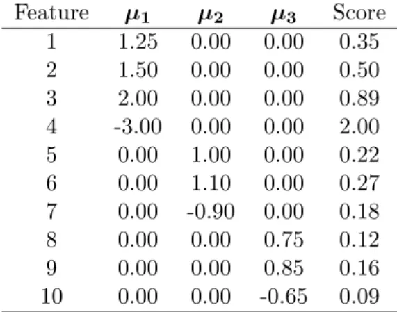
Table 1: Simulated class means with 10 features and 3 classes. Feature µ1 µ2 µ3 Score 1 1.25 0.00 0.00 0.35 2 1.50 0.00 0.00 0.50 3 2.00 0.00 0.00 0.89 4 -3.00 0.00 0.00 2.00 5 0.00 1.00 0.00 0.22 6 0.00 1.10 0.00 0.27 7 0.00 -0.90 0.00 0.18 8 0.00 0.00 0.75 0.12 9 0.00 0.00 0.85 0.16 10 0.00 0.00 -0.65 0.09
centroids are far away from each other. Note, however, that the score in (d) is actually a complicated combination of the pairwise differences between the centroids and the class priors. Furthermore, correlations between features are explicitly incorporated through the distance functionskµj−µikΣ,
i6=j. Further intuition into (d) can be attained by considering the following simple example.
A Simple Example. The data in Table 1 represent a simulated example with 10 features and 3 classes. The population means of each class are shown in columns two through four; we assume that each feature has variance 0.5 and that all features are uncorrelated. Suppose that we wish to select the five features that correspond to the lowest misclassification error. The final column of the table lists univariate scores for each feature, where we have used the average squared difference from the feature mean as the score. A high value for a feature on this score indicates large overall differences between this feature’s class means. The five largest univariate scores correspond to features 1, 2, 3, 4, and 6.
An alternative approach to using univariate scores to select features is to consider all 105= 252 possible quintuplets and choose the set with the lowest overall misclassification rate. Note that, to do this, we must be able to assign misclassification probabilities to arbitrary feature subsets.
This highlights the novelty and usefulness of the multivariate score (d). Using (d), we find that the set of features chosen by the univariate scores has an overall misclassification rate of 15%. Similarly, we find that the optimal set in this example contains features 4, 5, 6, 7, and 9, with an associated error rate of 6%. The most obvious difference between this subset and that chosen by univariate scores is the exclusion of features 1, 2, and 3. Apparently, class one can be sufficiently characterized by feature 4. The other features do not contain sufficient additional information to merit their selection.
Correlation between features. An important aspect of the optimal feature-selection procedure is its explicit incorporation of correlation between features. It is not necessarily clear what effect correlation between features should have on a classifier. Some have argued that it is inefficient to select correlated features (Jaeger et al. 2003). Bickel & Levina (2004) show that estimating correlations as zero can lead to better prediction when the number of features is large relative to the number of samples. Meanwhile, recent optimality results in the context of multiple hypothesis testing (Storey 2005, Storey et al. 2005) suggest that correlated features may be beneficial in distinguishing groups. Intuitively, many weakly informative, correlated genes might be expected to collectively be highly informative.
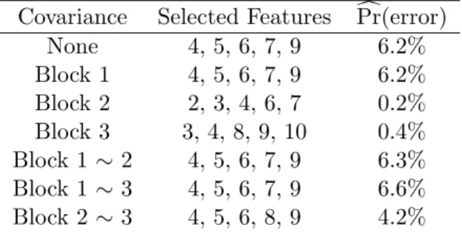
We briefly investigate the effect of different correlation patterns in the example of Table 1. Let Σbe the 10×10 covariance matrix. In Table 2, we refer to the 4×4 diagonal block corresponding to features 1−4 as “Block 1.” The diagonal blocks corresponding to features 5−7 and 8−10 are similarly referred to as “Block 2” and “Block 3.” “Block 1∼2” refers to the off-diagonal block relating features 1−4 to features 5−6,etc.. In all cases, we include a common pairwise correlation of 0.9; no qualitative differences were found when considering negative correlation.
Table 2: The effect of covariance on the optimal feature-selection procedure. Covariance Selected Features Pr(error)c
None 4, 5, 6, 7, 9 6.2% Block 1 4, 5, 6, 7, 9 6.2% Block 2 2, 3, 4, 6, 7 0.2% Block 3 3, 4, 8, 9, 10 0.4% Block 1∼2 4, 5, 6, 7, 9 6.3% Block 1∼3 4, 5, 6, 7, 9 6.6% Block 2∼3 4, 5, 6, 8, 9 4.2%
In this example, correlation between features in Blocks 2 and 3 has the largest effect, on both the optimal set of features and the probability of misclassification. The features in Blocks 2 and 3 are individually less informative than those in Block 1. Note, in particular, that when the features in Block 3 are correlated, all three components are selected, whereas only one is selected in the absence of correlation. These results suggest that correlated features can be useful together, particularly when the correlated features contain relatively little information individually. More generally, there are many possible scenarios in which correlation could play a role. The main point is that the feature-selection procedure (d) automatically identifies the optimal combination of features, even in the presence of correlation.
4
Optimal Subsets in Practice
Often, there will be many more than 10 features from which to choose. With gene expression microarrays, for example, there are thousands of genes under consideration. Thus, in practice, it may be impossible to perform an exhaustive search for a best subset. Even if we could perform an exhaustive search, we would still need to estimate the class centroids, and this may not lead to the correct solution. We propose a greedy algorithm for estimating the optimal subset of given size
when an exhaustive search is not possible. We compare our algorithm with a more conventional univariate scoring algorithm for choosing subsets on both simulated (Figure 1) and real (Figure 2) datasets.
Univariate Scoring Procedures. The novelty of our proposed method can better be understood by first considering some of the available methods for choosing features, which are all based on univariate scoring of features. An early suggestion in the context of gene expression microarrays usedF-statistics to evaluate each feature (here, a gene) individually on the basis of comparisons of between-class variation and within-class variation (Dudoit et al. 2002):
Fi = BSS W SS = Pn j=1 PK k=1I(yj =k)(ˆµik−µˆi)2 Pn j=1 PK k=1I(yj =k)(xij−µˆik)2 ,
i= 1,2, . . . , m. To form a classifier using only ˜m features, class centroids are formed with only the features corresponding to the largest ˜m F-statistics. All other features are discarded.
Another example (again in the context of microarrays) is Prediction Analysis of Microarrays (PAM) (Tibshirani et al. 2002). Instead ofF-statistics, PAM uses the statistics
dik= ˆ
µik−µˆi
wk(si+s0)
to select genes, wheresi is the pooled standard deviation for featurei,wk= (1/nk−1/n)1/2 makes
wk×si equal to the standard error of the numerator, and s0 is a fudge factor intended to guard
against very large statistics for very small standard errors. Withouts0,dikis at-statistic comparing the mean of featureiin classkto the overall mean of feature i. Hence, dik measures the difference between feature i in class k and feature i in all classes combined. PAM then shrinks the dik’s
toward zero, eliminating the features that do not provide sufficient discriminatory information. The Classification to Nearest Centroids (ClaNC) method (Dabney 2005) uses simple t-statistics without fudge factors or shrinkage and outperforms PAM on both simulated and real datasets.
Algorithm for Estimating the Optimal Solution. When it is not feasible to perform an exhaustive search for the best subset of features of a given size, we propose the following greedy algorithm. Letsbe the indices of a subset of features, and let µs denote a centroid indexed by s. Define the estimated scoring function to be
d Pr(error ; s) = K X j=1 (" 1−φmin i6=j ( kµˆsj−µˆsik2 ˆ Σ+ 2 log( πj πi) 2kµˆsj−µˆsikΣˆ ) # ×πj ) . (e)
1. Evaluate all m features individually using (e), and select the first feature to be the one with the lowest score. This leavesm−1 features from which to choose.
2. Combine each remaining feature with the one already chosen and compute the m−1 scores corresponding to each invidual pair.
3. Choose the second feature to be the one that produces the lowest score when combined with the first.
4. Continue this process until the desired number of features have been selected.
Note thatΣˆ in (e) is a matrix of estimated covariances. As we saw with the examples in Tables 1 and 2, classification accuracy can be improved by incorporating correlation between features. However, in high-dimensional settings, it may be impractical and/or unnecessary (Bickel & Levina 2004) to estimate large covariance matrices for large numbers of features. This is one motivation behind shrinking covariances to zero when building classifiers for microarrays. In the microarray
examples below, the classifiers we present do not include estimated covariances. There was no gain in accuracy in these examples when estimating covariances by maximum likelihood (results not shown). This could either mean covariances are truly irrelevant in these examples, or that our covariance estimates are imprecise. In future work, we plan to investigate the utility of shrinkage estimates of the covariance matrix; it is desirable to include such information, since it is fully characterized by Theorem 1.
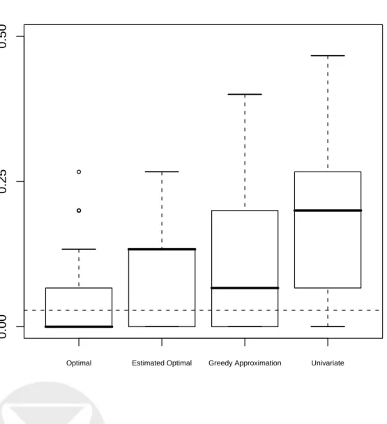
Illustration on Simulated Example. For each of 50 simulations, we generated random ob-servations from the setting described in Table 1, assuming a common pairwise correlation of 0.5 within each of Blocks 1, 2, and 3, as described in Table 2. In each simulation, 15 training samples (five per class) and 15 test samples (again, five per class) were generated. We then compared the misclassification rates (computed on the test data) after selecting subsets of size five in different ways (on the training data), with the results shown as boxplots in Figure 1. Our standard of comparison was the classifier built using the optimal subset found above, labeled “Optimal.” We also carried out an exhaustive search for the optimal subset in each simulation; these results are labeled “Estimated Optimal.” “Greedy Approximation” refers to the algorithm described above. Finally, the “Univariate” results correspond to choosing subsets based on univariate scores. In this comparison, we used the F-statistic approach of Dudoit et al. (2002).
Figure 1 about here.
The true optimal subset of size five produces the most accurate classifier, as expected. The exhaus-tive search apparently did not identify the true optimal subset, although its choice was superior to that made by the univariate scoring procedure. The greedy algorithm estimates the optimal feature subset well in this example.
Illustration on Real Examples. We now illustrate our methods on four previously published gene-expression microarray experiments. In each analysis, any missing values were imputed using
K-nearest-neighbors (Troyanskaya et al. 2001) withK = 10. We compare the methods on the basis of error rates from five-fold cross-validation. We avoid gene-selection bias by completely rebuilding classifiers to identical specifications in each cross-validation iteration (Ambroise & McLachlan 2002). Cross-validated error rates are nearly unbiased, being slightly conservative (Ambroise & McLachlan 2002, Hastie et al. 2001), and they are thus sufficient for comparing classifiers.
The first example involves small round blue cell tumors (SRBCT) of childhood (Khan et al. 2001). Expression measurements were made on 2,307 genes in 83 SRBCT samples. The tumors were classified as Burkitt lymphoma, Ewing sarcoma, neuroblastoma, or rhabdomyosarcoma. There are 11, 29, 18, and 25 samples in each respective class. In the second example, expression mea-surements were made on 4,026 genes in 58 lymphoma patients (Alizadeh et al. 2000). The tumors were classified as diffuse large B-cell lymphoma and leukemia, follicular lymphoma, and chronic lymphocytic leukemia. There are 42, 6, and 10 samples in each respective class. The third example involves the cell lines used in the National Cancer Institute’s screen for anti-cancer drugs (Ross et al. 2000, Scherf et al. 2000). Expression measurements were made on 6,830 genes in 60 cell tu-mors. There are representative cell lines for each of lung cancer, prostate cancer, CNS, colon cancer, leukemia, melanoma, NSCLC, ovarian cancer, renal cancer, and one unknown sample. We filtered out 988 genes for which 20% or more of the tumors had missing values. We also excluded samples from prostate cancer (due to there being only two samples) and the one unknown sample. There are 9, 6, 7, 6, 8, 7, 6, and 8 samples in each remaining respective class. The fourth example involves acute myeloid leukemia (AML) and acute lymphblastic leukemia (ALL) (Golub et al. 1999). The public version of the training data used in the original analysis include expression measurements
on 3,857 genes in 38 leukemia patients. There are 11 and 27 samples in each respective class. Figure 2 about here.
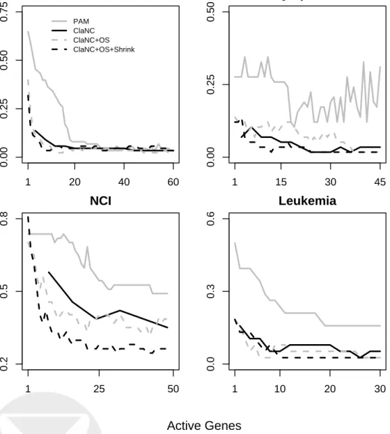
Figure 2 shows misclassification rates for a variety of subset sizes. The estimated optimal subsets using the algorithm described above compare favorably with both PAM and ClaNC. That is, for any given number of active features, classifiers built with estimated optimal subsets have error rates that tend to be smaller than (or equal to) those for PAM or ClaNC.
Shrinkage. As mentioned earlier, the LDA classification rule minimizes the misclassification rate, because the LDA rule equals the Bayes’ rule under its assumptions (Mardia et al. 1979). For simplicity in motivating shrinkage, assume all features are independent with variance one, and that each class has equal prior probability. Then the Bayes’ rule is to classify a new sample to the class for which Pm
i=1(x ∗
i −µik)2 is smallest. However, we must estimate the centroids µk in practice, using µˆk in their place. Suppose x∗ comes from class k0. Then, expanding the squared distance
betweenx∗ to class k0 and taking expectations, we have
E m X i=1 (x∗i −µˆik0) 2 = E m X i=1 (x∗i −µik0 +µik0 −µˆik0) 2 = E m X i=1 (x∗i −µik0) 2+ E m X i=1 (µik0 −µˆik0) 2, (f)
or the Bayes’ rule plus the mean squared error (MSE) of the centroid estimate.
Reducing the MSE of µˆk0 will bring us closer to the Bayes’ rule. According to Stein’s Paradox of statistics (Stein 1956), we can reduce the MSE of µˆk0 by shrinking towards the overall mean
Pm
i=1µˆik/m(or any other constant). In our setting, this suggests shrinking each centroid across its
m components. The PAM method (Tibshirani et al. 2002) incorporates shrinkage ideas. However, PAM shrinks each feature across classes. Since this makes the estimated class centroids more similar
to one another, the shrinkage employed by PAM appears to actually increase misclassification error (Dabney 2005). We now investigate whether shrinking centroids across features can improve classification.
While there are many possible approaches to shrinking the centroids, we take the following simple approach. Let µˆok be the m-vector with each component equal to ˆµok =Pm
i=1µˆik/m, k =
1,2, . . . , K. We consider shrunken centroids of the form
˜
µk=ωkµˆok+ (1−ωk)µˆk, (g)
k= 1,2, . . . , K. We chooseωk so that E(kµk−µ˜kk2Σ) is minimized, k= 1,2, . . . , K. Theorem 2 presents a general result, and the Corollary translates this result to the ideal case where all genes are independent.
Theorem 2 Let the maximum likelihood estimates of the class centroids be µˆk and µˆok be the m -vector with each component equal to the estimated overall mean for classk, k= 1,2, . . . , K. Among all estimators of the formµ˜k =ωkµˆok+ (1−ωk)µˆk, the error measure E(kµk−µ˜kk2Σ)is minimized
by choosing ˆ ωk = VΣ(µˆk)−CΣ(µˆk, µˆok) (µ¯k−µk)TΣ−1(µ¯ k−µk) +VΣ(µˆk) +VΣ(µˆok)−2CΣ(µˆk, µˆok) ,
where µ¯k is the m-vector with each component equal to µ¯k = m1 Pmi=1µik, VΣ(µˆk) = E(µˆk −
µk)TΣ−1(µˆ
k−µk),VΣ(µˆok) =E(µˆko−µ¯k)TΣ−1(µˆok−µ¯k), andCΣ(µˆk,µˆok) =E(µˆk−µk)TΣ−1(µˆok−
¯
Corollary 1 Assuming all genes are independent, ˆ ωk= m−1 nk Pm i=1 (¯µk−µik)2 σ2 i +m−2 + (m1 Pm i=1σ12 i )(m1 Pm i=1σ2i) , k= 1,2, . . . , K.
In practice, we use plug-in estimates for the unknown parameters.
Figure 2 also illustrates the performance of classifiers with estimated optimal subsets and shrunken centroids. The shrinkage was carried out on the complete centroids, prior to the feature-selection step. Another alternative would be to shrink the centroids of each considered feature subset individually. No qualitative differences were found when employing this shrinkage approach (results not shown). Improvements are evident over the other classifiers under consideration. This suggests that shrinkage can be successfully applied to nearest centroid classifiers and is worth further exploration.
5
Proofs of Theorems
Proof of Lemma 1. We begin with the simple two-class case. A classification error is made if we either predict class two for a sample that truly comes from class one or predict class one for a sample that truly comes from class two. That is,
Consider the first component of this sum. We can rewrite it as Pr( ˆY = 2|Y = 1) = 1−Pr( ˆY = 1|Y = 1) = 1−Pr L(X;µ1,Σ)×π1> L(X;µ2,Σ)×π2 ,
where L(·; µ,Σ) is the multivariate normal density function with mean µ and covariance matrix Σ. Continuing, Pr( ˆY = 2|Y = 1) = 1−Pr exp −1 2(X −µ1) TΣ−1(X−µ 1) ×π1 >exp −1 2(X −µ2) TΣ−1(X−µ 2) ×π2 |Y = 1 = 1−Pr (X−µ1)TΣ−1(X−µ1)−2 log(π1) <(X−µ2)TΣ−1(X−µ2)−2 log(π2)|Y = 1 = 1−Pr 2(µ2−µ1)TΣ−1X <µ2TΣ−1µ2−µ1TΣ−1µ1+ 2 log( π1 π2 )|Y = 1 .
Using the fact thatX ∼N(µ1, Σ), we can derive the distribution of the random variable 2(µ2−
µ1)TΣ−1X asN(2(µ2−µ1)TΣ−1µ1,4kµ1−µ2kΣ2 ), wherekµ1−µ2kΣ=
(µ1−µ2)TΣ−1(µ1−µ2)
12
is the Mahalanobis distance between µ1 andµ2. So then,
Pr( ˆY = 2|Y = 1) = 1−Pr Z < kµ1−µ2k 2 Σ+ 2 log( π1 π2) 2kµ1−µ2kΣ ,
whereZ ∼N(0,1). Lettingφ(·) be the standard normal probability distribution function (φ(x) = Pr(Z ≤x)), Pr( ˆY = 2|Y = 1) = 1−φkµ1−µ2k 2 Σ+ 2 log( π1 π2) 2kµ1−µ2kΣ . Equation (h) is then Pr(error) = " 1−φkµ1−µ2k 2 Σ+ 2 log(ππ12) 2kµ1−µ2kΣ # ×π1+ " 1−φkµ1−µ2k 2 Σ+ 2 log(ππ21) 2kµ1−µ2kΣ # ×π2. (i)
Now suppose there areK ≥2 classes. Then,
Pr(error) = K X j=1 h Pr( ˆY 6=j|Y =j)×πj i . (j)
Again beginning with the first component of the sum, and proceding as above,
Pr( ˆY 6= 1|Y = 1) = 1−Pr( ˆY = 1|Y = 1) = 1−Pr(L(X;µ1,Σ)×π1 >max i6=1 {L(X;µi,Σ)×πi}) = 1−φmin i6=1 ( kµ1−µik2Σ+ 2 log(ππ1i) 2kµ1−µikΣ ) .
The remaining components of (j) are analagous, and
Pr(error) = K X j=1 (" 1−φ min i6=j ( kµj−µik2Σ+ 2 log( πj πi) 2kµj−µikΣ ) # ×πj ) . (k)
Proof of Theorem 1. Lets0 be the subset ofm0 ≤m features with the lowest value of equation
(d), and let s00 be any other subset of m0 features. By Lemma 1, the misclassification rate of the
Proof of Theorem 2. We begin by writing E(kµk−µ˜kk2Σ) = E µk− ωkµˆok+ (1−ωk)µˆk T Σ−1 µk− ωkµˆok+ (1−ωk)µˆk = E(µk−µˆk)TΣ−1(µk−µˆk)−2ωkE(µk−µˆk)TΣ−1(µˆok−µˆk) +ω2E(µˆok−µˆk)TΣ−1(µˆok−µˆk),
k= 1,2, . . . , K. Differentiating with respect toωk gives
ˆ ωk = E(µk−µˆk)TΣ−1(µˆok−µˆk) E(µˆok−µˆk)TΣ−1(µˆo k−µˆk) , k= 1,2, . . . , K. Note that E(µk−µˆk)TΣ−1(µˆok−µˆk) =−E(µˆk−µk)TΣ−1(µˆok−µˆk) = E(µˆk−µk)TΣ−1(µˆk−µ¯k)−E(µˆk−µk)TΣ−1(µˆok−µ¯k) = E(µˆk−µk)TΣ−1(µˆk−µk)−E(µˆk−µk)TΣ−1(µˆok−µ¯k), k= 1,2, . . . , K. Also, E(µˆok−µˆk)TΣ−1(µˆko−µˆk) = E(µˆko−µ¯k+µ¯k−µk+µk−µˆk)TΣ−1(µˆok−µ¯k+µ¯k−µk+µk−µˆk) = E(µˆok−µ¯k)TΣ−1(µˆok−µ¯k) + (µ¯k−µk)TΣ−1(µ¯k−µk) + E(µˆk−µk)TΣ−1(µˆk−µk)−2E(µˆk−µk)TΣ−1(µˆok−µ¯k), k= 1,2, . . . , K. LettingVΣ(µˆk) = E(µˆk−µk)TΣ −1(µˆ k−µk),CΣ(µˆk,µˆok) = E(µˆk−µk)TΣ −1(µˆo k−
¯
µk) (and so on), we can now write
ˆ ωk = VΣ(µˆk)−CΣ(µˆk, µˆok) (µ¯k−µk)TΣ−1(µ¯ k−µk) +VΣ(µˆk) +VΣ(µˆok)−2CΣ(µˆk, µˆok) , k= 1,2, . . . , K.
Proof of Corollary 1. Assuming all genes are independent (Σ=diag(σ2)),
Vσ(µˆk) = E m X i=1 1 σ2 i (ˆµik−µik)2= m nk Vσ(µˆok) = E m X i=1 1 σ2i(ˆµ o k−µ¯k)2 = 1 nk (1 m m X i=1 1 σ2i)( 1 m m X i=1 σi2) Cσ(µˆk, µˆok) = E m X i=1 1 σ2i(ˆµik−µik)(ˆµ o k−µ¯k) = 1 nk , k= 1,2, . . . , K. Hence, ˆ ωk= m−1 nk Pm i=1 (¯µk−µik)2 σ2 i +m−2 + (m1 Pm i=1σ12 i )(m1 Pm i=1σ2i) , k= 1,2, . . . , K.
6
Discussion
We have derived the theoretically optimal subset of a given size for a nearest centroid classifier. We have also considered the estimation of this optimal subset. Although an exhaustive search would be ideal, it is not practical in many settings. We have thus proposed a greedy algorithm for estimating optimal subsets and demonstrated that our algorithm can produce more accurate classifiers in both simulated and real applications. However, it is likely that improvements can be
made to the algorithm. Furthermore, we did not have success in estimating covariance matrices in the examples considered. Improvements in classification accuracy may be possible in other settings or by other procedures for estimating covariances.
We have also considered the applicability of shrinkage ideas to nearest centroid classifiers. In particular, we have considered classifiers built with centroids that have been shrunken across their features. Using a novel shrinkage procedure, it was demonstrated on several previously published datasets that shrunken centroids can improve prediction accuracy, making this approach worth exploring further.
The algorithms described here have been implemented in the point-and-click Classification to Nearest Centroids (ClaNC) software, available from the authors’ websites.
Acknowledgements
This research was supported in part by the Cancer-Epidemiology and Biostatistics Training Grant 5T32CA009168-29 and NIH grant 1 U54 GM2119-03.
References
Alizadeh, A., Eisen, M., Davis, R., Ma, C., Lossos, I., Rosenwald, A., Boldrick, J., Sabet, H., Tran, T., Yu, X., Powell, J., Yang, L., Marti, G., Moore, T., Jr., J. H., Lu, L., Lewis, D., Tibshirani, R., Sherlock, G., Chan, W., Greiner, T., Weisenburger, D., Armitage, J., Warnke, R., Levy, R., Wilson, W., Grever, M., Byrd, J., Botstein, D., Brown, P. & Staudt, L. (2000). Distinct types of diffuse large B-cell lymphoma identified by gene expression profiling,Nature
Ambroise, C. & McLachlan, G. (2002). Selection bias in gene extraction on the basis of microarray gene-expression data,Proceedings of the National Academy of Sciences99: 6562–6566.
Bickel, P. & Levina, E. (2004). Some theory for Fisher’s linear discriminant function, ‘naive Bayes’, and some alternatives when there are many more variables than observations,Bernoulli
10: 989–1010.
Dabney, A. (2005). Classification of microarrays to nearest centroids, Bioinformatics, In press.
Dudoit, S., Fridlyand, J. & T.Speed (2002). Comparison of discriminant methods for the classifi-cation of tumors using gene expression data,Journal of the American Statistical Association
97: 77–87.
Golub, T., Slonim, D., Tamayo, P., Huard, C., Gaasenbeek, M., Mesirov, J., Coller, H., Loh, M., Downing, J., Caligiuri, M., Bloomfield, C. & Lander, E. (1999). Molecular classification of cancer: Class discovery and class prediction by gene expression monitoring,Science286: 531– 536.
Hastie, T., Tibshirani, R. & Friedman, J. (2001). The Elements of Statistical Learning: Data Mining, Inference and Prediction, Springer, New York.
Hedenfalk, I., Duggan, D., Chen, Y., Radmacher, M., Bittner, M., Simon, R., Meltzer, P., Guster-son, B., Esteller, M., Kallioniemi, O., Wilfond, B., Borg, A. & Trent, J. (2001). Gene expression profiles in hereditary breast cancer,New England Journal of Medicine344: 539–548.
Jaeger, J., Sengupta, R. & Ruzzo, W. (2003). Improved gene selection for classification of microar-rays,Pac. Symp. Biocomput.pp. 53–64.
Khan, J., Wei, J., Ringner, M., Saal, L., Ladanyi, M., Westermann, F., Berthold, F., Schwab, M., Antonescu, C., Peterson, C. & Meltzer, P. (2001). Classification and diagnostic prediction of cancers using gene expression profiling and artificial neural networks,Nature Medicine 7: 673– 679.
Lee, J., Lee, J., Park, M. & Song, S. (2005). An extensive comparison of recent classification tools applied to microarray data,Computational Statistics and Data Analysis48: 869–885.
Mardia, K., Kent, J. & Bibby, J. (1979). Multivariate Analysis, Academic Press, London.
Ross, D., Scherf, U., Eisen, M., Perou, C., Rees, C., Spellman, P., Iyer, V., Jeffrey, S., de Rijn, M. V., Waltham, M., Pergamenschikov, A., Lee, J., Lashkari, D., Shalon, D., Myers, T., Weinstein, J., Botstein, D. & Brown, P. (2000). Systematic variation in gene expression patterns in human cancer cell lines,Nature Genetics 24: 227–235.
Scherf, U., Ross, D., Waltham, M., Smith, L., Lee, J., Tanabe, L., Kohn, K., Reinhold, W., Myers, T., Andrews, D., Scudiero, D., Eisen, M., Sausville, E., Pommier, Y., Botstein, D., Brown, P. & Weinstein, J. (2000). A gene expression database for the molecular pharmacology of cancer,
Nature Genetics24: 236–244.
Stein, C. (1956). Inadmissability of the usual estimator for the mean of a multivariate distribution.,
Proc. Third Berkeley Symp. Math. Statist. Prob.1: 197–206.
Storey, J. (2005). The optimal discovery procedure I: A new approach to simultaneous significance testing,Technical Report 259, Department of Biostatistics, University of Washington, Seattle.
Storey, J., Dai, J. & Leek, J. (2005). The optimal discovery procedure II: Applications to compar-ative microarray experiments, Technical Report 260, Department of Biostatistics, University of Washington, Seattle.
Tibshirani, R., Hastie, T., Narasimhan, B. & Chu, G. (2002). Diagnosis of multiple cancer types by shrunken centroids of gene expression, Proceedings of the National Academy of Sciences
99: 6567–6572.
Troyanskaya, O., Cantor, M., Sherlock, G., Brown, P., Hastie, T., Tibshirani, R., Botstein, D. & Altman, R. (2001). Missing value estimation methods for DNA microarrays, Bioinformatics
● ●
● ● ●
Optimal Estimated Optimal Greedy Approximation Univariate
0.00
0.25
0.50
Figure 1: Comparisons of classification error rates on simulated data using different methods for choosing subsets of five from 10 features. “Optimal” uses the (unknown in practice) true optimal subset of five features. “Estimated Optimal” uses the subset derived by an exhaustive search of the data. “Greedy Approximation” uses our greedy algorithm instead of an exhaustive search. “Univariate” uses F-statistics to score each feature individually, without respect for how subsets work jointly. The horizontal dashed line indicates the true misclassification error rate using the optimal subset.
SRBCT
1 20 40 60 0.00 0.25 0.50 0.75 PAM ClaNC ClaNC+OS ClaNC+OS+ShrinkLymphoma
1 15 30 45 0.00 0.25 0.50NCI
1 25 50 0.2 0.5 0.8Leukemia
1 10 20 30 0.0 0.3 0.6Active Genes
Error Rate
Figure 2: Comparisons of classification error rates on four previously published microarray datasets using different methods for choosing subsets of given size. The number of features (here, genes) are shown on the x-axis, and misclassification error rates are shown on the y-axis. PAM is the Prediction Analysis of Microarrays method. ClaNC is the Classification to Nearest Centroids method. The “OS” after “ClaNC” indicates that optimal subsets have been estimated using our algorithm. “Shrink” indicates that the class centroids have been shrunken.