(will be inserted by the editor)
On the algebraic construction of sparse multilevel
approximations of elliptic tensor product problems
Helmut Harbrecht · Peter Zaspel
Received: date / Accepted: date
Abstract We consider the solution of elliptic problems on the tensor product of two physical domains as e.g. present in the approximation of the solution covari-ance of elliptic partial differential equations with random input. Previous sparse approximation approaches used a geometrically constructed multilevel hierarchy. Instead, we construct this hierarchy for a given discretized problem by means of the algebraic multigrid method (AMG). Thereby, we are able to apply the sparse grid combination technique to problems given on complex geometries and for discretizations arising from unstructured grids, which was not feasible before. Numerical results show that our algebraic construction exhibits the same con-vergence behaviour as the geometric construction, while being applicable even in black-box type PDE solvers.
Keywords Elliptic boundary value problem·Sparse tensor product approxima-tion·Combination technique·Algebraic multigrid·Uncertainty quantification
Mathematics Subject Classification (2000) 65N30·65N22· ·65N55·65N50· 65F10·65Y20·65Y05
1 Introduction
The solution of elliptic problems on tensor products of a polygonally bounded domainΩ⊂Rd with e.g.d= 2,3 given by
(∆⊗∆)u=f on Ω×Ω , u= 0 on ∂(Ω×Ω),
This work is funded by the Swiss National Science Foundation (SNF) under project number 407540 167186.
H. Harbrecht, P. Zaspel
Departement f¨ur Mathematik und Informatik, Unversit¨at Basel Spiegelgasse 1, 4051 Basel, Schweiz
is an important high-dimensional problem. As an example, this problem shows up in the estimation of the output covariance of an elliptic partial differential equation with random input data that is given on a domainΩ, see [13, 15, 20, 21] for example. The problem becomes high-dimensional since the dimensionality of the elliptic problem on Ω is doubled. In case of real-world problems in d = 3, we end up solving a six-dimensional problem, which might become prohibitively expensive.
Recently, there have been developments to overcome this strong limitation. These developments are based on the introduction of a geometrically constructed multilevel frame to solve the elliptic problem onΩ. Standard Galerkin discretiza-tions of this problem approximate the solution with respect to abasis of a finite-dimensional trial and test spaceVJ associated to a triangulationTJ of the domain
Ω. A multi-level frame discretization uses more functions to construct the trial and test space. In fact, it uses all basis functions of a (nested) hierarchy of subspaces
V0⊂V1⊂. . .⊂VJ, which are associated to a (nested)geometrichierarchy of trian-gulationsT0,T1, . . . ,TJwith an increasing number of nodes|T0|<|T1|< . . . <|TJ|. This set with many redundant basis functions is no longer a basis for VJ, but a frame.
The multilevel frame gives rise to a sparse approximation with respect to the interaction of the involved domains in Ω×Ω[16, 20, 21]. It has been shown that the sparse approximation, i.e. using the trial and test space S
0≤j+j0≤JVj⊗Vj0 instead ofVJ⊗VJ, allows to solve the tensor product problem at a computational complexity that stays essentially (i.e. up to a poly-logarithmic factor) proportional to the number of degrees of freedom to discretize a function on the single domain
Ω with respect to the trial space VJ. In a more recent work by one of the au-thors [15], it has been shown that the sparse approximation can equivalently be replaced by the sparse grid combination technique [4, 10, 12, 17], which combines cheap anisotropic full-grid solutions of the tensor-product elliptic problem. This further reduces the computational work and facilitates the implementation.
However, the currently available geometric construction of the multilevel hier-archy imposes limitations on the discretization for real-world problems. First, the coarsest triangulationT0in the geometrical hierarchy of triangulations has to fully represent the boundary of the geometryΩ. This either limits the types of geometry to consider or the computational efficiency (in case even the coarsest mesh has to be fine at the boundary). Second, the use of a fully unstructured meshTJbecomes barely possible, since we are missing a coarsening strategy for such a mesh.
This work introducesalgebraically constructed multilevel hierarchies [8, 11, 25] for the solution of elliptic problems on tensor product domains. While previous works [15, 16] first constructed the multilevel hierarchy of meshes or triangulations and then discretized the problem by finite elements, the new approach first dis-cretizes the problem on Ω on the finest (potentially unstructured) meshTJ and then constructs coarser versions of the linear system resulting from the fine dis-cretization. The coarser problems are generated using algebraic coarsening known from the classical Ruge-St¨uben algebraic multigrid (AMG) [19, 22]. The algebraic construction of multilevel hierarchies for frames has been previously discussed in context of optimal complexity solvers for elliptic problems in [25]. However, it has not been applied in the context of sparse approximation yet. Note that, by construction, our new approach allows us to overcome both the limitations in
pres-ence of complex geometries and the requirements on the structure of the mesh. Moreover, it perfectly fits into the context of black-box type PDE solvers.
As it is well-known, a full theory for algebraic multigrid methods, especially in the multilevel context and on unstructured grids, is still to be developed. Nev-ertheless, this technique is extremely popular as solver in real-world applications and, usually, empirically shows the same performance as geometric multigrid. This work follows the same spirit and focuses on the formal construction and the empir-ical analysis of the resulting numerempir-ical method. Thereby, we are able to match the convergence results available for geometrically constructed sparse approximations, while being able to apply this approach to complex geometries and unstructured grids in a black-box fashion.
In Section 2, the algebraic multilevel construction is outlined. This construction is introduced to the tensor product problem with sparse approximation and the sparse grid combination technique in Section 3. Section 4 briefly discusses the implementation. In Section 5, we give a series of numerical examples with empirical error analysis. Finally, Section 6 summarizes this work.
2 Algebraic multilevel constructions
In our algebraic construction, we aim at replacing classical multilevel discretiza-tions for elliptic partial differential equadiscretiza-tions by a purely matrix-based construc-tion. That is, we consider an elliptic partial differential equation
−∆u=f onΩ
u= 0 on∂Ω (1)
on a polygonally bounded domainΩ⊂Rd. This problem has been discretized by some method on a discretization levelJ, leading to a system of linear equations
AJuJ=fJ, (2)
where AJ ∈RNJ×NJ is an M-matrix anduJ,fJ ∈RNJ. Note that an M-matrix has positive diagonal entries, non-positive non-diagonal entries, is non-singular and the entries of its inverse are non-negative. In case of the discretization by finite elements,AJ corresponds to the stiffness matrix andfJ is the load vector, obtained by, for example, using the mass matrixMJand interpolation. Moreover, we identify each variableuJ,iinuJ = (uJ,1. . . uJ,NJ)
>by its indexiand introduce the corresponding index setDJ:={1, . . . , NJ}for discretization levelJ.
2.1 Multilevel hierarchy of discretized problems
The objective is to construct from (2) a hierarchy of systems of linear equations
Ajuj=fj, j= 0, . . . , J , (3)
which are similar to discretizations on different geometric refinement levels. Espe-cially, we intend to do this in a purely matrix-based, i.e. algebraic, way by using
Algorithm 1Standard coarsening algorithm [23] Require: levelj 1: functionAMGstandardCoarsening 2: Fj:=∅,Dj−1:=∅,Uj:=Dj 3: fori∈ Ujdo 4: λj(i) := Sj(i) >∩ U j + 2 Sj(i) >∩ F j 5: while∃is.th.λj(i)6= 0do
6: findimax:= arg maxiλj(i) 7: Dj−1:=Dj−1∪ {imax} 8: Uj:=Uj\ {imax} 9: fork∈(Sj(imax)>∩ Uj)do 10: Fj:=Fj∪ {k} 11: Uj:=Uj\ {k} 12: fori∈Ujdo 13: λj(i) := Sj(i) >∩ U j + 2 Sj(i) >∩ F j 14: returnDj−1,Fj
coarsening and transfer operators from algebraic multigrid (AMG) [22]. To this end, we first introduce a construction method for a hierarchy of variable sets
D0⊂ D1⊂. . .⊂ DJ (4)
of sizes
N0≤N1≤. . .≤NJ.
In classical Ruge-St¨uben AMG [19, 23], this is achieved by recursively splitting the set of variablesDj on levelj into a set of coarse and fine grid variables
Dj=Dj−1∪ Fj· ,
where “∪·” is the union of two disjoint sets. Each fine grid variable is supposed to be in the neighborhood of an appropriate amount of strongly negatively coupled coarse grid variables, where we define theneighborhood of a variablei∈ Dj by
Nj(i) :={i0∈ Dj:i06=i, aj,ii0 6= 0},
whereAj= (aj,ii0)Nj
i,i0=1. That is, we consider neighborhoods between variables by reinterpreting the system matrixAjas the adjacency matrix of a graph with edges between nodes for each non-zero matrix entry. Moreover, the set of neighboring strongly negatively coupled variables of a variableiis
Sj(i) :=
n
i0∈ Nj(i) :−aj,ii0 ≥strmax
k |aj,ik|
o
with a strength measure 0< str <1. The standard coarsening procedure, cf. Al-gorithm 1 [23], builds an appropriate splitting Dj = Dj−1∪ Fj· based on these considerations. It also involves the setsSj(i)>, which are given by
Sj(i)>:={i0∈ Dj:i∈ Sj(i0)}.
In order to define the hierarchy of linear systems (3), we further need a means to transfer information between two consecutive levelsj andj+ 1. This is done by prolongation operators Pjj+1 ∈ RNj+1×Nj and restriction operators Pj
j+1 ∈ RNj×Nj+1. Prolongation and restriction are done in a purely algebraic way based on AMG. In standard interpolation [23], which is one possible type of algebraic prolongation, data given on a fine grid nodei∈ Fj is interpolated from the set of interpolatory variables Ij(i) := (Dj−1∩ Sj(i))∩ [ i0∈F j∩Sj(i) Dj−1∩ Sj(i0) .
Thus, it is interpolated from strongly negatively coupled coarse grid points and all coarse grid points that are strongly negatively coupled to strongly negatively coupled fine grid points. The exact choice of prolongation / interpolation weights is known from literature [23]. If the quality of the resulting algebraic interpolation is not good enough, one might also apply one or several steps ofJacobi interpolation [23]. This, roughly speaking, extends the whole set of interpolatory variablesIj(i) of a nodeiby one layer of additional neighboring nodes.Truncationallows to drop some interpolatory variables based on a threshold [23].Restriction is given as the transpose of the prolongation, i.e.Pjj+1=Pjj+1>.
Finally, we recursively define forj=J−1, . . . ,0 the matrices and the right-hand sides involved in the hierarchy of linear systems (3) as
Aj:=Pjj+1Aj+1Pjj+1, fj :=P j
j+1fj+1,
which can also be directly expressed in terms of prolongations and restrictions fromAJ andfJ as Aj:=Pjj+1· · ·PJJ−1AJPJJ−1· · ·Pjj+1, fj:=P j j+1· · ·P J−1 J fJ. Later on, we will also use the abbreviations
PjJ:=Pjj+1· · ·PJJ−1, PJj =PJJ−1· · ·Pjj+1. (5) Optimal complexity in AMG can be achieved, if coarser levels are constructed such that theoperator complexity
CA:= X j η(Aj) η(AJ) ,
where η(AJ) is the number of non-zeros inAJ, stays bounded by some constant independent ofJ. Standard coarsening together with standard interpolation em-pirically fulfill this property for model problems discretized on simple geometries. However, in more complex situations, it might happen that standard interpolation and standard coarsening fail in achieving this. Then, stronger or more aggressive versions such as extended / multi-pass interpolation and aggressive coarsening on some levels are applied to keep this empirical property [24]. In fact, it might be-come necessary to use the operator complexity as indicator function in a manual optimization process in which several combinations of coarsenings and interpola-tion schemes are tried until an acceptable operator complexity is reached. Unfor-tunately, to the best of the authors’ knowledge, there is for now no theory on the
Algorithm 2V-cycle in a multigrid scheme Require: A0, . . . ,AJ,P01, . . . ,PJJ−1,P J−1 J , . . . ,P01 1: functionVCycle(uj,bj,j) 2: ifj=0then
3: returnA−j1bj .direct solve on coarsest level
4: else
5: uj=smoother(uj,bj) .pre-smoothing
6: rj−1=Pjj−1(b−Ajuj) .restriction
7: uj−1=VCycle(0,rj−1,j−1) .coarse grid correction
8: uj=uj+Pjj−1uj−1 .prolongation
9: uj=smoother(uj,bj) .post-smoothing
10: returnuj
decay of the number of non-zeros in the coarse grid matrices Aj constructed by classical Ruge-St¨uben AMG on multiple levels and for general M matrices AJ, which could simplify this process.
In classical literature on algebraic multigrid, the hierarchy of system matrices, prolongation operators, and restriction operators
A0, . . . ,AJ, P10, . . . ,PJJ−1, PJJ−1, . . . ,P 0 1,
are used in an iterative method with, e.g., a V-cycle, cf. Algorithm 2.1, in order to solve the linear system (2) with optimal constant or logarithmically growing number of iterations. Instead, we will use it for the construction of a multi-level hierarchy of problems as required by sparse multilevel approximations.
2.2 Multilevel frames
Let us note here that the above algebraic construction naturally leads to alge-braic multilevel frames, cf. [25], for the elliptic problem onΩ. That is, we formally introduce the system of linear equations
AJuJ =fJ (6) with AJ := A11 · · · A1J .. . . .. ... AJ1 · · · AJ J , uJ := u0 .. . uJ , fJ := f0 .. . fJ and set Aj1j2=P J j1AJP j2 J .
The diagonal matricesAjj are the system matricesAjfrom the previous section. Moreover, we use (5) to extend prolongation / restriction to arbitrary levels. We further introduce the multi-indexj= (j1, j2) allowing the abbreviated notation
AJ = [Aj]kjk`∞≤J, uJ = [uj]|j|≤J, fJ = [fj]|j|≤J.
Note that matrixAJ has a large kernel. However, it can be ignored when solving
(6) by using appropriate iterative linear solvers. The projection matrix PJ = PJ0,P J 1, . . . ,P J J
can be used to transfer the right-hand sidefJ from (2) to the multi-level represen-tationfJ and to project back solutionsuJ to the single-level solutionsuJ. This is done by uJ=PJuJ = J X j=0 PJjuj, fJ =PJ>fJ= h P0JfJ, . . . ,P J JfJ i> . (7)
Using the linear system (6) together with the transfer operations from (7) instead of using linear system (2) conceptually corresponds to replacing a single-level discretization by a multi-single-level frame discretization. As in multisingle-level frame discretizations based on geometric refinements / coarsening, cf. [16], the above system of linear equations is much larger, since it encodes the full information of the hierarchy of systems in (3). However, it has the big advantage that the application of standard iterative solvers such as Jacobi, Gauss-Seidel or CG to (6) immediately leads to the same convergence behavior (in terms of the number of iterations) as if these solvers were applied with a BPX-preconditioner to (2). A Gauss-Seidel method applied to (6) could e.g. converge as fast as a multigrid method with Gauss-Seidel smoother applied to (2).
From a theoretical point of view, it has been formally shown for geometric multi-level constructions, that (6) is equivalent to the linear system of equations (2), if the BPX-preconditioner is applied in the solution process, cf. [2, 5, 7, 18]. In [25], it has been further shown by numerical experiments that the application of specific iterative solvers to (6) leads to problem-size independent convergence rates for the here discussed case ofalgebraically constructed multilevel frames.
3 Sparse algebraic tensor product approach
Next, we like to consider elliptic problems on tensor productsΩ×Ωof the polyg-onally bounded domainΩ. That is, we consider problems of the form
(∆⊗∆)u=f on Ω×Ω ,
u= 0 on ∂(Ω×Ω). (8)
As in Section 2, we assume to have a discretization (e.g. by finite elements) for the problem on a levelJresulting in the system of linear equations
(AJ⊗AJ)UJ=FJ. (9)
Here,AJ ∈RNJ×NJ is the system matrix from (2). The operator ⊗is the Kro-necker product operator for matrices. For matricesS∈Rn1×n2, T ∈
Rm1×m2, it
computes the Kronecker product
S⊗T := s11T . . . s1n2T .. . . .. ... sn11T . . . sn1n2T .
Consequently,AJ⊗AJ becomes a matrix of sizeNJ2×NJ2. Moreover,UJ,FJ∈
\ A(0,0) \ A(0,1) \ A(0,2) \ A(0,3) \ A(1,0) \ A(1,1) \ A(1,2) \ A(1,3) \ A(2,0) \ A(2,1) \ A(2,2) \ A(2,3) \ A(3,0) \ A(3,1) \ A(3,2) \ A(3,3) \ A(0,0) \ A(0,1) \ A(0,2) \ A(0,3) \ A(1,0) \ A(1,1) \ A(1,2) \ A(1,3) \ A(2,0) \ A(2,1) \ A(2,2) \ A(2,3) \ A(3,0) \ A(3,1) \ A(3,2) \ A(3,3) \ A(0,0) \ A(0,1) \ A(0,2) \ A(0,3) \ A(1,0) \ A(1,1) \ A(1,2) \ A(1,3) \ A(2,0) \ A(2,1) \ A(2,2) \ A(2,3) \ A(3,0) \ A(3,1) \ A(3,2) \ A(3,3)
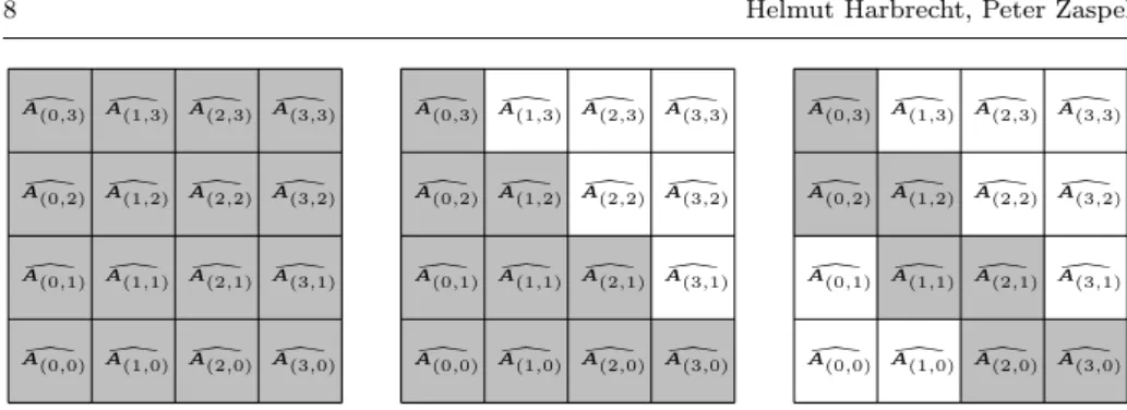
Fig. 1 For discretization levelJ= 3, multilevel frames on the full tensor product space require a very densely populated system matrixdAJ (left), while sparse approximation leads to the system matrixAgJ (center)with smaller size due to fewer active (i.e. gray) matrix subblocks. The sparse grid combination technique(right)leads to the most efficient approximation.
By assuming an underlying d-dimensional finite element discretization with mesh widthh and a multigrid-type linear solver, solving the linear system in (9) would require at leastO
h−2d operations, in contrast toO h−d
for the problem given by (2). This amount of computational work is prohibitively large, especially for larger d. Therefore, we shall find a way to reduce the amount of work to solve this problem. Before we do that, we change the problem discretization to a multilevel discretization, which is the basis for the subsequent sparse approaches.
3.1 Multilevel frames for tensor product constructions
To extend the solution approach from Section 2.2 to tensor product problems, we first recall that we had in theunivariatemultilevel frame case matrix blocks of the form Aj =Aj1j2:=P J j1AJP j2 J ,
withPjJ,PJj as defined in (5) by applying coarsening and the transfer operators of algebraic multigrid. In the univariate case, the multilevel frame linear system of equations was
AJuJ =fJ,
AJ = [Aj]kjk`∞≤J, uJ = [uj]|j|≤J, fJ = [fj]|j|≤J.
By tensorizing this problem, we naturally get the tensor-product frame linear system of equations d AJUJ =FJ, (10) with d AJ = [Aj1j2⊗Aj01j20]k(j1,j10)k`∞,k(j2,j20)k`∞≤J, and UJ = [Uj]kjk`∞≤J, FJ = [Fj]kjk`∞≤J.
For a given right-hand sideFJ, we can construct the corresponding blocksFj by
Fj =Fj1j2:= Pj1 J ⊗P j2 J FJ.
The corresponding vectors and matrices are (usingj = (j1, j2)) of the dimension-alities
Aj⊗Aj0 ∈RNj1Nj10×Nj2Nj02 and Uj,Fj ∈RNj1Nj2.
In order to characterize the computational complexity for the solution of (10), we recall that we assume to have a constant operator complexity for the sequence of matrices Ajj = Aj, i.e. Pη(Aj) ≤ c η(AJ). Moreover, by definition of the Kronecker product, we have the number of non-zeros in each block ofAdJ given by
η(Aj⊗Aj0) =η(Aj)η(Aj0), from which it is easy to verify that we have
η(dAJ) =η(AJ)η(AJ),
with AJ from Section 2.2. It remains to find an upper bound to the number of
non-zeros of the univariate multilevel frame system matrix. Here, we compute
η(AJ) =η [Aj]kjk`∞ ≤J = J X j1=1 J X j2=1 η(Aj1j2)≤ J X j1=1 J X j2=1 η(Amax(j1,j2),max(j1,j2)) =JX j η(Ajj)≤CAJ η(AJ).
In the last equality, we used that we have η(Aj1j2) =η(Aj2j1). The last
inequal-ity corresponds to our assumption on the operator complexinequal-ity. Since we have
J∼O(|logh|), we finally get
η(AdJ)≤c CA2|logh|2η(AJ)2.
This means that the computational work to solve (10) is asymptotically identical to a solve of (9), up to a logarithmic term. Moreover, by using recursive techniques known from the BPX-preconditioner [2], we could even avoid the logarithmic term.
Figure 1 displays the matrix blocks A\(j,j0) := Amax(j
1,j2),max(j01,j20) that are
used by the tensor product multi-level frame system. We limit ourselves to this subset of matrices for the ease of visualization. However, following [16], we in fact only need these matrices to construct AcJ, if appropriate prolongation and restriction operators are considered.
3.2 Sparse tensor product construction
Solving (9) or (10) would be prohibitively expensive, cf. Figure 1. As in the ge-ometric multilevel case, we now assume that the solution of the elliptic problem (1) onΩisHsregular. Therefore, the solution of the tensor product problem (8) becomesHmixs -regular, see [20]. This allows to follow, for example, the lines of [16]
to introduce a sparse, however now algebraically constructed, version of the dis-cretized problem. Instead of using all sub-problems for multi-indices kjk`∞ ≤J, the sparse approximation is reduced to multi-indiceskjk`1≤J. Thereby, we obtain
a new system of linear equations
g
with
g
AJ := [Aj1j2⊗Aj10j02]k(j1,j01)k`1,k(j2,j02)k`1≤J,
g
UJ = [Uj]kjk`1≤J, FgJ = [Fj]kjk`1≤J.
Figure 1 compares both choices in the plots on the left-hand side and the center, recalling that we use only matricesA\(j,j0) :=Amax(j
1,j2),max(j01,j20)in this figure,
see last section. It is easy to see, that this choice should be much more efficient. To show that it is actually more efficient, we now discuss the number of non-zeros inAfJ. Similar to the extimate of the number of non-zeros in the univariate multi-level system matrix, we now compute
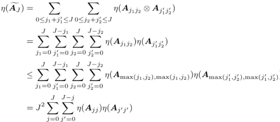
η(AfJ) = X 0≤j1+j01≤J X 0≤j2+j02≤J η(Aj1j2⊗Aj10j02) = J X j1=0 J−j1 X j0 1=0 J X j2=0 J−j2 X j0 2=0 η(Aj1j2)η(Aj10j02) ≤ J X j1=0 J−j1 X j0 1=0 J X j2=0 J−j2 X j0 2=0
η(Amax(j1,j2),max(j1,j2))η(Amax(j10,j20),max(j10,j02))
=J2 J X j=0 J−j X j0=0 η(Ajj)η(Aj0j0)
As discussed before, there is not much theory on the size of the levels in the algebraic multilevel construction. The only available information is the assumed bound on the operator complexity. However, this does not give enough information to finish the above estimate. Nevertheless, the bound on the operator complexity implies a similar scaling of the non-zeros with leveljas in the geometric multilevel construction. Therefore, we here assume to have the same number of non-zeros for each matrix Ajj as in the geometric construction, to give a hint towards the possible performance improvement by the algebraic sparse construction.
With this in mind, we follow the previous example of (linear) finite elements on a mesh with mesh widthh. The number of non-zero entries for matrix Aj is proportional to the number of elements and therefore
η(Ajj) =O(2d j). By extending the above estimate, we get
η(AfJ) =J2 J X j=0 J−j X j0=0 η(Ajj)η(Aj0j0) =c J2 J X j=0 J−j X j0=0 2d j2d j0 =c J2 J X j=0 J X k=j 2d j2d(k−j)=c J2 J X j=0 J X k=j 2d k=O J32d J
Moreover, we haveJ=O(|logh|). That is, the number of non-zeros in the system matrix inAgJ is asymptotically η g AJ =O |logh|3h−d .
That is, in case a BPX-type preconditioner [2, 5, 7, 18] is used, the computational complexity of the problem on the tensor product domainΩ×Ωis (up to a logarith-mic factor) reduced to the computational complexity of the problem on domain
Ω. Moreover, by applying an optimal approach for the construction of the sub-problem matricesAj⊗Aj0 [1, 3, 26], the remaining logarithmic factors might eben be dropped.
3.3 Sparse grid combination technique
It has been shown in [15] that the previous sparse approximation is equivalent to the so-called sparse grid combination technique. The latter one starts approx-imating tensor product problems from a sequence of finite dimensional function spaces
V0(i)⊂V1(i)⊂. . .⊂VJ(i)⊂. . .⊂V(i)
of increasing accuracy, whereiindicates the domain to which the function space is associated. Since we operate onΩ×Ω, we havei= 1,2. As next step, hierarchical increment spacesWj(i) are considered such that
Vj(i):=Wj(i)⊕Vj(−1i) ,
whereW0(i):=V0(i). As usual in sparse (grid) approximation, the (two-dimensional) sparse approximation spaceVcJ is then, cf. [9], defined as
c VJ:= J M j0=0 WJ(1)−j0⊗V (2) j0 = J M j0=0 VJ(1)−j0 V (1) J−1−j0 ⊗Vj(2)0 = J M j0=0 h VJ(1)−j0⊗V (2) j0 VJ(1)−1−j0⊗V (2) j0 i . (11)
The combination technique computes (anisotropic) full-grid solutions on the sub-spaces involved in equation (11) and combines them using appropriate projection. Translated to our problem setting, this approximation is given as
d UJ = J X j0=0 h PJJ−j0⊗PJj0 UJ−j0,j0− PJJ−1−j0⊗PJj0 UJ−1−j0,j0 i = X kjk`1=J (PJj ⊗PJj0)Uj − X kjk`1=J−1 (PJj ⊗PJj0)Uj. (12)
To compute it, we have to solve the decoupled problems
c
AjUj = (Aj1j1⊗Aj2j2)Uj=Fj, wherekjk`1∈ {J, J−1}. (13)
On the right-hand side of Figure 1, the sub-matrices Acj used in this
approx-imation have been marked gray. As before, one can easily verify that the total number of non-zeros of the matrices in (13) is asymptoticallyO
|logh|h−d
for the case of linear finite elements on a tetrahedral mesh with mesh width h in
ddimensions and a geometrically constructed multilevel structure. However, Fig-ure (1) easily clarifies that the pre-asymptotic number of non-zeros in the matrices involved in the combination technique is much smaller than the non-zeros in the sparse approximation discussed before.
In terms of computational complexity of the combination technique, let us re-mind that the (approximate) solution of each sub-problem in (13) can be realized by an iterative linear solver with matrix-vector products. To be more specific, tensor product versions of standard iterative solvers can be constructed, by re-shaping a given iterateUj=(j,j0)∈RNj·N
0
j (and the appropriate right-hand side)
to a matrix of sizeNj×Nj0. Then, the action of one step of an iterative solver for matrixAcj =Aj⊗Aj0 is done by first applying the iterative solver step forAj to all Nj0 columns of the reshaped matrix and by second applying the iterative solver step forAj0 to all Nj rows of the reshaped matrix. One easily verifies that the Kronecker product of two matricesAj,Aj0 withO(Nj),O(Nj0) non-zeros has
O(NjNj0) non-zeros. This leads to a computational complexity ofO(NjNj0) for a single matrix-vector product.
Next, we observe that we actually need only a problem-size independent con-stant number of iterations, if we choose an appropriate solver. Since we have all prolongation and restriction operators from AMG at our disposal, we can actually build a tensor product version of algebraic multigrid. The construction of a tensor-product AMG follows the idea outlined above, i.e. we apply univariate versions of AMG to the columns and rows of a reshaped iterate Uj=(j,j0) of size Nj×Nj0. The tensor-product AMG gives us the property of problem-size independent con-vergence for each sub-problem in (13), i.e. we needO(NjNj0) operations for each sub-problem.
While we have no theory on the number of unknowns on each level of our al-gebraically constructed combination technique, we can still give an analogy from the geometric setting, in order to predict the overall complexity of the method. In case our algebraical construction would behave exactly as a geometrically con-structed multilevel hierarchy, we would have the relationNj =O(2dj). Thereby, the solution of each sub-problem would require O(2d(j+j0)) operations. Since it holdskjk`1∈ {J, J−1}, we can compute
X kjk`1∈{J,J−1} 2d(j+j0)= X kjk`1=J 2d(j+j0)+ X kjk`1=J−1 2d(j+j0) = (J+ 1)2dJ+J2d(J−1).
Hence, we would finally end up with a computational complexity of O(J2dJ) or
O(NJlogNJ).
4 Implementation
In our numerical results, we approximate solutions for tensor product finite element discretizations of elliptic problems based on the combination technique withΩ⊂
R2,3. To this end, we assemble system matrices for a given problem, construct the multilevel hierarchies, solve the decoupled, anisotropic problems in (13) and combine the solutions following the combination rule (12).
Assembly of system matrices. The discretization by the finite element method is done with theMatlab PDE Toolbox ofMatlab 2017a. We use linear finite elements and construct meshes with maximum element size Hmax= 2−J. Furthermore, we use the option Jiggle to optimize the mesh in quality. The stiffness matrix (in-corporating boundary conditions) is constructed by using the Matlab command
assembleFEMatriceswith optionnullspace. In a similar way, we extract the mass
matrix. Afterwards, both matrices and the mesh node coordinates are stored to files.
Construction of the multilevel hierarchy. From within Matlab we call an in-house ad-hoc code that uses the parallel linear solver libraryhypre [6] in version 2.11.1. This library contains the implementation BoomerAMG of classical Ruge-St¨uben AMG. The code reads the stiffness matrix from file and creates the AMG mul-tilevel hierarchy by using hypre. In addition tostandard coarsening with strength measurestr= 0.25 andstandard interpolation, we use two passes ofJacobi interpo-lation with a truncation of the Jacobi interpointerpo-lation with a threshold of 0.001 for the two-dimensional problems and 0.01 for the three-dimensional problem (being treated in Section 5). All other parameters are kept as the defaults ofBoomerAMG. After having created the multigrid hierarchy, the program stores the prolongation matrices of all created levels to files. These are read byMatlab.
Solution of the anisotropic tensor product problems. Based on the prolongation ma-trices and the system matrix AJ on the finest levels, the decoupled problems in (13) can be set up. As discussed before, a tensor product version of AMG is used to solve the systems of linear equations. In our implementation, we construct the sub-problem operators in (13) by individually multiplying the transfer operators between two consecutive levels.
Our tensor product AMG is iterated until the convergence criterion kRitjk`2/kFjk`2≤tol
is fulfilled, whereRitj is the residual of the current iterateUitj in the solver. Since the problems in (13) completely decouple, we can easily parallelize their solution process by aparforloop inMatlab. In case an individual problem becomes very ex-pensive, we further implemented a distributed memory parallelization for the ten-sor product AMG based onMatlab’sdistributedfunction. Thereby, we overcome the limitation of a non-existing multi-core parallelization for sparse matrix-vector products inMatlab.
Combination of the solutions. In the combination phase, we avoid to prolongate the full partial solutions to the finest levelJ. Instead, we randomly choseNevalnodes on the product of the finest meshes onΩ×Ω. On these points, we evaluate the combination formula (12) and compute the empirical error measure
e(Uapprox) =kUapprox−Urefk`2/kUrefk`2,
where Uapprox is the approximated solution andUref is an appropriately evalu-ated reference solution. Note that we do not multiply the tensor product of the prolongation with the solution. Instead, we follow the ideas from Section 3.3 for the construction of the tensor product AMG and apply the prolongations direction-wise. The prolongation for each sub-problem is also parallelized by aparforloop.
3 4 5 6 7 8 10−3 10−2 10−1 levelJ relativ e ` 2 error e ( U exact ) error J4−J
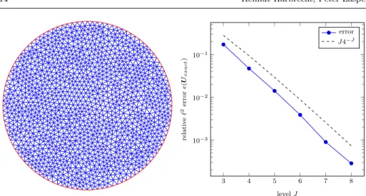
Fig. 2 The combination technique based on our algebraic multilevel hierarchy and applied
to the tensor product of a disk geometry with an unstructured mesh (left, triangulated with
J = 5) shows the same convergence as the geometrically constructed combination technique (right).
5 Numerical results
In our empirical studies, we consider the numerical solution of the problem (∆⊗∆)u=f on Ω×Ω ,
u= 0 on ∂(Ω×Ω). (14)
by means of the combination technique based on the algebraic multilevel hierarchy. Different choices will be made for the domainΩ and the right-hand sidef.
5.1 Analytic example on a disk
The first study is done on a disk domainΩwith center (0,0)> and radius 0.5. We set
f(x,y) = 1.
The exact solution of the resulting problem is
u(x,y) = 1 16 x21+x22−0.52 y12+y22−0.52 .
To approximate the solutionuby the combination technique, we follow the method-ology discussed in Section 4. As part of this, we triangulate the geometry with a maximum element width of 2−J. Figure 2 shows on the left-hand side the resulting mesh for J= 5. It is obvious that the resulting mesh is unstructured. Therefore, classical geometric constructions for the sparse grid combination technique would not be feasible on that mesh. In contrast, our new algebraic approach can solve this problem.
This is shown on the right-hand side of Figure 2, where we compare the nu-merically approximated solution against the above exact solution. Convergence
102 103 104 105 10−3 10−2 10−1 100 101 102 103 104 105
# unknowns (in discretiztion ofΩ)
run tim e of subspace solv es [s] disk (CT) disk (full TP) NJlogNJ NJ2 102 103 104 105 10−3 10−2 10−1 100 101 102 103 104 105
# unknowns (in discretiztion ofΩ)
run time of subspace solv es [s] plate (CT) plate (full TP) NJlogNJ NJ2
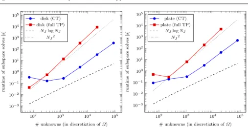
Fig. 3 We compare the runtime of the new combination technique approach (CT) with the
runtime of the traditional the full tensor-product approach (full TP) for the solution of the tensor product elliptic problems on the disk geometry(left)and the plate geometry(right).
# dofs on algebraically coarsened levelj
Ω J\j 0 1 2 3 4 5 6 7 8 9 disk 3 3 11 28 71 4 8 21 52 119 320 5 12 31 84 207 495 1292 6 20 51 139 348 852 2009 5234 7 35 93 244 606 1473 3510 8415 22118 8 46 130 366 978 2469 5983 14480 34081 89097 O(2dj) 1 5 22 87 348 1392 5569 22274 89097 plate 3 5 20 61 4 16 36 90 230 5 28 68 168 414 1072 6 46 116 297 745 1813 4703 7 63 184 515 1272 3117 7491 19611 8 103 302 815 2124 5301 12822 30639 80146 spanner 3 4 10 19 50 117 247 4 11 22 59 147 326 689 1454 5 40 114 300 689 1516 3216 6484 13939 6 210 548 1364 3123 6708 14109 29103 57438 125223 7 1386 3120 6627 14016 29533 61150 124921 253291 496614 1082581
Table 1 For a given problem on levelJ, the algebraic multilevel construction on our example domainsΩconstructs coarser levels with a decrease of the number of unknowns roughly similar to geometric multilevel constructions e.g. in thedisk test case. Above, only those levelsj are reported that are used in the convergence study.
results for the choices J = 3, . . . ,8 are given. From literature, compare e.g. [15], we know that the error of the geometrically constructed sparse grid combination technique scales for the problem under consideration like J4−J. As we can see from the convergence results in Figure 2, the algebraically constructed combina-tion technique shows the same convergence behavior, while being applicable to unstructured grids.
Figure 3 shows on the left-hand side computing times for growing problem size
NJ of the univariate discretization of Ω. We compare the time required for the solution of the combination technique sub-problems with the time required to solve the full tensor-product problem (9) by our tensor-product AMG implementation. Note that we use the coarse grid hierarchies reported in Table 1 for both the
3 4 5 6 7 8 10−3 10−2 10−1 100 levelJ relativ e ` 2 error e ( U appr ox ) error J4−J
Fig. 4 Even for a covariance load on a complex geometry (left, triangulated forJ= 5), the algebraic construction shows the appropriate convergence rate after a short pre-asymptotic phase(right).
combination technique and the full tensor-product approach. All measurements were done on a compute server with dual 20-core Intel Xeon E5-2698 v4 CPU at 2.2 GHz and 768 GB RAM. It becomes evident that our algebraically constructed combination technique approach beats the full tensor-product approach in both, computational complexity and effective runtime. However, both results do not show the predicted computational complexity ofO(NJlogNJ) andO(NJ2). There are several reasons for this behavior.
– First, algebraic multigrid often shows a small, roughly logarithmic, growth in the number of iterations for larger problem sizes, resulting in a slow-down by a logarithmic factor.
– Second, we observe a certain fill-in in the system matrices for coarser problems in the algebraic construction due to our choice of an additional (truncated) Jacobi interpolation. However, this should be pre-asymptotic behavior.
– Third, as can be seen in Table 1, the AMG coarsening approach chosen in our implementation does not show the exact same (asymptotic) decay rateO(2dj) in the number of levels as we expect it from the geometric construction. In fact, this leads to a problem-size dependent growth of the coarsest grid. While this growth does not affect the error decay, it shows up in the computational complexity.
Meanwhile, as stated before, we are able to beat the solution approach based on the full tensor-product approach in terms of computational complexity. Even more, if we would use AMG as solver for the anisotropic sub-problems in thegeometric construction, we would see similar results, anyway. Finally, in terms of runtime, we are by more than two orders of magnitude faster.
5.2 Example on complex geometry with covariance load
The next numerical study is concerned with the solution of the problem (14) with the load f(x,y) = exp −kx−yk2 `
that corresponds to an (unscaled) Gaussian covariance kernel with correlation length `. This is a prototype version of the tensor product elliptic problem on
Ω×Ω showing up in the computation of the output covariance of an elliptic problem onΩwith random input, cf. [16].
In addition to the more complicated right-hand side, we solve the problem for a rather complex geometryΩ. We choose the geomery of a square plate on [0,1]2 with circular wholes of radius 0.15 which are centered at the points
{(0.25,0.25),(0.25,0.75),(0.75,0.25),(0.75,0.75)}.
Figure 4 shows its triangulation forJ= 5 on the left-hand side. Note that it would be almost impossible to solve a problem on such a geometry with the geometrical construction for the sparse grid combination technique. However, with the alge-braic construction, a coarsening to very few degrees of freedom becomes easily possible, compare Table 1.
To be able to compare the above problem against a numerically computed reference solution, we replace the (sampled) covariance kernel for ` = 1 by its low-rank approximation computed with the pivoted Cholesky factorization [14], truncated for a trace norm of 10−8. In this case, depending on the problem size, the truncation results in roughly twenty low-rank terms.
On the right-hand side of Figure 4, we show the convergence results with errors computed against the numerically approximated exact solution by use of the low-rank approximation. After a pre-asymptotic phase, we are able to attain an error that scales likeJ4−J as in the geometric construction.
The problem size dependent runtime to compute the subspace solutions for the plate geometry is given in Figure 3 on the right-hand side. We observe similar compuational complexities and similar runtimes as in the previous example on the disk.
5.3 Large-scale real-world example
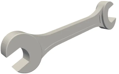
Our last numerical study treats a large-scale problem with a complex real-world geometry Ω. We again aim at solving (14) for f(x,y) = 1. However, we choose thethree-dimensional spanner geometry found in Figure 5. In contrast to the pre-vious examples, we set the maximum mesh width to 25−J, since the geometry is contained in the rather large bounding box [−5,5]×[−12.2,112]×[−15.7,15.7]. Note that the triangulation of Ω results for level J = 7 in a discretization with 1,082,581 unknowns. That is, if we would want to solve the full tensor product problem onΩ×Ω, cf. (8), then we would have to solve a problem with about 1012, that is atrilion, unknowns. This would be clearly out of scope even for large par-allel clusters. In contrast, the combination technique allows to solve this problem. Nevertheless, we still have to solve, e.g. for level J = 7 and the system matrix
\
Fig. 5 In our large-scale real world example, we solve an elliptic problem on the tensor product of the three-dimensional geometry of a spanner. For a discretization level ofJ = 7, the discretization ofΩhas more than a million unknowns. This would lead to 1012, that is a trillion, unknowns in the full tensor product discretization.
3 4 5 6 7 10−1 100 101 102 levelJ relativ e ` 2 error e ( U appr ox ) error J6−J
Fig. 6 Our algebraic multilevel construction for the sparse grid combination technique on the large-scale three-dimensional spanner geometry gradually approaches the optimal convergence rate ofJ2−dJ.
In Figure 6, we show the convergence results for this large scale problem relative to a numerical approximation of the solution. Due to the high dimensionality and complexity of the domainΩ, the convergence results in Figure 6 are only gradually approaching the optimal scaling ofJ2−dJ. Nevertheless, we are able to solve this problem up to a certain accuracy. This shows that even very complex problems of large scale can be solved by the proposed approach.
6 Conclusions
In this work, we have introduced an algebraic construction method for the sparse approximation of tensor product elliptic problems by means of the combination technique. While previous approaches were tight to geometric hierarchies of mesh refinements to build the underlying multilevel discretization, we were able to solve the given type of problems on complex geometries and for unstructured grids by an algebraic multilevel hierarchy based on AMG. We could show that our approach has the same convergence rates as the geometric construction. Measurements of the computational complexity were in the linear range with poly-logarithmic factors. Overall, we are now able to apply sparse approximation for elliptic tensor product problems in a black-box fashion.
References
1. Balder, R., Zenger, C.: The solution of multidimensional real Helmholtz equations on sparse grids. SIAM Journal on Scientific Computing 17(3), 631–646 (1996). DOI 10.1137/S1064827593247035. URL https://doi.org/10.1137/S1064827593247035
2. Bramble, J., Pasciak, J., Xu, J.: Parallel multilevel preconditioners. Mathematics of Com-putation55, 1–22 (1990)
3. Bungartz, H.J.: A multigrid algorithm for higher order finite elements on sparse grids. ETNA. Electronic Transactions on Numerical Analysis 6, 63–77 (1997). URL http://eudml.org/doc/119649
4. Bungartz, H.J., Griebel, M.: Sparse grids. Acta Numerica13, 1–123 (2004)
5. Dahmen, W.: Wavelet and multiscale methods for operator equations. Acta Numerica6, 55–228 (1997)
6. Falgout, R.D., Yang, U.M.: hypre: A library of high performance preconditioners. In: P.M.A. Sloot, A.G. Hoekstra, C.J.K. Tan, J.J. Dongarra (eds.) Computational Science — ICCS 2002, pp. 632–641. Springer Berlin Heidelberg, Berlin, Heidelberg (2002)
7. Griebel, M.: Multilevelmethoden als Iterationsverfahren ¨uber Erzeugendensystemen. Teubner Skripten zur Numerik. B.G. Teubner, Stuttgart (1993)
8. Griebel, M.: Multilevel algorithms considered as iterative methods on semidefinite systems. SIAM International Journal Scientific Statistical Computing15(3), 547–565 (1994) 9. Griebel, M., Harbrecht, H.: On the construction of sparse tensor product spaces.
Mathe-matics of Computation82(282), 975–994 (2013). DOI 10.1090/S0025-5718-2012-02638-X 10. Griebel, M., Harbrecht, H.: On the convergence of the combination technique. In: J. Gar-cke, D. Pfl¨uger (eds.) Sparse grids and Applications – Stuttgart 2014,Lecture Notes in Computational Science and Engineering, vol. 97, pp. 55–74. Springer (2014)
11. Griebel, M., Oswald, P.: Greedy and randomized versions of the multiplicative Schwarz method. Linear Algebra and its Applications7, 1596–1610 (2012)
12. Griebel, M., Schneider, M., Zenger, C.: A combination technique for the solution of sparse grid problems. In: P. de Groen, R. Beauwens (eds.) Iterative Methods in Linear Algebra, pp. 263–281. IMACS, Elsevier, North Holland (1992)
13. Harbrecht, H.: A finite element method for elliptic problems with stochastic in-put data. Applied Numerical Mathematics 60(3), 227–244 (2010). DOI 10.1016/j.apnum.2009.12.002. URL http://dx.doi.org/10.1016/j.apnum.2009.12.002 14. Harbrecht, H., Peters, M., Schneider, R.: On the low-rank approximation by
the pivoted Cholesky decomposition. Applied Numerical Mathematics 62(4), 428–440 (2012). DOI http://dx.doi.org/10.1016/j.apnum.2011.10.001. URL http://www.sciencedirect.com/science/article/pii/S0168927411001814
15. Harbrecht, H., Peters, M., Siebenmorgen, M.: Combination technique based k-th moment analysis of elliptic problems with random diffusion. Journal of Compu-tational Physics 252(C), 128–141 (2013). DOI 10.1016/j.jcp.2013.06.013. URL http://dx.doi.org/10.1016/j.jcp.2013.06.013
16. Harbrecht, H., Schneider, R., Schwab, C.: Multilevel frames for sparse tensor product spaces. Numerische Mathematik110(2), 199–220 (2008). DOI 10.1007/s00211-008-0162-x. URL http://d10.1007/s00211-008-0162-x.doi.org/10.1007/s00211-008-0162-x
17. Hegland, M., Garcke, J., Challis, V.: The combination technique and some generalisations. Linear Algebra and its Applications 420(2), 249–275 (2007). DOI https://doi.org/10.1016/j.laa.2006.07.014. URL http://www.sciencedirect.com/science/article/pii/S002437950600334X
18. Oswald, P.: Multilevel finite element approximation. Theory and applications. Teubner Skripten zur Numerik. B.G. Teubner, Stuttgart (1994)
19. Ruge, J., St¨uben, K.: Algebraic multigrid (AMG). In: S. McCormick (ed.) Multigrid Methods, Frontiers in Applied Mathematics, vol. 5. SIAM, Philadelphia (1986)
20. Schwab, C., Todor, R.A.: Sparse finite elements for elliptic problems with stochastic loading. Numerische Mathematik 95(4), 707–734 (2003). DOI http://dx.doi.org/10.1007/s00211-003-0455-z
21. Schwab, C., Todor, R.A.: Sparse finite elements for stochastic elliptic problems: Higher order moments. Computing71(1), 43–63 (2003). DOI 10.1007/s00607-003-0024-4. URL http://dx.doi.org/10.1007/s00607-003-0024-4
22. St¨uben, K.: A review of algebraic multigrid. Journal of Computational and Applied Math-ematics128(1-2), 281–309 (2001). Numerical Analysis 2000. Vol. VII: Partial Differential Equations
23. Trottenberg, U., Schuller, A.: Multigrid. Academic Press, Inc., Orlando, FL, USA (2001) 24. Yang, U.M.: On long-range interpolation operators for aggressive coarsening. Numerical Linear Algebra with Applications17(2-3), 453–472 (2010). DOI 10.1002/nla.689. URL http://dx.doi.org/10.1002/nla.689
25. Zaspel, P.: Subspace correction methods in algebraic multi-level frames. Linear Algebra and its Applications488, 505–521 (2016). DOI https://doi.org/10.1016/j.laa.2015.09.026. URL http://www.sciencedirect.com/science/article/pii/S0024379515005418
26. Zeiser, A.: Fast matrix-vector multiplication in the sparse-grid Galerkin method. SIAM Journal of Scientific Computing47(3), 328–346 (2011). DOI 10.1007/s10915-010-9438-2. URL https://doi.org/10.1007/s10915-010-9438-2