E-quality control: A support vector machines approach

(1)

Journal of Computational Design and Engineering 3 (2016) 91–101

E-quality control: A support vector machines approach

Tzu-Liang (Bill) Tseng

a

, Kalyan Reddy Aleti

a

, Zhonghua Hu

a

, Yongjin (James) Kwon

b,n

a

Department of Industrial, Manufacturing and Systems Engineering, The University of Texas at El Paso, El Paso, TX 79968, USA

b

Department of Industrial Engineering, Ajou University, Suwon 443–749, South Korea Received 7 January 2015; received in revised form 15 June 2015; accepted 15 June 2015

Available online 9 July 2015

Abstract

The automated part quality inspection poses many challenges to the engineers, especially when the part features to be inspected become complicated. A large quantity of part inspection at a faster rate should be relied upon computerized, automated inspection methods, which requires advanced quality control approaches. In this context, this work uses innovative methods in remote part tracking and quality control with the aid of the modern equipment and application of support vector machine (SVM) learning approach to predict the outcome of the quality control process. The classiﬁer equations are built on the data obtained from the experiments and analyzed with different kernel functions. From the analysis, detailed outcome is presented for six different cases. The results indicate the robustness of support vector classiﬁcation for the experimental data with two output classes.

&2015 Society of CAD/CAM Engineers. Production and hosting by Elsevier. This is an open access article under the CC BY-NC-ND license (http://creativecommons.org/licenses/by-nc-nd/4.0/).

Keywords:Support vector machines; Part classiﬁcations; Remote inspection; Networked robotic station; e-quality

1. Introduction

It is more likely that the rapid advancements in sensor, computer, communication, and information technologies are bringing about the fundamental changes in manufacturing settings. This includes fully-automated, 100% quality

inspec-tion that can process a large amount of measurement data[1–

6]. Other production related activities and business functions

will be also integrated into the company information manage-ment network, which guarantees the instant access to critical

production data for enhanced decision making[7–9]. This new

approach is referred to as e-quality control, and one of the enabling tools is the ability to predict the variations and performance losses during the various production stages. This means that the traditional quality control scheme, which relies on sampling techniques, would be replaced by the sensor-based, automatic, computerized inspection methods that pro-vide the unprecedented level of data processing and handling. Since the production equipment is integrated into the network,

the condition of the machines can be monitored, while the

product quality from speciﬁc machines can be instantly

identiﬁed. In order to test the new quality control approach,

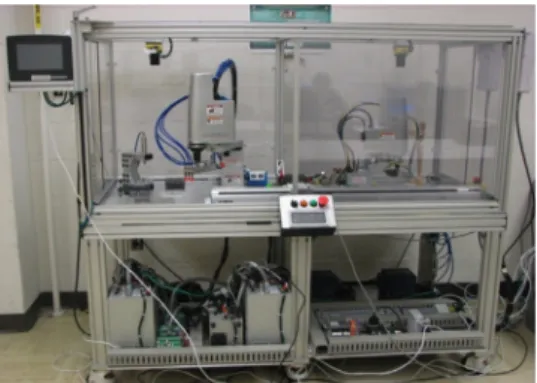
the authors have developed a networked quality control station. This includes two network-accessible assembly robots, two networked vision sensors, and other ancillary equipment which constitutes the cell. The overall setting of the system is

presented inFig. 1.

The vision sensors see the part and measure the dimensions.

The captured image has 640480 pixel size and the analysis

results are produced by the computer algorithms. Part gauging is established by using a pattern matching technique. For each

part, the vision sensor conducts the pre-deﬁned quality control

tasks, and sends the information to the awaiting robot. If the part passes the quality standard, it will be picked up by the robot and dropped into the bin. Otherwise, the bad parts will be carried away by the conveyor belt. The picture of entire setup

is shown inFig. 2.

In the context of e-quality control, the objective of this paper is to apply the machine learning approach in the form of support vector machines (SVMs) to predict the outcome of the

part classiﬁcation. Data obtained from the remote inspection

www.elsevier.com/locate/jcde

http://dx.doi.org/10.1016/j.jcde.2015.06.010

2288-4300/&2015 Society of CAD/CAM Engineers. Production and hosting by Elsevier. This is an open access article under the CC BY-NC-ND license (http://creativecommons.org/licenses/by-nc-nd/4.0/).

n_{Corresponding author.}

(2)

experiments will be analyzed using SVM classiﬁer equations to build a model, which can be used for predictions (i.e., good vs. bad quality). The motivation behind this work is to build

robust classiﬁers, which can sort the incoming parts based on

the vision-sensor generated dimensional data into the

prede-ﬁned groups in an automated way.

2. Literature review

Data mining, which is also referred to as knowledge discovery in databases, means a process of nontrivial extraction of implicit, previously unknown and potentially useful informa-tion (such as knowledge rules, constraints, regularities) from data in databases. In modern manufacturing environments, vast amounts of data are collected into the database management systems and data warehouses from all involved areas, such as product and process design, assembly, materials planning and control, order entry and scheduling, maintenance, recycling, and so on. Different researchers tried to solve the quality control and inspection using various machine learning approaches in an effort to address different types of problems. Automated diagnosis of sewer pipe defects was done using support vector machines (SVMs), where the results showed that the diagnosis accuracy using SVMs was better than that derived by a

Bayesian classiﬁer [10]. A combination of fuzzy logic and

SVMs was used in the form of Fuzzy support vector data

description (F-SVDD) for the automatic target identiﬁcation for

a TFT-LCD array process, where the experimental results indicated that the proposed method ensemble outperformed

the commonly used classiﬁers in terms of target defect

identiﬁcation rate[11]. Independent component analysis (ICA)

and SVMs were used as a combination for intelligent faults diagnosis of induction motors, where the results show that the

SVMs achieved high performance in classiﬁcation using

multi-class strategy, one-against-one and one-against-all [12]. Fault

diagnosis was also done based on the particle swarm optimiza-tion and support vector machines, where the new method can select the best fault features in a short time and has a better real-time capacity than the method based on principal component

analysis(PCA) and SVMs [13]. Multi-class support vector

machines were used for the fault diagnostics of roller bearing using kernel based neighborhood score multi-class support vector machine, where it was shown the multi-class SVM was effective in diagnosing the fault conditions and the results were

comparable with binary SVM [14]. Artiﬁcial neural networks

were used for addressing quality control issue as a non-conventional way to detect surface faults in mechanical front seals, which achieved good results in comparison with the

deterministic system which was already implemented [15].

Fuzzy association rules were used to develop an intelligent quality management approach with the research providing a generic methodology with knowledge discovery and the coop-erative ability for monitoring the process effectively and

efﬁciently [16]. An automatic optical inspection was adopted

for on-line measurement of small components on the eyeglasses assembly line, which was designed to be used at the beginning

of the assembly line and is based on artiﬁcial vision, exploits

two CCD cameras and an anthropomorphic robot to inspect and

manipulate the objects[17].

In fact, the very insightful resources are abounded in terms of fuzzy learning with kernels and SVMs. One example includes the learning of one-class SVM, which requires non-labeled data

[18,19]. Other studies also utilized the method of non-labeled

data, hence being able to operate in a fully unsupervised manner

[20,21]. Fuzzy analytical hierarchy process was used to select

unstable slicing machines to control wafer slicing quality, where the results of exponentially weighted moving average control chart demonstrated the feasibility of the proposed algorithm in effectively selecting the evaluation outcomes and evaluating the

precision of the worst performing machines [22]. Logistic

Regression and PCA were the data mining algorithms used for monitoring PCB assembly quality, where the results demonstrated that the statistical interpretation of solder defect distributions can be enhanced by the intuitive pattern

visualiza-tion for process fault identiﬁcation and variation reduction[23].

Fuzzy logic was used for the fault detection in statistical process control of industrial processes and the comparative rule-based study has shown that the developed fuzzy expert system is

superior to the preceding fuzzy rule-based algorithm [24].

SVMs were used for an intelligent real-time vision system for surface defect detection, where the proposed system was found to be effective in detecting the steel surface defects based on the experimental results generated from over one thousand images

[25]. SVMs were also used as a part of the optical inspection

Internet Yamaha Robot RCX 40 Controller Application Programming Interface Web Cameras

Machine Vision Cameras

Remote Users

Fig. 1. Overall schematic of the proposed e-quality control system.

(3)

system for the solder balls of ball grid array, where the system also gives the training model adjustment judgment core SVM

which is efﬁcient for the image comparison and classiﬁcation

[26]. SVMs were used for quality monitoring in robotized arc

welding, where the results show that the method can be feasible

to identify the defects online in welding production [27]. A

defect classiﬁcation algorithm for the rolling system surface

inspection was developed using Neural Networks and SVMs

with good classiﬁcation ability and generalization performance

[28]. SVMs along with the wavelet feature extraction based on

vector quantization and SVD techniques were used for improved defect detection with the results outlining the impor-tance of judicious selection and processing of 2D DWT wavelet

coefﬁcients for industrial pattern recognition applications as well

as the generalization performance beneﬁts obtained by involving

SVM neural networks instead of other ANN models [29].

Radial basis function (RBF) neural networks (NNS) and SVMs were used for quality monitoring in a plastic injection molding process, where the experimental results obtained thus far

indicate improved generalization with the large margin classiﬁer

as well as better performance enhancing the strength and

efﬁcacy of the chosen model for the practical case study [30].

Two very different studies involve the surface inspection applications, where different approaches can be used within

the similar domains of quality inspection [31,32]. Table 1

summarizes the applications listed in the manuscript.

Although signiﬁcant amount of literature is published on solving

quality related issues using data mining techniques or support vector machines in particular, the concept of addressing e-quality using SVMs remains unexplored. This is due to the fact that the whole

idea of e-quality is still in its developmental stages. However, some researchers developed the idea to address e-quality for manufactur-ing within the framework of internet-based systems. The researchers designed the setup to perform quality control operations over the Internet using Yamaha robots and machine vision cameras. The present work is an extension to this type of work, where the data obtained from these experiments is analyzed using SVMs for predictions. The idea behind using SVMs for this work is solely based on the fact that the performance of SVMs on binary output data is better, when compared to other widely used approaches like the neural networks, principal component analysis and independent component analysis. Most literatures support that SVMs outper-formed better than other methods in many quality applications. Note that the objective of this paper is to focus on determining a better

classiﬁcation model, based on the tuning of the parameters among

different SVM kernels.

3. Methodology

This section explains the model selection for running the

experiments using the support vector classiﬁers, the values of

training parameters selected, and the values of parameters used

for different kernel functions. Fig. 3 shows the conceptual

framework used as a part of this work.

3.1. Model selection

In training SVMs, we need to select a kernel and set a value

to the margin parameter C. To develop the optimal classiﬁer,

Table 1

Support vector machines applications.

Applications Approach Researchers

Automated diagnosis Support vector machines(SVMs) Yang and Su 2008[10]

Automatic target defect identiﬁcation Fuzzy support vector data description (F-SVDD) Liu et al. 2009[11]

Intelligent faults diagnosis Independent component analysis (ICA) and support vector machines (SVMs) Widodo et al. 2007[12]

Fault diagnostics Support vector machine Yuan and Chu 2007[13]

Fault diagnostics Multi-class support vector machine (MSVM) Sugumaran et al. 2008[14]

Surface faults detection Artiﬁcial neural networks Barelli et al. 2008[15]

Intelligent quality management Fuzzy association rules Lau et al. 2009[16]

On-line dimensional measurement Automatic optical inspection Rosati et al. 2009[17]

Optimization Learning with Kernels Schölkopf and Smola 2002[18]

Machine learning One class SVM for classiﬁcation Manevitz and Yousef 2001[19]

Fault detection Residual based fuzzy logic Serdio et al. 2014[20]

Fault detection Multivariate time series modeling Serdio et al. 2014[21]

Quality control Fuzzy analytical hierarchy process Chang et al. 2008[22]

Quality control Logistic Regression, principal component analysis (PCA) Zhang and Luk 2007[23]

Fault detection Fuzzy logic El-Shal and Morris 2000[24]

Surface defect detection Support vector machine Jia et al. 2004[25]

Optical inspection Support vector machine Chen 2007[26]

Quality monitoring Support vector machine Huang and Chen 2006[27]

Surface inspection Neural network, support vector machine Choi et al. 2006[28]

Defect detection Support vector machine Karras 2003[29]

Quality monitoring Radial basis function (RBF) neural networks (NNS), support vector machines (SVMs) Ribeiro 2005[30] Surface inspection SVMs, decision trees with CART and C4.5, fuzzy classiﬁers, K-NN, neural classiﬁers, etc. Eitzinger et al. 2010[31]

(4)

we need to determine the optimal kernel parameter and the

optimal value of C. A k-fold (a value of k¼10) cross

validation approach is adopted for estimating the value of training parameter. The minimum value considered was 0.1 and the maximum value was 500. The value of C with the high

level training accuracy percentage was identiﬁed as the optimal

value (highlighted in bold characters). The performance of the

classiﬁers is evaluated by using different kernel functions in

terms of testing accuracy, training accuracy, a number of support vectors, and validation accuracy. Four different kernel

functions are identiﬁed for this research based on the

knowl-edge gained from the literature review. They include (1) Linear Kernel, (2) Polynomial Kernel, (3) Radial Basis Function (RBF) Kernel, and (4) Sigmoid Kernel. Polynomial and RBF kernels are by far the most commonly used kernels in the

research world. The following section identiﬁes the different

parameters involved in all kernels, and also discusses the range for each parameter.

3.1.1. Linear Kernel

k xi;xj

¼ xi; xj ð1Þ

It is the inner product ofxi; xj, so there is no gamma and

no bias.

3.1.2. Polynomial Kernel

k xi;xj

¼ ðγxixj þcoefficientÞdegree ð2Þ

whereðdegreeAℕ; coefficientZ0; γ40Þ

Two cases are designed based on this kernel, which include

the degrees of 2 and 3. Gamma as 2, coefﬁcient as 1, are

chosen based on the data. Trial and error method was adopted

to ﬁnd the optimal values, which gives high testing data

classiﬁcation accuracy.

3.1.3. Radial Basis Function (RBF) Kernel

k xi;xj ¼exp γjxixjj2 ð3Þ whereðγ 40Þ.

Two cases are also designed based on this kernel with gamma values of 0.5 and 2. Trial and error method was

adopted to ﬁnd the optimal values, which gives high testing

data classiﬁcation accuracy.

3.1.4. Sigmoid Kernel k xi;xj ¼ tan h γxixj þcoefficient ð4Þ whereðγ 40; coefficientZ0Þ.

Values of gamma 0.2 and coefﬁcient 0.1 were chosen for

this work based on the data.

3.2. Training the Support Vector Classiﬁers

After the acquisition of the data from the experiments, the

following characteristics were identiﬁed. Total number of

cases¼138 (note: a total number of times that the experiment

ran. It includes‘auto’and‘manual’modes.). Number of input

features¼5 (note: ﬁve features include the ﬁve different

dimensions of the test piece.). Number of output features¼2

(note: two outputs include the cases where the test piece is

‘compliant’ or ‘non-compliant.). As SVMs are a part of the

supervised learning methods, the data are divided into the training set and testing set. Going with the standard approach, two-thirds of the data are divided into the training set and the remaining one thirds into a testing set. Accordingly, it has been

Remote Inspection Process Data Acquisition Preparing Training Data Model Selection Sensitivity Analysis with different C values Comparing results with different kernels Identifying Optimal Values Different Test Samples Using for future prediction

(5)

set as the training data sample size of 92, and the testing data sample size of 46. According to the literature review, in obtaining the support vectors, one needs to solve the equation:

maximize_α_A_ℝm Wð Þ ¼α Xm i_¼1 αi1=2 Xm i_;j_¼1 αiαjyiyjkðxi;xjÞ ð5Þ subject to the constraints

0rαirCfor alli¼1;…:;m; and

Xm i_¼1

αiyi¼o ð6Þ

Accordingly, one has to estimate the value of the training

parameter C. After closely following the literature and going

through the published materials, it is decided that the k-fold cross validation method is used to estimate the value of

training parameterC.

4. Results and comparisons

In this section, the various steps involved in the process of conducting experiments are presented. The results generated

from using the classiﬁers in six different cases are also shown

in the form of tables. In addition, the comparison between the performances of different kernel functions on the given data is

made and theﬁndings are reported.

4.1. Preparing test samples

The experimental setup considered for this research is in the development stage and as of now it cannot be completely commercialized and used for real-world problems. Due to this reason, a similar scenario is designed, which depicts the real world cases. Instead of parts dealt in a typical production line, small test pieces are designed to conduct the experiment. These pieces are smaller in size, less complicated in dimensions and shapes when compared to the parts used in various types of

industries.Fig. 4shows the geometry of the test piece used in the

experiment, indicating thatL: length of the piece;W: width of the

piece; D1 and D2: diameters of two circles; and CCL: distance

between the circle centers. There are about 20 pieces made. Each differs from the original in at least one dimension, in order to depict that there are defective products in the production line.

4.2. Performing the inspection process

The experiment includes recording real-time measurements on sample work pieces (products) that are passed around on a conveyor belt, compare these dimensions to the required

speci-ﬁcations, make a decision on the quality of the product (i.e. if it is compliant or non-compliant), and take an appropriate action on the product. We used a Cognex DVT 540 vision sensor for making inspections and measurements on the object under test.

We have set the camera to have an image resolution of 640480

bits with an exposure time of 4 ms and a frequency of 2 snapshots per second. The camera is initially trained to learn

the proﬁle of the object being tested and make the required

measurements on it. Once trained, it can detect the presence of the same kind of object under different orientations. The camera can be addressed using an IP address and is capable of exchanging information with other entities over a data network. Subsequently, during inspections, the camera makes measurements on the objects passing on the conveyor belt and reports it back along with the objects' position to an application server over the network. The application is software written in VB6 and runs in a PC. It communicates with the camera over the network and receives the measurement and position information about the object. It then uses this information to decide whether the product

adheres to the required speciﬁcations. Once a decision is made, it

communicates with the robot over the network, and instructs it to it stop the belt and do the proper pick and place operation on the object. The robot places the compliant and non-compliant objects on to two different stacks. The camera placed at the inspection site also allows for visual monitoring of the ongoing process from

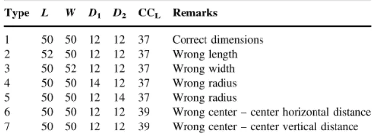
a remote location.Table 2summarizes the speciﬁcations for the

different type of work pieces used for the experiment. Type 1

constitutes objects that adhere to the required speciﬁcations. The

other types deviate from these speciﬁcations in one dimension.

4.3. Data acquisition

Based on the previous phase, the experiment is conducted allowing the user to test the different samples. The user has CCL

W

D1

D2

L

Fig. 4. Test Piece Geometry.

Table 2

Work piece speciﬁcations (units: mm). Type L W D1 D2 CCL Remarks 1 50 50 12 12 37 Correct dimensions 2 52 50 12 12 37 Wrong length 3 50 52 12 12 37 Wrong width 4 50 50 14 12 37 Wrong radius 5 50 50 12 14 37 Wrong radius

6 50 50 12 12 39 Wrong center–center horizontal distance 7 50 50 12 12 39 Wrong center–center vertical distance

(6)

two options to perform this type of experiment, which includes dealing with the robot in manual and auto modes. The data used for this experiment consists of data recorded in two modes. (1) Manual mode: after the test piece is placed on the conveyor system, it stops as soon as it comes right below the DVT vision sensor, which records the dimensions. Through a VB interface, the user is able to see the values and has to make a judgment whether the test piece is compliant or non-compliant. After the user takes a decision the robot is programmed to pick up the object and place it in the respective stack. The process continues until all test samples are put on

the conveyor. The signiﬁcance of this mode lies on the users'

ability to make the correct decision to classify the object. (2) Auto mode: the process is almost similar to the manual mode except after the dimensions are recorded by the DVT vision sensor camera, the application itself takes the decision, whether the piece is compliant or non-compliant. The VB application has the option to write all the data recorded along

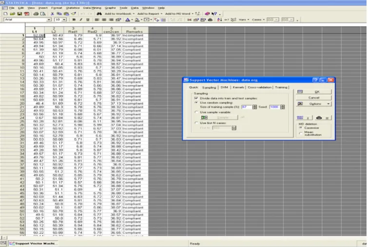
with the action taken into an excelﬁle. Most analysis part is

done using a statistics software package, called STATISTICA, which provides a selection of data analysis, data management,

data mining, and data visualization procedures. Fig. 5shows

the screen shot of the input data used for the analysis in the STATISTICA 8.0 data mining module.

4.4. Case studies

Results obtained from six different cases are presented in this section. All cases vary in the type of kernel functions used

for classiﬁcation. The cases include: Case 1. Radial Basis

Function Kernel (gamma¼0.5); Case 2. Radial Basis Function

Kernel (gamma¼2.0); Case 3. Polynomial Kernel (degree¼2,

gamma¼2, coefﬁcient¼1); Case 4. Polynomial Kernel

(degree¼3, gamma¼2, coefﬁcient¼1); Case 5. Linear

Ker-nel; and Case 6. Sigmoid Kernel (gamma¼0.2,

coefﬁcient¼0.1).

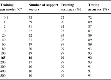
4.4.1. Case 1. Radial Basis Function Kernel (gamma¼0.5)

The classiﬁer equations are tested with the radial basis

function kernel using a gamma value of 0.5 and different runs are made using different values of the training parameter. For each run, a number of support vectors generated, while the accuracy of classifying the data in the training and testing sets

are noted. The summary is presented inTable 3.

Values from the table are plotted in the form of a graph

shown inFig. 6with training parameter values on theX-axis

and accuracy percentages on theY-axis. Optimal cross

valida-tion value is found and highlighted in the graph. Fig. 5. Screen shot of the STATISTICA 8.0 interface.

(7)

4.4.2. Case 2. Radial Basis Function Kernel (gamma¼2.0)

The classiﬁer equations are tested with the radial basis

function kernel using a gamma value of 2 and different runs are made using different values of the training parameter. For each run, a number of support vectors generated the accuracy of classifying the data in the training and testing sets are noted.

The summary is presented inTable 4.

The values from the table are plotted in the form of a graph

shown inFig. 7using Statistica with training parameter values

on theX-axis and accuracy percentages on theY-axis. Optimal

cross validation value is found and highlighted in the graph.

4.4.3. Case 3. Polynomial Kernel (degree¼2, gamma¼2,

coefﬁcient¼1)

The classiﬁer equations are tested with the polynomial

kernel and different runs are made using different values of the training parameter. For each run, a number of support vectors are generated, and the accuracy of classifying the data

in the training and testing sets are noted. The summary of all

these observations is presented in Table 5.

on the X-axis and the accuracy percentages on the Y-axis.

Optimal cross validation value is found and highlighted in the graph.

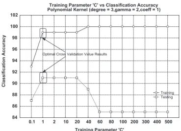
4.4.4. Case 4. Polynomial Kernel (degree¼3, gamma¼2,

coefﬁcient¼1)

The classiﬁer equations are tested with the Polynomial

Kernel and different runs are made using different values of the training parameter. For each run, a number of support vectors generated, and the accuracy of classifying the data in the training set and testing set are noted. The summary of all

these observations is presented in Table 6.

on the X-axis and the accuracy percentages on the Y-axis.

Table 3

Summary table for Case 1. Training parameter‘C’ Number of support vectors Training accuracy (%) Testing accuracy (%) 0.1 72 72 72 1 39 90 89 2 31 92 87 10 22 93 87 20 22 93 89 40 21 98 89 60 19 99 89 80 20 99 93 100 19 99 93 165 16 99 93 200 17 99 93 300 10 99 91 400 10 99 91 500 10 99 91

Training Parameter 'C' vs Classification Accuracy RBF Kernel (gamma = 0.5) 0.1 1 2 10 20 40 60 80 100 165 200 300 400 500 Training Parameter 'C' 70 75 80 85 90 95 100 105 C la s sific a ti o n Ac cu ra cy Training Testing Optimal Cross Validation Value Results

Fig. 6. Graph showing different‘C’values plotted against accuracy levels.

Table 4

Training Parameter 'C' vs Classification Accuracy RBF Kernel (gamma = 2.0) 0.1 1 2 10 20 40 60 80 100 200 300 376 400 500 Training Parameter 'C' 86 88 90 92 94 96 98 100 C la s sific a tion Ac c u racy Training Testing Optimal Cross Validation Value Results

(8)

Optimal cross validation value is found and highlighted in the graph.

4.4.5. Case 5. Linear Kernel

The classiﬁer equations are tested with Linear Kernel and

different runs are made using different values of the training parameter. For each run, a number of support vectors are generated, and the accuracy of classifying the data in the training set and testing set are noted. The summary of all these

observations are presented inTable 7.

shown inFig. 10. Optimal cross validation value is found and

highlighted in the graph.

4.4.6. Case 6. Sigmoid Kernel (gamma¼0.2, coefﬁcient¼0.1)

The classiﬁer equations are tested with the Sigmoid Kernel

and different runs are made using different values of the training parameter. For each run, a number of support vectors are generated, and the accuracy of classifying the data in the training set and testing set are noted. The summary is

presented inTable 8.

shown inFig. 11. Optimal cross validation value is found and

highlighted in the graph. Table 5

Training Parameter 'C' vs Classification Accuracy Polynomial Kernel (degree =2,gamma = 2,coeff = 1)

0.1 1 2 6 10 20 40 60 80 100 200 300 400 500 Training Parameter 'C' 84 86 88 90 92 94 96 98 100 102 C la s sification A c cur acy Training Testing Optimal Cross Validation Value Results

Table 6

Summary table for Case 4. Training parameter‘C’ Number of support vectors Training accuracy (%) Testing accuracy (%) 0.1 20 93 87 1 13 99 91 2 12 99 91 10 8 99 91 20 9 99 91 40 8 100 89 60 8 100 85 80 8 100 85 100 8 100 85 200 8 100 85 300 8 100 85 400 8 100 85 500 8 100 85

Training Parameter 'C' vs Classification Accuracy Polynomial Kernel (degree = 3,gamma = 2,coeff = 1)

0.1 1 2 10 20 40 60 80 100 200 300 400 500 Training Parameter 'C' 84 86 88 90 92 94 96 98 100 102 Classification Accuracy Training Testing Optimal Cross Validation Value Results

Table 7

(9)

4.5. Comparison

This section compares the results obtained from the different cases. After executing the model with different kernel

func-tions, the results that a speciﬁc kernel gives the best accuracy

are identiﬁed and used for comparison along with other

kernels.Table 9 summarizes theﬁnding.

Additionally, to show the advantage of the SVMs, two other methods that are commonly used have been tested. The results

are shown inTable 10.

5. Conclusions

This section presents the importantﬁndings that can be drawn

from the analyses. The purpose of this research was to develop a

support vector classiﬁer model based on the experimental data

in order to facilitate the process of e-quality control. The study was conducted under the following assumptions. (1) The data used for analysis contained 138 different cases, which were obtained by running the experiment with different test samples.

(2) The model selection for training parameterCwas based on

the v-fold cross validation approach. (3) The range of training

parameter C values included 0.01 to 500, where much higher

values in the order of four digits andﬁve digits can also be used

based on the characteristics of data. (4) The parameters of the kernel functions were assumed based on the trial and error, to obtain the best accuracy level. After analyzing the data obtained

Training Parameter 'C' vs Classification Accuracy Linear Kernel 0.1 1 2 10 20 40 60 80 100 200 300 400 476 500 Training Parameter 'C' 74 76 78 80 82 84 86 88 90 92 94 96 98 Classification Accuracy Training Testing Optimal Cross Validation Value Results

Table 8

Training Parameter 'C' vs Classification Accuracy Sigmoid Kernel (gamma = 0.2, coeff = 0.1)

0.1 1 2 10 16 20 40 60 80 100 200 300 400 500 Training Parameter 'C' 55 60 65 70 75 80 85 90 95 Classification Accuracy Training Testing Optimal Cross Validation Value Results

Table 9 Summary of experiments. Kernel Training parameter‘C’ Train rate (%) Test rate (%) SVs Linear 476 97 93 18(7a) Polynomial (degree ¼2) 6 99 93 14(8a) Polynomial (degree ¼3) 1 99 91 13(6a₎ RBF (gamma¼0.5) 165 99 93 16(6a₎ RBF (gamma¼2) 376 99 93 13(1a₎ Sigmoid (gamma¼0.2, coef¼0.1) 16 93 85 30(25a₎ a

Bounded support vectors.

Table 10

Comparison between decision tree and logistics regression methods. Methods Train rate (%) Test rate (%)

Decision tree 97 87

(10)

using SVM classiﬁers and testing the accuracy levels using different kernels, the following conclusions can be drawn. Since

the SVMs produced good classiﬁcation results for data with

binary outcome, the results achieved for this data were

signiﬁcant. The highest testing rate of 93% was achieved, when

using Linear, Polynomial and RBF kernels in different cases. Polynomial kernel of second degree and RBF kernel with gamma values had slightly higher training rate values. Among

all cases, the RBF kernel with a gamma value of 2 is identiﬁed

as the best performer, as it has the lowest number of support

vectors used in the classiﬁcation method. Heuristically, a less

number of support vectors signiﬁes the robustness of the

classiﬁer. However, this might not be true in all cases, since it

also depends on the number of bounded support vectors, which are located between the margins. The value of the training

parameter‘C’identiﬁed as 376 for the RBF kernel also satisﬁes

the basic necessity for selecting the ideal training parameter. If

‘C’is too small, the insufﬁcient stress will be placed onﬁtting

the training data. If it is too large, the algorithm leads to over

ﬁtting the data. As to the data size, even though the available

data are not large, it is adequate for the research. It may have a better result (i.e., a better predict accuracy) with the larger data sets. Basically, there are also problems in dealing with the big

data, such as overﬁtting and outliers. Moreover, the proposed

model may be insensitive only given by certain data sets. In

other words, different data sets may lead various “optimal”

models. Consequently, it is suggested that pre-processing effort could focus on eliminating bias, particularly pre-existing pattern

data prior the use of SVM classiﬁcation. One of the future

works could dedicate to develop a better model, which may be hybrid in nature through combining different approaches (i.e., SVM and non-SVM) and/or fusing different kernel functions under feasible conditions. Another future work might be to realize the equality in the dynamic environments. The new algorithm will be affected by the dynamic data, when setting the parameters automatically to optimize the models.

Acknowledgments

This work was partially supported by the National Science Foundation, United States (Award DUE-1246050) and the US

Department of Education (Award P031S120131 and

P120A130061). This research was also supported by the Basic Science Research Program through the National Research Foundation of Korea (NRF) funded by the Ministry of Education (Grant no. NRF-2013R1A1A2006108). The authors

wish to express sincere gratitude for their ﬁnancial support

received the duration of the research.

References

[1] A. Cohen, Simulation Based Design, DARPA Plus-Up Workshop on SBD Alpha Release (DARPA/TTO Program), 1997.

[2] Bennis F, Castagliola P, Pino L. Statistical analysis of geometrical tolerances. A case study.J. Qual. Eng.2005;17(3)419–27.

[3] Goldin D, Venneri S, Noor A. Newfrontiers in engineering.Mech. Eng. 1998;120(2)63–9.

[4]Goldin D, Venneri S, Noor A. Ready for the future?Mech Eng.1999;121 (11)61–70.

[5]Kwon Y, Wu T, Ochoa J. SMWA. A CAD-based decision support system for the efﬁcient design of welding,.J. Concurr. Eng. Res. Appl. 2004;12(4)295–304.

[6] Y. Kwon, G. Fischer, Three-year vision plan for undergraduate instruc-tional laboratories. Simulation-based, reconﬁgurable integrated lean manufacturing systems to improve learning effectiveness, (A funded proposal with $100,000), College of Engineering Equipment Fund. University of Iowa, Iowa City, 2003.

[7]Waurzyniak P. Moving toward the e-factory. Manufacturing industry takes ﬁrst steps toward implementing collaborative e-manufacturing systems.SME Manuf. Eng.2001;127(5)43–60.

[8]Aronson R. More automation, less manpower. Smarter cells and centers. SME Manuf. Eng.2005;134(6)85–108.

[9] Center for Intelligent Maintenance Systems, 2005, Available at:〈http// wumrc.engin.umich.edu/ims/?page=home〉.

[10]Yang M, Su T. Automated diagnosis of sewer pipe defects based on machine learning approaches,.Expert Syst. Appl.2008;35(3)1327–37. [11]Liu Y, Lin S, Hsueh Y, Lee M. Automatic target defect identiﬁcation for

TFT-LCD array process inspection using kernel FCM-based fuzzy SVDD ensemble.Expert Syst. Appl.2009;36(2)1978–98.

[12]Widodo A, Yang B, Han T. Combination of independent component analysis and support vector machines for intelligent faults diagnosis of induction motors.Expert Syst. Appl.2007;32:299–312.

[13]Yuan S, Chu F. Fault diagnostics based on particle swarm optimization and support vector machines. Mech. Syst. Signal Process. 2007;21: 1787–98.

[14]Sugumaran V, Sabareesh G, Ramachandran K. Fault diagnostics of roller bearing using kernel based neighborhood score multi-class support vector machine.Expert Syst. Appl.2008;34(4)3090–8.

[15]Barelli L, Bidini G, Mariani F, Svanziroli M. A non-conventional quality control system to detect surface faults in mechanical front seals.Eng. Appl. Artif. Intell.2008;21(7)1065–72.

[16]Lau H, Ho G, Chu K, Ho W, Lee C. Development of an intelligent quality management system using fuzzy association rules,.Expert Syst. Appl.2009;36(2)1801–15.

[17]Rosati G, Boschetti G, Biondi A, Rossi A. On-line dimensional measurement of small components on the eyeglasses assembly line. Opt. Lasers Eng.2009;47(3–4)320–8.

[18]Schölkopf B, Smola AJ. Learning with Kernels-Support Vector Machines, Regularization, Optimization and Beyond. London, England: MIT Press; 2002.

[19]Manevitz L, Yousef M. One-class SVMs for document classiﬁcation,.J. Mach. Learn. Res.2001;2:139–54.

[20]Serdio F, Lughofer E, Pichler K, Buchegger T, Efendic H. Residual-based fault detection using soft computing techniques for condition monitoring at rolling mills.Inf. Sci.2014;259:304–20.

[21]Serdio F, Lughofer E, Pichler K, Pichler M, Buchegger T, Efendic H. Fault detection in multi-sensor networks based on multivariate time-series models and orthogonal transformations.Inf. Fusion2014;20:272–91. [22]Chang C, Wu C, Chen H. Using expert technology to select unstable

slicing machine to control wafer slicing quality via fuzzy AHP.Expert Syst. Appl.2008;34:2210–20.

[23]Zhang F, Luk T. A data mining algorithm for monitoring PCB assembly quality.IEEE Trans. Electron. Packag. Manuf.2007;30(4)299–305. [24]El-Shal S, Morris A. A fuzzy expert system for fault detection in

statistical process control of industrial processes.IEEE Trans. Syst. Man Cybern. C. Appl. Rev.2000;30(2)281–9.

[25] H. Jia, Y. Murphey, J. Shi, and T. Chang, An intelligent real-time vision system for surface defect detection, in: Proceedings of the 17th Interna-tional Conference on Pattern Recognition, ICPR’04, vol. 3, 2004, pp. 239–242.

[26] S. Chen, An optical inspection system for the solder balls of BGA using support vector machine classiﬁcation, in: Proceedings of the Sixth International Conference on Machine Learning and Cybernetics, Hong Kong, pp. 19–22, 2007.

(11)

[27]Huang X, Chen S. SVM-based fuzzy modeling for the arc welding process.Mater. Sci. Eng.: A2006;427(1–2)181–7.

[28] K. Choi, K. Koo, and J. Lee, Development of defect classiﬁcation algorithm for POSCO rolling strip surface inspection system, in: Proceedings of the SICE-ICASE International Joint Conference 2006 Oct. 18–21, 2006, Bexco, Busan, Korea.

[29] D. Karras, Improved defect detection using support vector machines and wavelet feature extraction based on vector quantization and SVD techniques, in: Proceedings of the International Joint Conference on Neural Networks, vol. 3, 2003, pp. 2322–2327.

[30] Ribeiro B. Support vector machines for quality monitoring in a plastic injection molding process.IEEE Trans. Syst. Man Cybern. C: Appl. Rev. 2005;35(3)401–10.

[31] Eitzinger C, Heidl W, Lughofer E, Raiser S, Smith J, Ahir M, Sannen D, van Brussel H. Assessment of the inﬂuence of adaptive components in trainable surface inspection systems.Mach. Vis. Appl.2010;21(5)613–26. [32] Heidl W, Thumfart S, Lughofer E, Eitzinger C, Klement E. Machine learning based analysis of gender differences in visual inspection decision making.Inf. Sci.2013;224:62–76.