Variable Selection and Prediction in Messy'' High-Dimensional Data"

(1)

Variable Selection and Prediction in “Messy”

High-Dimensional Data

A THESIS

SUBMITTED TO THE FACULTY OF THE GRADUATE SCHOOL OF THE UNIVERSITY OF MINNESOTA

BY

Benjamin Timothy Brown

IN PARTIAL FULFILLMENT OF THE REQUIREMENTS FOR THE DEGREE OF

Doctor of Philosophy

Julian Wolfson

(2)

c

Benjamin Timothy Brown 2017

(3)

Acknowledgements

There are many people that have earned my gratitude for their contribution to my time in graduate school. My advisor Julian Wolfson helped get me here when I thought I might not make it. Sally Olander had the answer to every question I had along the way. Brad Carlin kept me on track and provided a great deal of needed support.

(4)

Dedication

To my wife, Lindsey, for encouraging me for the past three and a half years and sup-porting me through the many long nights of research.

(5)

Abstract

When dealing with high-dimensional data, performing variable selection in a regression model reduces statistical noise and simplifies interpretation. There are many ways to perform variable selection when standard regression assumptions are met, but few that work well when one or more assumptions is violated. In this thesis, we propose three variable selection methods that outperform existing methods in such “messy data” situ-ations where standard regression assumptions are violated. First, we introduce Thresh-olded EEBoost (ThrEEBoost), an iterative algorithm which applies a gradient boosting type algorithm to estimating equations. Extending its progenitor, EEBoost (Wolfson, 2011), ThrEEBoost allows multiple coefficients to be updated at each iteration. The number of coefficients updated is controlled by a threshold parameter on the magni-tude of the estimating equation. By allowing more coefficients to be updated at each iteration, ThrEEBoost can explore a greater diversity of variable selection “paths” (i.e., sequences of coefficient vectors) through the model space, possibly finding models with smaller prediction error than any of those on the path defined by EEBoost. In a simula-tion of data with correlated outcomes, ThrEEBoost reduced predicsimula-tion error compared to more naive methods and the less flexible EEBoost. We also applied our method to the Box Lunch Study where we found that we were able to reduce our error in predicting BMI from longitudinal data. Next, we propose a novel method, MEBoost, for variable selection and prediction when covariates are measured with error. To do this, we incor-porate a measurement error corrected score function due to Nakamura (1990) into the ThrEEBoost framework. In both simulated and real data, MEBoost outperformed the CoCoLasso (Datta and Zou, 2017), a recently proposed penalization-based approach to variable selection in the presence of measurement error, and the (non-measurement

(6)

tions may be simultaneously violated. Motivated by the idea of stacking, specifically the SuperLearner technique (Van Der Laan et al., 2007), we propose a novel method, Super Learner Estimating Equation Boosting (SuperBoost). SuperBoost performs vari-able selection in the presence of multiple data challenges by combining the results from variable selection procedures which are each tailored to address a different regression as-sumption violation. The ThrEEBoost framework is a natural fit for this approach, since the component “learners” (i.e., violation-specific variable selection techniques) are fairly straightforward to construct and implement by using various estimating equations. We illustrate the application of SuperBoost on simulated data with both correlated out-comes and covariate measurement error, and show that it performs as well or better than methods which address only one (or neither) of these factors.

(7)

List of Tables

2.1 Mean minimum prediction error (a), median variable selection (b)

sensi-tivity and (c) specificity, (d) mean number of iterations (25th and 75th percentile) to attain minimum prediction error, (e) minimum mean QIC, and (f) proportion of simulations where algorithm did not find a unique minimum MSE for ThrEEBoost in the sparse true model under

differ-ent values of the threshold, τ and correlation between intra-individual

observations, ρ. Results are based on 1000 simulations, each with 500

iterations. . . 16

2.2 Mean minimum prediction error (a), median variable selection (b)

sensi-tivity and (c) specificity, (d) mean number of iterations (25th and 75th percentile) to attain minimum prediction error, (e) minimum mean QIC, and (f) proportion of simulations where algorithm did not find a unique minimum MSE for ThrEEBoost in the less sparse true model under

dif-ferent values of the threshold,τ, and correlation between intra-individual

observations, ρ. Results are based on 1000 simulations, each with 1500

ThrEEBoost iterations. . . 19

2.3 Coefficients for the optimal ThrEEBoost (τ = 0.4) and LASSO models

selected by cross-validated MSE. Small coefficients (magnitude < 0.05)

are omitted. “–” indicates that the variable was not selected in the model. 22

(11)

models. (CV MSE) denotes models selected by minimizing cross-validated

MSE. . . 23

3.1 Performance metrics for the 1,000 simulations in various measurement error scenarios. The models were selected at the point with minimum MSE-M. . . 50

3.2 Coefficients, Deviance, and MSE-M from selected models for MEBoost with specified value ofτ and ˆδ2_Dand the Lasso. Small coefficients (magni-tude<0.05) are omitted. “-” indicates that the variable was not selected in the model. . . 51

4.1 List of parameter values for each scenario. nis the number of clusters,σ2 is the residual variance,δ is the standard deviation of the measurement error,ρ is the pairwise correlation in outcomes within clusters,βm is the effect size of mismeasured predictors, βg is the effect size of predictors measured without error. Scenariobin each setting has fewer clusters and higher residual variance, giving us less information to reach an accurate estimate. . . 65

4.2 Performance metrics for scenario 1a. . . 67

4.3 Performance metrics for scenario 1b. . . 68

(12)

List of Figures

2.1 AverageL1distances from the trueβ(top row), estimated coefficient

val-ues (middle row) and MSPE (bottow row) across iterations for various

values of τ, when data are generated from a very sparse true regression

model with an intra-individual correlation ofρ= 0.3. The solid, dashed,

and dotted lines in the coefficient plots (middle row) represent coefficients with true values of 0.5, 0.2, and 0.0 respectively. Results are based on 1000 simulations, each with 500 ThrEEBoost iterations. The solid ver-tical lines show the iteration where the minimum mean squared error is

achieved in each scenario. . . 15

2.2 The distribution of selectedτ values via cross-validation. For each value

ofρ, the medianτCV selected was 0.58. . . 17

(13)

1

ues (middle row) and MSPE (bottow row) across iterations for various

values of τ, when data are generated from a less sparse true regression

model with an intra-individual correlation ofρ= 0.3. The solid, dashed,

and dotted lines in the coefficient plots (middle row) represent coefficients with true values of 0.5, 0.2, and 0.0 respectively. Results are based on 1000 simulations, each with 1500 ThrEEBoost iterations. The solid ver-tical lines show the iteration where the minimum mean squared error is

achieved in each scenario. . . 20

2.4 The distribution of selectedτ values via cross-validation. For each value

ofρ, the medianτCV selected were 0.38, 0.40, and 0.38. . . 21

2.5 Average QIC when data are generated from a less sparse true regression

model with an intra-individual correlation of ρ= 0.3. Results are based

on 1000 simulations, each with 1500 ThrEEBoost iterations. . . 21

2.6 Coefficient magnitudes for the optimal models (chosen by cross-validated

MSE) for different values ofτ. Each row corresponds to a different

vari-able; darker shades of gray correspond to higher coefficient magnitudes. The names of the variables are displayed on the right; a data dictionary giving the variable descriptions is provided in the Supplementary Materials. 25

3.1 Summary statistics for the scenario with varying levels of independent

measurement errors. Plots are of MSE, MSE-M, L1 distance from ˆβ to

the true value ofβ, sensitivity, and specificity across the mean path over

1,000 simulations. . . 48

(14)

ducted comparing the variable selection path of MEBoost to CoCoLasso. Plots are of the number of nonzero coefficients included in the model, the portion of coefficients that are ’mismatched’ with only one of the two models selecting a certain variable, and the element-wise distance in a

coefficient between the two methods. . . 49

4.1 Model weights and traceplots for mean paths of Super Learner models in

scenario 1b. . . 74

4.2 Performance metrics over the paths created by MEBoost in scenario 3a. 75

(15)

Chapter 1

Introduction

Driven by the ever-increasing amount of high-dimensional data in biomedicine, much recent research has focused on how to do variable selection and prediction in problems

where the number of predictors,p, is large in comparison to the number of observations,

n. Traditional approaches like forward selection and backward elimination are widely

employed but have limitations, particularly when the number of covariates is very large. For instance, it has been shown that the first variable selected in forward selection can-didate models can often be the first removed in backwards elimination (Hocking, 1976). Methods such as the Lasso (Tibshirani, 1996) and SCAD (Fan and Li, 2001) generally offer superior variable selection and predictive performance to stepwise techniques, but have been applied almost exclusively to general linear (Park et al., 2006) and survival regression models (Fan and Li, 2002).

Some authors have extended penalized approaches to more complex modeling sit-uations such as correlated outcomes (Johnson et al., 2008), missing covariates (Yang et al., 2005), and measurement error in covariates (Datta and Zou, 2017). However, the resulting statistical procedures often involve constrained optimization of nonconvex functions, and may therefore be too computationally intensive to apply in settings where

pis on the order of hundreds or thousands. Ueki (2009) proposes a smooth thresholding

(16)

approach to penalizing estimating equations, with the selection threshold determined by an adaptive lasso type estimator. While smooth thresholding avoids convex opti-mization and therefore offers a computational speedup, the method still requires that a set of estimating equations be solved numerically for a large number of points on a two-dimensional grid of tuning parameters. Further, since the thresholding relies on an initial “full model” estimator, it is unclear how this technique generalizes to problems

where pis large in relation to n.

As an alternative to penalization methods, Wolfson (2011) introduced EEBoost, a gradient descent-based method that can be used to perform variable selection for any regression problem where estimation of low-dimensional coefficients can be performed by solving an estimating equation. EEBoost iteratively constructs a set of models de-fined by coefficients using a modified steepest descent algorithm wherein the gradient of the loss function is replaced by the relevant estimating equation. The generic EEBoost algorithm is easily implemented using existing statistical software and can be applied to a wide variety of problems. For example, Wolfson (2011) applied EEBoost to gener-alized estimating equations (GEE) for correlated data, and inverse probability weighted estimating equations methods for time-to-event data with missing covariates, and Janes et al. (2012) applied it to doubly robust semiparametric efficient estimating equations for continuous outcome data.

We propose a novel method, Thresholded EEBoost (ThrEEBoost), an extension to EEBoost wherein multiple coefficients may be updated at each iteration; the number of coefficients updated is controlled by a threshold parameter on the magnitude of the estimating equation. By allowing more coefficients to be updated at each iteration, ThrEEBoost can explore a greater diversity of variable selection “paths” (i.e., sequences of coefficient vectors) through the model space, possibly finding models with smaller prediction error than any of those on the path defined by EEBoost. To evaluate our

(17)

method, we will conduct a simulation with a GEE model, we will apply the method to the longitudinal data set of the Box Lunch study.

Next, we will propose an extension of our method to perform variable selection and prediction when covariates are measured with error. To do this, we utilize ThrEEBoost along with a correct score function for covariates with measurement error from Naka-mura (1990). In this section, we will define the new method of Measurement Error Boost (MEBoost) and conduct a simulation study to compare it to the existing method of the CoCoLasso (Datta and Zou, 2017) which we will also describe.

Lastly, we consider that a single data set may encounter more than one data chal-lenge. There has not been much research allocated to dealing with multiple regression assumptions being violated within one data set in either the low or high-dimensional case. We provide a general method to perform variable selection in the presence of multiple data challenges where we combine the machine learning principles of boosting and stacking, specifically the method Super Learner (Van Der Laan et al., 2007). We present a novel method, Super Learner Estimating Equation Boosting (SuperBoost) and examine it’s performance through data simulated with correlated outcomes and covariate measurement error.

(18)

Chapter 2

ThrEEBoost

2.1

Introduction

Driven by the ever-increasing amount of high-dimensional data in biomedicine, much recent research has focused on how to do variable selection and prediction in problems

where the number of predictors,p, is large in comparison to the number of observations,

n. Traditional approaches like forward selection and backward elimination are widely

employed but have limitations, particularly when the number of covariates is very large. For instance, it has been shown that the first variable selected in forward selection can-didate models can often be the first removed in backwards elimination (Hocking, 1976). Methods such as the LASSO (Tibshirani, 1996) and SCAD (Fan and Li, 2001) generally offer superior variable selection and predictive performance to stepwise techniques, but have been applied almost exclusively to general linear (Park et al., 2006) and survival re-gression models (Fan and Li, 2002). Some authors have extended penalized approaches to more complex modeling situations such as correlated outcomes (Johnson et al., 2008) and missing covariates (Yang et al., 2005). However, the resulting statistical procedures often involve constrained optimization of nonconvex functions, and may therefore be

too computationally intensive to apply in settings where p is on the order of hundreds

(19)

or thousands. Ueki (2009) proposes a smooth thresholding approach to penalizing esti-mating equations, with the selection threshold determined by an adaptive LASSO type estimator. While smooth thresholding avoids convex optimization and therefore offers a computational speedup, the method still requires that a set of estimating equations be solved numerically for a large number of points on a two-dimensional grid of tuning parameters. Further, since the thresholding relies on an initial “full model” estimator,

it is unclear how this technique generalizes to problems where p is large in relation to

n.

As an alternative to penalization methods, Wolfson (2011) introduced EEBoost, a gradient descent-based method that can be used to perform variable selection for any regression problem where estimation of low-dimensional coefficients can be performed by solving an estimating equation. EEBoost iteratively constructs a set of models defined by coefficients using a modified steepest descent algorithm wherein the gradient of the loss function is replaced by the relevant estimating equation. The generic EEBoost algorithm is easily implemented using existing statistical software and can be applied to a wide variety of problems. Wolfson (2011) applied EEBoost to generalized esimtating equations (GEE) (Liang and Zeger, 1986) for correlated data, and inverse probability weighted estimating equations methods for time-to-event data with missing covariates, and Janes et al. (2012) applied it to doubly robust semiparametric efficient estimating equations for continuous outcome data.

In this paper, we propose Thresholded EEBoost (ThrEEBoost), an extension to EEBoost wherein multiple coefficients may be updated at each iteration; the number of coefficients updated is controlled by a threshold parameter on the magnitude of the estimating equation. By allowing more coefficients to be updated at each iteration, ThrEEBoost can explore a greater diversity of variable selection “paths” (i.e., sequences of coefficient vectors) through the model space, possibly finding models with smaller

(20)

prediction error than any of those on the path defined by EEBoost.

2.2

Boosting, EEBoost, and ThrEEBoost

Suppose we observe outcome data Yi and covariates Xi, i = 1, . . . , n with Xi =

{Xi1, . . . , Xip}. We wish to predict future observations Yn+1, . . . ,Yn+K that arise

from the same distribution F(X,Y) as the observed data. One common approach

to prediction is to use a regression model in which the relationship between the

out-come and covariates is governed by the linear predictor Xiβ. The goal, then, is to

estimate a set of coefficients, ˆβ, that minimizes risk for a nonnegative loss function L:

R(β) ≡ EF[L(X,β)], i.e., to obtain ˆβ such that R( ˆβ) ≈ minβ R(β) ≡ β0. When p

is small compared to n, estimation involves directly minimizing L with respect to β

either analytically or numerically. In the case of least squares regression with

indepen-dent scalarsYi, parameter estimates are determined by ˆβLS = arg min_β

P

i

(Yi−Xiβ)2.

More generally, if a complete or partial log-likelihood ` is available, we can compute

parameter estimates ˆβ_{M LE} = arg minβ[−`(β, X)]. It is well known that when the

num-ber of covariates, p, is large in comparison to the sample size, n, using a subset of the

p covariates to estimate Yi will often lead to better prediction characteristics than

esti-mating nonzero coefficients for the entireβ vector (Wasserman, 2004). Hence, for large

p, variable selection is an important step in computing ˆβ.

The most commonly used variable selection techniques are penalization methods

which restrict the magnitude of β to discourage unimportant predictors from having

non-zero coefficients. Stronger restrictions yield simpler models with fewer selected covariates, while weaker ones lead to more nonzero coefficient estimates. For example, the LASSO (Tibshirani, 1996) and ridge regression (Hoerl and Kennard, 1970) restrict

(21)

An alternative to penalized methods is boosting or functional gradient descent (Fre-und and Schapire, 1997; Friedman et al., 2000; Friedman, 2004), a variable selection technique that additively builds a model using subsets of the predictors. Given a loss

function L, one sets β ≡ β(0) =0, and then iteratively “nudges” the entry in β

cor-responding to the element of the gradient which is largest in magnitude by some small

amount . A small increment is chosen since the direction of steepest descent of Lis

only valid in a local neighborhood of β. Algorithm 1 describes the steps in a generic

“-boosting” algorithm. For linear regression with squared error loss, Algorithm 1

cor-responds to the Forward Stagewise algorithm described in Efron et al. (2004), which is

shown to be approximately equivalent (for large nand small ) to Least Angle

Regres-sion and the LASSO. Prior to implementing the algorithm, all predictors need to be scaled and centered.

Algorithm 1 -boosting

procedure -Boost

Setβ(0) to the zero p-vector0p.

for t= 0, . . . , T do

Compute the gradient of L at the current estimate β(t): ∆ =

(∂L(X,β)/∂β_j)_β

=β(t)

Identify the largest element of|∆|: jt=argmaxj|∆j|

Updateβ(t) in the direction ofjt: β(jtt+1)=β

(t)

jt + sign(∆jt)

Algorithm 1 produces a sequence of coefficient estimatesB={β(0), . . . ,β(T)}which

define a path through the p-dimensional parameter space for the coefficients. Variable

selection is achieved by “early stopping”, i.e., by selecting an element of B for which

some of the coefficients remain at zero (i.e., were never updated by the iterative boosting procedure). This step can employ holdout data, cross-validation, direct model scoring (via, e.g., the AIC or BIC), depending on the problem in question. The primary purpose of boosting techniques (and penalization methods) is to identify a set of candidate models from among a very large number of potential models; the hope is that at least

(22)

some of these candidate models will have small mean squared prediction error (MSPE). We will emphasize this point later in arguing that the loss function used to calculate the MSPE need not play a central role in identifying a “good” set of candidate models.

2.2.1 EEBoost

Most existing variable selection procedures, whether based on penalization or boosting, focus on regression models which apply to relatively “clean” data, i.e., where outcomes are independent, completely observed, not subject to measurement error, etc. However, there is a vast and ever-expanding toolbox of regression techniques which accommodate these various types of “dirty” data. Many of these techniques avoid specifying a likeli-hood as the data characteristics being accommodated (e.g., correlation) may be poorly understood and not amenable to modeling. For such techniques, estimation typically involves solving a set of estimating equations.

As an alternative, Wolfson (2011) introduced EEBoost, an extension of the boosting algorithm applicable to problems where coefficient estimation is carried out by solving an estimating equation. The key to EEBoost is that estimating equations, while not exactly corresponding to the gradient of a loss function, often behave much like gradients and hence can take their place in a boosting algorithm. The predictors are scaled to have mean 0 and variance 1. In the rare instance of identical gradients, one of the variables with the tied max gradient could be selected at random to be updated. In the following iteration, it is then very unlikely that the gradient for that variable would again be tied with the others. Algorithm 2 presents EEBoost; note that the vector of estimating

equations g(X,β) takes the place of the gradient|∂L(X,β)|/∂β from Algorithm 1.

By making use of estimating equations which account for important features of the data, EEBoost aims to produce paths containing coefficient estimates which yield smaller MSPE. Since there is no explicit loss function to minimize, the technique used

(23)

Algorithm 2 EEBoost

procedure EEBoost

Setβ(0) to the zero p-vector0p.

for t= 0, . . . , T do

Compute the estimating equations at the current estimate β(t): ∆ =

g(X,β)_β =β(t)

Identify the largest element of|∆|: jt=argmaxj|∆j|

Updateβ(t) in the direction ofjt: β(jtt+1)=β

(t)

jt + sign(∆jt)

to generate the variable selection path may not be directly linked to the procedure employed to select the point on that path which minimizes MSPE. For example, it can be shown that when observations are correlated within clusters, accounting for the correlation in estimation of regression parameters yields a smaller MSPE, even though the form of the MSPE does not acknowledge the correlated nature of the data. Hence, in this setting, applying EEBoost with the Generalized Estimating Equations produces variable selection paths which contain coefficient estimates yielding smaller MSPE than a standard LASSO approach which ignores correlation.

As an added benefit, EEBoost is also much faster than competing penalized estimat-ing equation-based techniques, as it does not require solvestimat-ing constrained optimization problems. Wolfson (2011) reported computational speedups of up to 100-fold over ex-isting methods.

2.2.2 Diversifying variable selection paths

The primary goal of EEBoost is to identify a set of candidate models (i.e., a sequence

of regression coefficient estimates), B, whose predictive performance can be assessed

using external data, cross-validation, or other model scoring techniques. The hope is

that there exists at least one β(k) ∈ B, say β(k∗), such that |R(β(k∗))−R(β₀)| ≤ δ

for some acceptably small δ. In other words, the path B must pass “close enough” to

(24)

otherwise.

In certain settings, there are theoretical guarantees that B will contain a suitable

β(k∗). For instance, oracle results for several variants of the LASSO (Zou, 2006; Bunea

et al., 2007; Van De Geer, 2008; Huang et al., 2013) guarantee that, if the penalty

parameterλnis suitably chosen asnincreases, then the LASSO solution ˆβ(λn) converges

toβ₀. Previous work by Efron et al. (2004); Rosset et al. (2004); Rosset and Zhu (2007)

demonstrated the equivalence (as T → ∞and →0 withT ·→0) between boosting

and L1 penalized paths, suggesting that similar results also hold for boosting. For a

broad class of estimating equations, EEBoost can be viewed as gradient descent on a projected likelihood (see Wolfson (2011), using results from Small and Wang (2003), for details), and hence EEBoost closely approximates the variable selection path obtained by applying the LASSO to the aforementioned projected likelihood.

Unfortunately, these theoretical results provide limited insight into the real-world performance of boosting methods. Beyond the fact that asymptotic results may not apply with finite samples, in practice one must choose fixed values of the step length,

, and the number of iterations,T. Further, in settings where the loss function is more

complex (e.g., projected likelihoods), existing oracle inequalities may not be applicable. In such cases, it is not clear that the boosting algorithms will yield good variable se-lection paths. We therefore propose a generalization of the EEBoost algorithm which allows it to generate a wide variety of variable selection paths by setting values of a single threshold parameter.

2.2.3 ThrEEBoost: Thresholded EEBoost

Algorithms 1 and 2 update one coefficient at each iteration, corresponding to the largest

element of the gradient or estimating equation. Hence, if jt = arg maxj∆j is unique

(25)

generalization of boosting called Thresholded Gradient Descent Regularization (TGDR)

wherein multiple elements of the coefficient vectorβ(K)can be updated at each iteration.

The elements to be updated correspond to the largest gradient values; how large the gradient needs to be for the corresponding coefficient to be updated is determined by

a threshold parameter τ ∈ [0,1]. Specifically, given scaled predictors, coefficients are

updated if |∆j| ≥ τ ·maxj|∆j|. τ = 0 corresponds to updating every coefficient at

every iteration, while τ = 1 is equivalent to the original boosting algorithm, assuming

that the entries of ∆are distinct.

We apply this idea to EEBoost, yielding ThrEEBoost, presented in Algorithm 3.

Each value of τ yields a distinct coefficient path, B(τ). Further, for a fixed value of

τ, the computational burden of ThrEEBoost is no higher than EEBoost. When using

cross-validation to select the optimal value ofτ, ThrEEBoost will be a factor ofKtimes

more computationally expensive, whereK is the number of thresholding values that are

chosen. Algorithm 3 ThrEEBoost procedure ThrEEBoost Setβ(0) =0 for t= 0, . . . , T do Compute ∆=g(X,β) β=β(t−1) Identify Jt={j:|∆j| ≥τ·maxj|∆j|} for alljt∈Jtdo Update β(_jt) t =β (t−1) jt +sign(∆jt)

2.2.4 Selecting the best model

In standard applications of boosting and EEBoost, the algorithm is run for a pre-determined number of iterations, producing a variable selection path from which one

chooses the model (i.e., set of coefficient estimates) yielding the smallest MSPE, _nm1

n P i=1 m P j=1 [yij−

(26)

of the penalty parameter λ, then choosing the optimal value ofλ.

The ThrEEBoost procedure involves repeating this process for different settings of

the threshold parameter τ, yielding a family of variable selection paths indexed by τ.

While applying ThrEEBoost with multiple τ values increases the number of coefficient

sets for which MSPE must be estimated, it poses no conceptual challenges. In practice,

we recommend the following algorithm to chooseτ via cross-validation, minimizing the

MSPE.

Algorithm 4 Model Selection for ThrEEBoost

procedure Cross Validation

Divide the observations into K folds where _K1 of the observations are used as a

test set.

for k= 1, . . . , K do

Apply ThrEEBoost for several values ofτ.

Obtain the minimum MSPE of each candidate model on the test set.

Select theτk that minimizes MSPE.

Repeat across the K possible test sets and compute the mean of the selectedτk’s.

If cross-validation is computationally infeasible, then a model scoring criterion such

as the QIC (Pan, 2001) can also be used: Assuming Q() is the quasi-likelihood, R is

the working correlation structure, Dis the data (X, Y), ΩI is the observed information,

and ˆVr is the sandwich variance estimate:

QIC(R) =−2Q( ˆβ(R);I, D) + 2∗trace( ˆΩIVˆr)

Both approaches are illustrated as part of the simulation study in Section 2.3. Cross validation is preferred and is utilized in the data application in Section 2.4.

(27)

2.3

Simulation Study

Simulations were conducted in R version 3.2.0 (R Core Team, 2015) using thethreeboost

package provided in the supplementary materials. The code for conducting this simu-lation study is also available in the supplementary materials.

2.3.1 Sparse regression model with correlated outcomes

We simulated data for n = 30 individuals with four correlated observations from each

individual. A vector of covariates Xij of length 50 was generated for each individual

from a multivariate normal distribution with mean 0and covariance matrixΣX where

Var(Xijk) = 0.25 and for each Corr(Xijk,Xijl) = 0.0, 0.3, 0.5, and 0.7 ∀ k6= l. Each

correlation level yielded similar results for all of our performance metrics, so we will

focus our results on the scenario where Corr(Xijk,Xijl) = 0.3. The outcome variables

for each individual Yij,i= 1, . . ., 30, j= 1, . . ., 4, were generated from a multivariate

normal distribution with meanµ_i=Xiβ, with an exchangeable correlation matrix such

that Var(Yij) = 1, Corr(Yij, Yik) =ρ, ∀j 6=k. The true values of the coefficient vector

β = (β0, β1, . . . , β50) were set as:

βm=            0.5,1≤m≤2 0.2,3≤m≤5 0.0,6≤m≤50

Models which accommodate correlated data are generalized linear mixed models (GLMMs) and marginal models estimated via generalized estimating equations (GEE). GLMMs may be sensitive to assumptions about the distribution of the outcome and random effects. Variable selection techniques for GLMMs typically require maximiz-ing the penalized likelihood and selectmaximiz-ing both random and fixed effects (Schelldorfer et al., 2014), which can be computationally demanding. GEE provides an approach to

(28)

estimation which is more robust to misspecification of the variance; however, existing approaches for variable selection with GEE (Johnson et al., 2008) are based on solving a set of penalized estimating equations, which is also computationally expensive. For this simulation, ThrEEBoost was performed using GEE,

g(β) = 30 P i=1 X0_iV−_i 1(Yi−X 0 iβ)

where Vi =A1_i/2Ri(ρ)A_i1/2 with Ai = diag(Var(Yi)) and Ri(ρ) is the working

corre-lation matrix. For these simucorre-lations, we assumed an exchangeable working correcorre-lation

matrix such thatRi = (1−ρ)I+ρ110. ρ was estimated at each iteration via a method

of moments estimator using the current value β(t) at iterationt.

For each combination of ρ ={0.0,0.3,0.6} and τ ={0.0,0.2,0.4,0.6,0.8,1.0, τCV},

we generated 1000 datasets as outlined above and ran 500 ThrEEboost iterations,

pro-ducing a variable selection path {β1, . . . ,βk} for k = 1, . . ., 500 for each simulated

dataset. We selected τCV using cross-validation using K = 10 folds. We estimated

MSPE at each point on a path by estimating the average MSE across 100 datasets generated under the same assumptions used to generate the original data.

Table 2.1 shows the minimum MSPE, minimum QIC, number of iterations to reach the minimum MSPE, and variable selection sensitivity and specificity across the 1000

simulations for each combination of ρ and τ. Sensitivity and specificity are given by

For some simulation runs, the ThrEEBoost algorithm led to a sequence of coefficient estimates which began to alternate between 2 models before finding a solution that uniquely minimized the MSE. These are easy to detect and can be remedied in practice

(29)

1 2 3 4 5 τ =0.0 L1 Distance 0.0 0.1 0.2 0.3 0.4 0.5 β 0 50 100 150 1.0 1.2 1.4 1.6 1.8 Iterations A v er

age Mean Squared Prediction Error

τ=0.2 0 50 100 150 Iterations τ=0.4 0 50 100 150 Iterations τ=0.6 0 50 100 150 Iterations τ=0.8 0 50 100 150 Iterations τ=1.0 0 200 400 Iterations A v er

β

L

1

Distance

Iterations

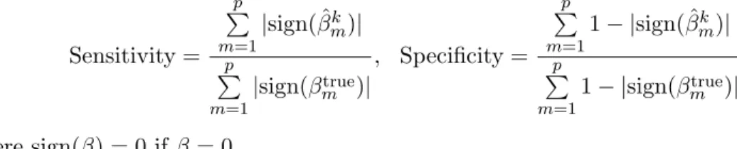
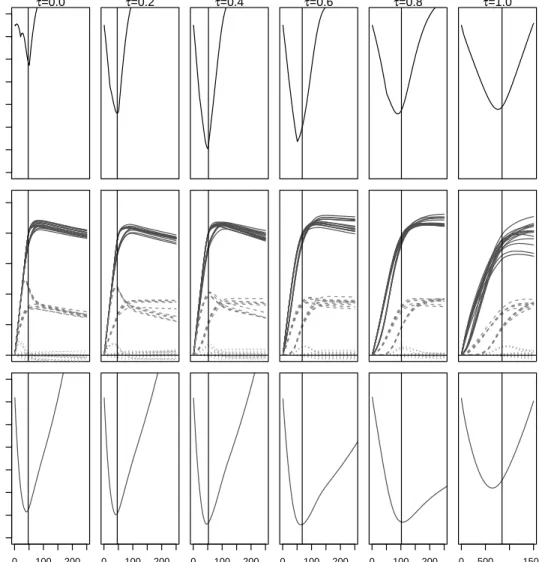
Figure 2.1: AverageL1 distances from the trueβ(top row), estimated coefficient values

(middle row) and MSPE (bottow row) across iterations for various values of τ, when

data are generated from a very sparse true regression model with an intra-individual

correlation ofρ= 0.3. The solid, dashed, and dotted lines in the coefficient plots (middle

row) represent coefficients with true values of 0.5, 0.2, and 0.0 respectively. Results are based on 1000 simulations, each with 500 ThrEEBoost iterations. The solid vertical lines show the iteration where the minimum mean squared error is achieved in each scenario.

(30)

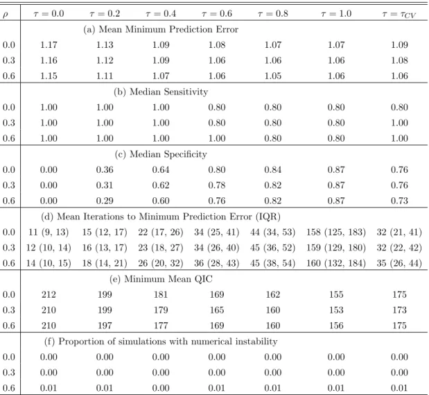
ρ τ = 0.0 τ = 0.2 τ = 0.4 τ = 0.6 τ = 0.8 τ= 1.0 τ=τCV

(a) Mean Minimum Prediction Error

0.0 1.17 1.13 1.09 1.08 1.07 1.07 1.09 0.3 1.16 1.12 1.09 1.06 1.06 1.06 1.08 0.6 1.15 1.11 1.07 1.06 1.05 1.06 1.06 (b) Median Sensitivity 0.0 1.00 1.00 1.00 0.80 0.80 0.80 0.80 0.3 1.00 1.00 1.00 0.80 0.80 0.80 1.00 0.6 1.00 1.00 1.00 1.00 0.80 0.80 1.00 (c) Median Specificity 0.0 0.00 0.36 0.64 0.80 0.84 0.87 0.76 0.3 0.00 0.31 0.62 0.78 0.82 0.87 0.76 0.6 0.00 0.29 0.60 0.76 0.82 0.87 0.73

(d) Mean Iterations to Minimum Prediction Error (IQR)

0.0 11 (9, 13) 15 (12, 17) 22 (17, 26) 34 (25, 41) 44 (34, 53) 158 (125, 183) 32 (21, 41) 0.3 12 (10, 14) 16 (13, 17) 23 (18, 27) 34 (26, 40) 45 (36, 52) 159 (129, 180) 32 (22, 42) 0.6 14 (10, 15) 18 (14, 21) 26 (20, 32) 36 (28, 43) 45 (38, 54) 160 (132, 184) 35 (26, 44)

(e) Minimum Mean QIC

0.0 212 199 181 169 162 155 175 0.3 210 199 179 165 160 153 173 0.6 210 197 177 169 160 156 175

(f) Proportion of simulations with numerical instability

0.0 0.00 0.00 0.00 0.00 0.00 0.00 0.00 0.3 0.00 0.00 0.00 0.00 0.00 0.00 0.00 0.6 0.01 0.01 0.00 0.01 0.01 0.01 0.01

Table 2.1: Mean minimum prediction error (a), median variable selection (b) sensitivity and (c) specificity, (d) mean number of iterations (25th and 75th percentile) to attain minimum prediction error, (e) minimum mean QIC, and (f) proportion of simulations where algorithm did not find a unique minimum MSE for ThrEEBoost in the sparse true

model under different values of the threshold,τ and correlation between intra-individual

observations, ρ. Results are based on 1000 simulations, each with 500 iterations.

by selecting another thresholding value. The proportion of simulation runs resulting in numerical instability are reported in part (f) of Tables 2.1 and 2.2.

(31)

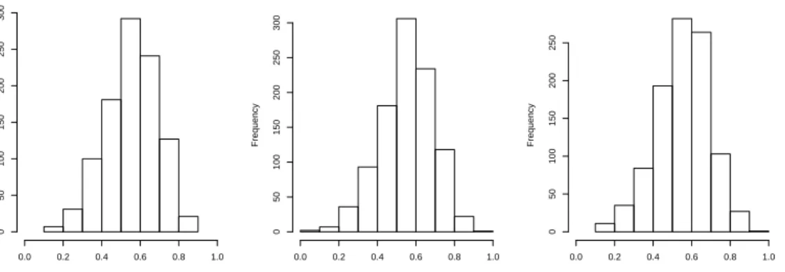
Selection of τ where ρ = 0.0

Cross Validated Threshold Value

Frequency 0.0 0.2 0.4 0.6 0.8 1.0 0 50 100 150 200 250 300 Selection of τ where ρ = 0.3

Frequency 0.0 0.2 0.4 0.6 0.8 1.0 0 50 100 150 200 250

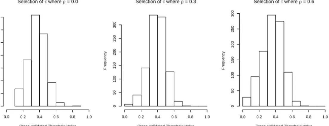
Figure 2.2: The distribution of selected τ values via cross-validation. For each value of

ρ, the medianτCV selected was 0.58.

However, values of τ ≥ 0.6 resulted in very similar MSEs. ThrEEBoost had similar

median sensitivity to EEBoost across values of ρ. For each value of ρ, the sensitivity

ranged from 0.80 to 1.00. Specificity increased with τ, ranging from 0 for τ = 0 to

0.87 for τ = 1. ThrEEBoost with τ < 1 reached minimum MSPE with considerably

fewer iterations than with τ = 1 (i.e., EEBoost). On average, ThrEEBoost with τ <1

located the point on the variable selection path achieving minimum MSPE in 3.5 to 14.4

times fewer iterations than EEBoost. Minimum mean QIC decreased as τ increased.

Figure 2.1 shows the average L1 distance from the true β, coefficient values, and MSE

across the iterations of ThrEEBoost for different τ values in the scenario whereρ=0.3.

Using cross-validation to select an optimal thresholding value τCV, all three cases chose

a median τ of 0.58. The distribution of the chosen τ values are shown in figure 2.2.

The results followed the same patterns for each simulated value of ρ and for each of

(32)

2.3.2 Less sparse regression model with correlated outcomes

Next, we undertook an additional simulation study using the same setup as described in the previous section but with a less sparse true regression model for the mean defined by: βm=            0.5,1≤m≤15 0.2,16≤m≤25 0.0,26≤m≤50

Note that the number of nonzero regression coefficients (25) was nearly equal to the number of independent individuals (30). Due to the reduced sparsity of the model, we increased the number of iterations to 1500 for each of 1000 simulated datasets.

Table 2.2 summarizes the MSPE, QIC, sensitivity, specificity, number of iterations to find minimum MSPE, and rate of numerical instability of the algorithm. For all three

settings of the correlation parameteterρ, mean minimum MSPE and QIC both showed a

clear ”U”-shaped pattern acrossτ. MSPE achieved the lowest value atτ = 0.4, withτ =

0 andτ = 1 yielding MSPE values 6-28% higher than this minimum value. The optimal

τ value to minimize QIC varied from 0.4 to 0.8 depending on ρ. The sensitivity and

specificity results show the trade-off that is at play: sensitivity decreases and specificity

increases as τ goes from 0 to 1. In this case, specificity improves dramatically up to

τ = 0.4 but does not improve substantially with largerτ values; and sensitivity declines

steadily but modestly until τ = 0.6. Figure 2.3 shows the L1 distance from the true β,

the coefficient traceplots, and MSPE across iterations. Figure 2.5 shows the mean QIC

across τ values of 0, 1, andτCV for the variousρ values. The results followed the same

pattern for ρ= 0 andρ= 0.6. Results were also similar in scenarios where the pairwise

(33)

ρ τ= 0.0 τ= 0.2 τ= 0.4 τ= 0.6 τ= 0.8 τ= 1.0 τ=τCV

(a) Mean Minimum Prediction Error

0.0 1.95 1.78 1.65 1.77 2.02 2.12 1.65 0.3 1.53 1.45 1.36 1.42 1.53 1.63 1.35 0.6 1.82 1.71 1.73 1.78 1.86 1.88 1.74 (b) Median Sensitivity 0.0 1.00 0.96 0.92 0.88 0.84 0.80 0.92 0.3 1.00 0.96 0.92 0.88 0.88 0.88 0.92 0.6 1.00 1.00 0.92 0.92 0.92 0.88 0.96 (c) Median Specificity 0.0 0.00 0.24 0.56 0.64 0.68 0.72 0.52 0.3 0.00 0.24 0.56 0.60 0.64 0.64 0.52 0.6 0.00 0.24 0.56 0.60 0.60 0.68 0.52

(d) Mean Iterations to Minimum Prediction Error (IQR)

0.0 40 (40, 51) 43 (44, 50) 49 (49, 58) 63 (59, 79) 88 (73, 116) 696 (213, 966) 53 (49, 59) 0.3 47 (46, 52) 46 (46, 51) 52 (51, 58) 68 (63, 79) 102 (93, 120) 845 (871, 980) 55 (50, 61) 0.6 43 (45, 54) 42 (46, 51) 45 (49, 58) 59 (58, 76) 89 (83, 117) 767 (834, 1000) 53 (49, 59)

(e) Minimum Mean QIC

0.0 340 314 295 317 354 378 296 0.3 334 319 287 287 299 391 282 0.6 470 470 460 458 418 536 487

(f) Proportion of simulations with numerical instability

0.0 0.14 0.10 0.04 0.07 0.10 0.12 0.07 0.3 0.02 0.02 0.01 0.01 0.01 0.03 0.01 0.6 0.03 0.02 0.02 0.02 0.04 0.03 0.03

Table 2.2: Mean minimum prediction error (a), median variable selection (b) sensitivity and (c) specificity, (d) mean number of iterations (25th and 75th percentile) to attain minimum prediction error, (e) minimum mean QIC, and (f) proportion of simulations where algorithm did not find a unique minimum MSE for ThrEEBoost in the less

sparse true model under different values of the threshold, τ, and correlation between

intra-individual observations,ρ. Results are based on 1000 simulations, each with 1500

(34)

3 4 5 6 7 8 9 10 τ=0.0 L1 Distance 0.0 0.1 0.2 0.3 0.4 0.5 β 0 100 200 1.5 2.0 2.5 3.0 3.5 4.0 4.5 5.0 Iterations A v er

τ=0.2 0 100 200 Iterations τ=0.4 0 100 200 Iterations τ=0.6 0 100 200 Iterations τ=0.8 0 100 200 Iterations τ=1.0 0 500 1500 Iterations A v er

β

L

1

Distance

Iterations

Figure 2.3: AverageL1 distances from the trueβ(top row), estimated coefficient values

(middle row) and MSPE (bottow row) across iterations for various values of τ, when

data are generated from a less sparse true regression model with an intra-individual

correlation ofρ= 0.3. The solid, dashed, and dotted lines in the coefficient plots (middle

row) represent coefficients with true values of 0.5, 0.2, and 0.0 respectively. Results are based on 1000 simulations, each with 1500 ThrEEBoost iterations. The solid vertical lines show the iteration where the minimum mean squared error is achieved in each scenario.

(35)

Selection of τ where ρ = 0.0

Frequency 0.0 0.2 0.4 0.6 0.8 1.0 0 50 100 150 200 250 300 350 Selection of τ where ρ = 0.3

Frequency 0.0 0.2 0.4 0.6 0.8 1.0 0 50 100 150 200 250 300

Figure 2.4: The distribution of selected τ values via cross-validation. For each value of

ρ, the medianτCV selected were 0.38, 0.40, and 0.38.

0 200 400 600 800 1000 300 400 500 600 700 800 ρ=0.0 Iterations A v er age QIC 0 200 400 600 800 1000 ρ=0.3 Iterations 0 200 400 600 800 1000 ρ=0.6 Iterations τ 0.0 1.0 τCV

Figure 2.5: Average QIC when data are generated from a less sparse true regression

model with an intra-individual correlation of ρ= 0.3. Results are based on 1000

simu-lations, each with 1500 ThrEEBoost iterations.

Using cross-validation to selectτ offered an improvement over EEBoost (i.e.,

ThrEE-Boost with τ = 1). The MSPE shrunk by about 22%, 18%, and 7% for the cases where

ρ=0.0, 0.3, and 0.6, respectively. The median τ selected was lower than in the sparse

case with values of 0.38, 0.40, and 0.38, respectively. The distributions ofτCV are shown

(36)

2.4

Data application - Box Lunch Study

We illustrate the application of ThrEEBoost to outcome data from the Box Lunch Study, a randomized controlled trial to evaluate the effect of portion size availability on caloric intake and weight gain (French et al., 2014). Two hundred and thirty-three eligible individuals were randomized to one of four groups: three “free lunch” groups and a “no free lunch” group which served as a control. The three “free lunch” conditions differed according to the number of calories provided in the daily box lunch: 400, 800, and 1600.

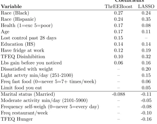
Coefficients

Variable ThrEEBoost LASSO

Race (Black) 0.27 0.24

Race (Hispanic) 0.24 0.35

Health (1=exc 5=poor) 0.17 0.08

Age 0.17 0.11

Lost control past 28 days 0.15 –

Education (HS) 0.14 0.14

Have fridge at work 0.12 0.19

TFEQ Disinhibition 0.10 0.32

Lbs gain before you noticed 0.06 0.16

Dissatisfied with weight – 0.20

Light actvty min/day (251-2100) – 0.15

Freq fast food (0=never 5=7+ times/week) – 0.06

Limit food you eat – 0.05

Marital status (Married) -0.088 -0.11

Moderate activity min/day (2101-5900) – -0.05

Frequency self-weigh (0=never 5=every day) – -0.08

Freq restaurant/week – -0.10

TFEQ Hunger – -0.16

Table 2.3: Coefficients for the optimal ThrEEBoost (τ = 0.4) and LASSO models

selected by cross-validated MSE. Small coefficients (magnitude < 0.05) are omitted.

“–” indicates that the variable was not selected in the model.

Here, we explore the factors associated with BMI in the “no free lunch” group

(37)

ThrEEBoostτ

0 0.2 0.4 0.6 0.8 1.0 LASSO

CV MSE 0.72 0.78 0.60 0.66 0.66 0.75 0.83

Table 2.4: Estimated mean squared prediction error for ThrEEBoost and LASSO mod-els. (CV MSE) denotes models selected by minimizing cross-validated MSE.

points (baseline, 1, 3, and 6 months). There were 54 covariates of interest, including demographic (e.g. age, gender, race, height, education), lifestyle (e.g. smoking sta-tus, physical activity levels), and psychosocial (e.g. frequency of self-weighing, degree of satisfaction with current weight) covariates recorded at baseline, and a variety of longitudinally-recorded food-related outcomes such as average daily caloric intake and average daily servings of fruits and vegetables. The outcome and predictors were scaled to have zero mean and unit variance prior to analysis.

ThrEEBoost was applied using the Gaussian Generalized Estimating Equations

with an exchangeable working correlation structure. The algorithm was run for τ =

0,0.2,0.4,0.6,0.8,and 1, and the optimal model for eachτ was selected as the one which

minimized the MSPE estimated by five fold cross-validation. The smallest MSPE

over-all (0.60) was achieved by ThrEEBoost with τ = 0.4. To implement the LASSO, least

angle regression (LARS) was utilized over five fold cross-validation to select an optimal penalty parameter which minimized the MSPE. Fitting the optimal LASSO model on the full data set, we obtained MSPE of 0.83. The non-zero coefficients for this model are summarized in Table 2.3, and compared to the coefficients from the LASSO fit with smallest cross-validated MSPE. The models selected by LASSO and ThrEEBoost share some covariates in common, but remain quite distinct. Overall, the ThrEEBoost model is more parsimonious than the LASSO model. Notably, the LASSO estimates relatively large coefficients for some variables (e.g., Dissatisfied with weight) which are not selected by ThrEEBoost. This may be due to the fact that the LASSO ignores the correlated nature of the outcome, and is therefore overly optimistic about the amount of

(38)

statistical signal present in the data. Figure 2.6 summarizes the coefficients of the

opti-mal ThrEEBoost model for various values of the threshold parameterτ. The estimated

coefficients forτ = 0.4,0.6,0.8,and 1 are generally similar, with higherτ values leading

to slightly more parsimonious models. However, as shown in Table 2.4, these subtle differences can yield very different prediction errors, hence the path diversity offered by ThrEEBoost is an asset.

2.5

Discussion

We have introduced a thresholded extension of the EEBoost algorithm, ThrEEBoost, and critically assessed its operating characteristics in variable selection and prediction in high-dimensional models. We have shown via a detailed simulation study that ThrEE-Boost provides a predictive advantage over EEThrEE-Boost. In cases when the true regression model was relatively sparse, ThrEEBoost required considerably fewer iterations than EEBoost to locate models with comparable performance. When the regression model was less sparse, varying the thresholding parameter in ThrEEBoost allowed for the ex-ploration of a larger set of variable selection paths, leading to the discovery of models with lower MSPE.

Several limitations of the present study should be acknowledged. This simulation study focused solely on cases of normally distributed correlated outcome data, using GEE with an exchangeable working correlation. Further research is needed to clarify the benefits of thresholded variable selection with other correlation structures, and for other classes of estimating equations. Second, while the numerical experiments are promising, we have not provided theoretical results that guarantee, e.g., that ThrEEBoost possesses

an oracle property. In ongoing work, we are exploring these theoretical properties

of ThrEEBoost and clarifying its relationship to “hybrid” penalized variable selection procedures such as the elastic net.

(39)

τ =0 τ =0.2 τ =0.4 τ =0.6 τ =0.8 τ =1 age height hispanic raceasian raceblack genhealth eversmkr atelgamt0 lostcontrol0 foodfridge0 female ed.highschool ed.somecollege ed.college ed.graduate marital.married income month ripctfat bfastkcal lunchkcal dinnerkcal snackkcal srvgfv srvgssb kcal24h minsed minlgt minmod minvig limitfood.days longfast.days binge judgeweight judgeshape dissatisfiedweight dissatisfiedshape weighfreq lbsnotice lbsdosmthng freqff eatconvenfq eatrstrntfq foodlocker foodroom t1factor t2factor t3factor

Figure 2.6: Coefficient magnitudes for the optimal models (chosen by cross-validated

MSE) for different values of τ. Each row corresponds to a different variable; darker

shades of gray correspond to higher coefficient magnitudes. The names of the variables are displayed on the right; a data dictionary giving the variable descriptions is provided in the Supplementary Materials.

(40)

2.6

Supplementary Materials

Simulation R Code: The R code for the simulation study. (sim threeboost.R, R file)

Data Application R code: The R code to analyze data from the Box Lunch Study. (BLS analysis 06-09-16.R, R file)

ThrEEBoost R Package: The R package which implements ThrEEBoost is available on the Comprehensive R Archive Network (CRAN). The most up-to-date version

of the threeboost package is available athttps://www.github.com/jwolfson/

(41)

Chapter 3

MEBoost

3.1

Introduction

Variable selection is a well-studied problem in situations where covariates are measured without error. However, it is common for covariate measurements to be error-prone or subject to random variation around some mean value. Consider, for instance, a study wherein subjects report their daily food intake on the basis of a dietary recall questionnaire. There is variation from day to day in an individual’s calorie consumption, but it is also well established in the nutrition literature that there is error associated with the recall or measurement of the number of calories in a meal (Spiegelman et al., 1997; Fraser and Stram, 2012). In the usual regression setting, ignoring measurement error leads to biased coefficient estimation (Rosner et al., 1992), and hence the presence of measurement error has the potential to affect the performance of variable selection procedures.

There has been relatively little research done about variable selection in the presence of measurement error. Sørensen et al. (2012) introduced a variation of the Lasso that allows for Normal, i.i.d., additive covariate measurement error. Datta and Zou (2017) proposed the convex conditioned Lasso (CoCoLasso) which corrects for both additive

(42)

and multiplicative measurement error in the normal case. Both of these methods are applicable to linear models for continuous outcomes, but do not easily extend to regres-sion models for other outcome types (e.g., binary or count data). Meanwhile, there is a sizable statistical literature on methods for performing estimation and inference for low-dimensional regression parameters in the presence of measurement error (Rosner et al., 1992; Stefanski and Carroll, 1985; Fuller, 1987), but these approaches do not address

the variable selection problem and cannot be applied in large p, small n problems.

We propose a novel method for variable selection in the presence of measurement error, MEBoost, which leverages estimating equations that have been proposed for low-dimensional estimation and inference in this setting. MEBoost is a computationally efficient path-following algorithm that moves iteratively in directions defined by these estimating equations, only requiring the calculation (not the solution) of an estimat-ing equation at each step. As a result, it is much faster than alternative approaches involving, e.g., a matrix projection calculation at each step. MEBoost is also flexible: the version that we describe is based on estimating equations proposed by Nakamura (Nakamura, 1990), which apply to some generalized linear models, and the underly-ing MEBoost algorithm can easily incorporate measurement error-corrected estimatunderly-ing equations for other regression models. We conducted a simulation study to compare MEBoost to the Convex Conditioned Lasso (CoCoLasso) proposed by Datta and Zou (2017) and the “naive” Lasso which ignores measurement error. We also applied ME-Boost to data from the Box Lunch Study, a clinical trial in nutrition where caloric intake across a number of food categories was based on self-report and hence measured with error.

(43)

3.2

Background

3.2.1 Regression in the Presence of Covariate Measurement Error Our discussion of measurement error models draws heavily from Fuller (1987). When modeling error the covariates can be treated as random or fixed values. Structural models consider the covariates to be random quantities and functional models consider the covariates to be fixed (Buonaccorsi, 2010). We consider a structural model. Let

Y =Xβ+, whereX is a (random) matrix of covariates of dimensionn×p,β a vector

of coefficients of length p, is a vector of Normally distributed i.i.d. random errors

of length n, and Y is the resultant outcome vector also of length n. In an additive

measurement error model, we assume that what is observed is not X but rather the

“contaminated” or “error-prone” matrix W=X+UwhereU a randomn×pmatrix.

When a model is fit that ignores measurement error, i.e. it assumes that the true

model isY =WβW+, the resulting estimatesβˆW are said to benaive and satisfy

E[βˆ0_W] =β0(ΣXX+ ∆)−1ΣXX (3.1)

where β is the true coefficient vector, ΣXX is the covariance matrix of the covariates

and ∆≡ΣU U is the covariance matrix of the measurement error. In the case of linear

regression with a single covariate, (3.1) simplifies to an attenuating factor that biases the coefficient estimates towards zero. However, with multiple covariates the bias may increase, decrease, and even change the sign of the estimated coefficients. Notably, measurement error affecting a single covariate can bias coefficient estimates in all of the covariates, even those that are not measured with error (Buonaccorsi, 2010).

3.2.2 Variable selection in the Presence of Measurement Error

(44)

variable selection in parametric and semi-parametric settings. Focusing on the para-metric setting, they proposed a wide scoping method that can be used in more than just generalized linear models. The method relies on deriving the full likelihood of each

observation and it’s corresponding score function, S_{ef f}∗ (Wi,Yi, β), choosing a penalty

function and finding its derivative, p0(β), then solving the penalized estimating

equa-tions:

n

X

i=1

S_{ef f}∗ (Wi,Yi, β)−np0(β) = 0 (3.2)

Solving the penalized equations can be very difficult computationally, especially in the high dimensional setting. Therefore, we will look to compare our method with faster methods that are variants of the Lasso, which can be solved much more quickly.

3.2.3 Lasso in the Presence of Measurement Error

Sørensen et al. (2012) analyze the Lasso (Tibshirani, 1996) in the presence of measure-ment error by studying the properties of

ˆ βLasso,λn = argmin α ||Y−Wα||2₂+λn||α||1 . (3.3) ˆ

βLasso,λn is asymptotically biased when λn/n → 0 as n → ∞ since E[βˆ

0

Lasso,λn] =

β0(ΣXX+ ∆)−1ΣXX. Notice this is the same bias that is introduced when naive linear

regression is performed on observed covariates. Sørensen et al. (2012) derive a lower bound on the magnitude of the non-zero coefficient elements below which the

corre-sponding covariate will not be selected, and an upper bound on theL1 estimation error

||βˆW−β||1. They show that with increasing measurement error the lower bound

in-creases, i.e., increasing measurement error adds non-informative noise to the system and so for the signal associated with the relevant covariates to be identified the signal must

(45)

increase. Increased measurement error also leads to an increase in the upper bound of the estimation error. Sign consistent selection is also impacted by the presence of co-variate measurement error. Sørensen et al. (2012) set a lower bound on the probability

of sign consistent selection in this setting. The result requires that the

Irrepresentabil-ity Condition with Measurement Error (IC-ME) holds. The IC-ME requires that the measurements of the relevant and irrelevant covariates have limited correlation, relative to the size of the relevant measured covariate correlation. Note the sample correlation of the irrelevant covariates is not considered. By studying the form of the lower bound, it can be concluded that (at least when using the Lasso) measurement error introduces a greater distortion on the selection of irrelevant covariates than it does in the selection of relevant covariates.

Sørensen et al. (2012) introduced an iterative method to obtain the Regularized Corrected Lasso with constraint on the radius R:

ˆ

βRCL= arg min

||β||1<R

{||y−W β||₂−nβ0∆β+λ||β||₁}. (3.4)

The main results of their simulation study were consistent with their analytical results, namely that the corrected Lasso had a slightly lower selection rate for the true covariates than the naive Lasso, but was also more conservative in including irrelevant covariates.

Further, the prediction error, as measured by both ||βˆ−β||1 and ||βˆ−β||2, was lower

for the corrected Lasso.

The major drawback of the corrected Lasso method is that it is very computationally intensive, involving an iterative calculation where each step involves a projection of an

updated ˆβonto theL1-ball for a given radius R. The iterative process must be conducted

for each fixed value of the radius R. The selected values of R provide a path of possible

solutions for ˆβRCL. Hence, the approach seems impractical for large-scale problems and

(46)

3.2.4 The Convex Conditioned Lasso (CoCoLasso)

A recent paper by Datta and Zou (2017) proposes an alternative approach which they refer to as the Convex Conditioned Lasso (CoCoLasso). Consider the following refor-mulation of the Lasso problem,

ˆ βL(λ) = arg min β 1 2β 0 Σβ−ρ0β+λ||β||₁. (3.5)

The CoCoLasso is based on the Loh and Wainwright (2012) corrections for the

predictor-outcome correlation ρ and variance matrix Σ in the presence of measurement error.

When error-prone covariates W are measured in place of X, we can get corrected

estimates ˜ρ and ˆΣ: ˜ ρ= 1 nW 0 Y Σ =ˆ W0W−∆ (3.6)

where ∆ is the (assumed known) variance in the measured W. These estimators are

unbiased. A measurement error corrected Lasso estimate could then be derived by

substituting ˜ρand ˆΣ into (3.5). The problem with this idea is that the corrected matrix

ˆ

Σ may not be a valid covariance matrix, since it is possible to be non positive

semi-definite. If ˆΣ has a negative eigenvalue, then this Lasso function would be non-convex

and unbounded. To overcome this obstacle, the key to the CoCoLasso (Datta and Zou,

2017) is calculating the projection of ˆΣ onto the space of positive definite matrices:

( ˆΣ)+= arg min

Σ≥0

||Σˆ −Σ||_max. (3.7)

The CoCoLasso then solves a standard Lasso problem in which ˆΣ andρ with the

cor-rected values from (3.6) and (3.7), yielding the CoCoLasso estimator:

ˆ βC(λ) = arg min β 1 2β 0 ( ˆΣ)+β−ρ˜ 0 β+λ||β||1. (3.8)

(47)

When ˆΣ is not positive definite, the projection from (3.7) can be challenging to compute. However, the projection only needs to be done once, unlike the Sørensen et al. (2012) correction which requires a projection at each iteration.

3.3

MEBoost: Measurement Error Boosting

Our proposed variable selection algorithm, MEBoost (MeasurementErrorBoosting), is

based on an iterative functional gradient descent type algorithm that generates variable selection paths. The key idea is that, instead of following a path defined by the gradient of a loss function (e.g., the likelihood), the “descent” follows the direction defined by

an estimating equation g(Y,X, β). The algorithmic structure of MEBoost is shared

with ThrEEBoost (Thresholded Estimating Equation Boost, Brown et al. (2017)), a general-purpose technique for variable selection based on estimating equations. While ThrEEBoost described an approach to performing variable selection in the presence of correlated outcomes by leveraging the Generalized Estimating Equations (Liang and Zeger, 1986), MEBoost achieves improved variable selection performance in the pres-ence of measurement error by following a path defined by a measurement error corrected score function due to Nakamura which is described in Section 3.3.1. Nakamura’s ap-proach is applicable to linear regression models with normal additive or multiplicative measurement error. Closed-form corrected score functions are also derived for Poisson, Gamma, and Wald regression. Nakamura comments that no closed form correction can be created for logistic regression. By using this family of corrected score functions, the MEBoost algorithm is more broadly applicable than the corrected Lasso and CoCoLasso, neither of which is obviously generalizable beyond linear regression.

(48)

3.3.1 Corrected Score Function

Nakamura (1990) proposed a set of corrected score functions for performing estimation and inference in the generalized linear regression model where covariates are subject to additive measurement error with known variance matrix ∆. In general, the corrected

score function S* based on the covariates measured with error (W), has the expectation

equal to the score function, S, based on the true covariates (X). For the normal linear

model, Nakamura proposed the following correction to the negative log-likelihood to account for measurement error:

l∗(Y,W, β)0 =−n 2log(2π)−nlog(σ)− 1 2σ2 X [(yi−β0wi)2−β0∆β] (3.9)

Differentiating (3.9) with respect toβ, we obtain the corrected score function:

S∗(Y,W, β)0 =S(Y,W, β)0 +nσ−2β0∆. (3.10)

In this case the corrected score function is the ’naive’ score function, S(Y,W, β)0,

with a measurement error correction determined by the sample size, model error,

mea-surement errors, and the coefficient value: nσ−2β0∆. The naive score function is the

score function from the true model calculated with the measured covariates:

S(Y,W, β, σ) =σ−2W0Y−W0Wβ (3.11)

The corrected variance estimate will be calculated as ∂l∗/∂σ = 0, which in the normal

case is:

ˆ

σ2 =n−1(Y−Wβ∗)0(Y−Wβ∗)−β∗0∆β∗. (3.12)

(49)

variance estimate, n−1₍_Y₋_W_β∗₎0₍_Y₋_W_β∗_{), with a measurement error correction.}

The correction reduces the estimated variance, thus subtracting the noise introduced by the measurement error. In the variance case the correction factor is determined only by the true coefficient vector and the measurement error variance.

As another example, the correction for Poisson distributed data is the following:

S(Y,W, β) =X[ykwk−(wk−∆β)exp(β0wk−β0∆β/2)] (3.13)

which we apply in our data application (see Section 3.5). Nakamura (1990) also pro-vides corrections for multiplicative measurement error in linear regression, as well as measurement error in Gamma and Wald regression. In what follows, we use the nor-mal linear additive measurement error corrected score function as part of an iterative path-following algorithm that performs variable selection in the presence of covariate measurement error.

3.3.2 The MEBoost Algorithm

Our proposed variable selection algorithm, MEBoost, consists of applying ThrEEBoost with the corrected score function and corrected variance estimate described in the pre-vious section. Algorithm 5 summarizes the MEBoost procedure.

Let τ ∈ [0,1] be the fixed thresholding parameter. Starting with a β estimate of

0 and a ˆσ2 = 1, the corrected score function S∗ is calculated at these values, and the

magnitude of each component of ν≡S∗ is recorded. The indices of elements to update

are identified by a thresholding rule, Jt = {j : |νj| ≥ τ ·maxj|νj|}. The next point

in the variable selection path, β(1), is obtained by adding a small value, γ, to each of

these elements in the direction corresponding to the signs of each νj for j ∈ Jt. This

updated β(1) is used to calculate an updated corrected σ2(1). The algorithm continues

(50)

Algorithm 5 MEBoost procedure MEBoost Setβ(0) =0 Setσ2,(t=0) = 1 for t= 0, . . . , T do Compute ν=S∗(Y,W,β)_β =β(t−1) Identify Jt={j:|νj| ≥τ ·maxj|νj|} for alljt∈Jtdo Update β(_jt_t) =β_j(t_t−1)+γ sign(νjt) Setσ2,(t) ₌_n−1 _Y₋_W_β(t)0 Y−Wβ(t) −β(t)0_∆_β(t)

The parametersγ,T and τ interact to determine the specific variable selection path

that results from the algorithm. The smaller the value of γ the smaller the distance

between β estimates on the selection path, while a larger value of γ leads to larger

jumps in the selection path. Ideally, a very small value of γ (e.g., 0.01). would be used,

but if ||β||1 is large, a large number of iterations, T, may be required to generate a

selection path. This of course is the trade-off one is required to make when determining the step size. A selection path incremented by only a small value is preferable to a path which takes large steps, but the time required for a large number of iterations

may become prohibitive. With each of the titerations those elements of the coefficient

vector that are still of size zero have not been selected at this iteration. A conservative

selection approach takes a combination of small γ and T, whereas a more aggressive

approach takes a combination of larger value γ and T. In the case when τ = 1, the

MEBoost algorithm only updates the element(s) with the maximum absolute value. For

any combination of γ and T, this is the most conservative approach that can be taken

and will lead to sparser models than when a threshold is considered. It also requires a

much larger value ofT.

The parameterτ determines how many coefficients are updated at each iteration; it

(51)

to standard gradient descent) and updating only the coefficient corresponding to the

element of the estimating equation with largest magnitude (τ = 1). In the context

of Generalized Linear Models without measurement error, Wolfson (2011) showed that

settingτ = 1 yields an update rule that is asymptotically equivalent (asT → ∞,γ →0,

andT·γ →0) to following the path of minimizers of anL1-penalized projected artificial

log-likelihood ratio whose tangent is the GLM score function. In the case when τ = 1,

the MEBoost algorithm only updates the element(s) with the maximum absolute value.

For any combination of γ and T, this is the most conservative approach that can be

taken and will lead to sparser models than when a threshold is considered. It also

requires a much larger value of T. By allow

Variable Selection and Prediction in Messy'' High-Dimensional Data"