Worcester Polytechnic Institute
Digital WPI
Doctoral Dissertations (All Dissertations, All Years) Electronic Theses and Dissertations
2015-10-13
Developing and validating Fuzzy-Border
continuum solvation model with POlarizable
Simulations Second order Interaction Model
(POSSIM) force field for proteins
Ity Sharma
Worcester Polytechnic Institute
Follow this and additional works at:https://digitalcommons.wpi.edu/etd-dissertations
This dissertation is brought to you for free and open access byDigital WPI. It has been accepted for inclusion in Doctoral Dissertations (All Dissertations, All Years) by an authorized administrator of Digital WPI. For more information, please [email protected].
Repository Citation
Sharma, I. (2015).Developing and validating Fuzzy-Border continuum solvation model with POlarizable Simulations Second order Interaction Model (POSSIM) force field for proteins. Retrieved fromhttps://digitalcommons.wpi.edu/etd-dissertations/393
1
Developing and validating Fuzzy-Border continuum solvation model
with POlarizable Simulations Second order Interaction Model
(POSSIM) force field for proteins
by
Ity Sharma
A Dissertation Submitted to the Faculty
of the
WORCESTER POLYTECHNIC INSTITUTE in partial fulfillment of the requirements for the
Degree of Doctor of Philosophy in
Chemistry 2015
2
ACKNOWLEDGEMENTS
The completion of this dissertation has been a long journey and could not have been possible without the help and support of my family and friends.
First and foremost I would like to express my deepest gratitude to my advisor Professor George A. Kaminski for providing me an opportunity to work in his research group and making my Ph.D. experience very productive. I would like to thank him for not only mentoring and encouraging me to pursue my goals but also allowing me to grow as an independent thinker. Many thanks to the members of the Kaminski research group, both past and present, for their years of friendship, help and technical support; Qina Sa, Dr. Xinbi Li, John Peter Cvitkovic, Dr. Sergei Y. Ponomarev, Dr. Timothy Click and Dr. Haijun Yang. They immensely supported towards my intellectual development. I am also thankful to Zhen Chen, Zijian Xia, Daniel Sigalovsky and Anetta Goldsher, for all their support during their undergraduate research in Dr. Kaminski group. I am also thankful to Siamak M Najafi for making sure that my computer and software ran smoothly.
I would like to thank my PhD dissertation committee, Prof James P. Dittami, Prof John C. MacDonald and Prof Erkan Tuzel for their time, valuable suggestions and guidance. Special thanks is reserved for late Prof Robert E Connors for his enormous support, valuable suggestions and guidance during my first year seminar, second year qualifier and as my TA advisor.
I am especially grateful to Prof Arne Gericke for all his help as the head of the department and
Prof Kristin K. Wobbe for her valuable suggestions during very critical time of my graduate studies.
I am also very thankful to Prof Uma Kumar, Prof Glazer, Prof Wen-Chao Lai, Prof Drew Brodeur, Prof Destin Heilman and Prof Sal Triolo for all they have taught me to become a better TA. Thanks also go out to Mary, Rebecca and Paula for theirtremendous help during my TA duties. Special thanks to Ann Mondor for always being there no matter the task or circumstance.
3
I owe a special thanks to Ms. Shobha Reddy, Dr. Varnitha Reddy and Dr. Sarva Lakshmi for their friendship and support throughout my graduate studies at WPI.
I would like to acknowledge the Chemistry and Biochemistry department at Worcester Polytechnic Institute for the financial support and assistantship during my course of graduate studies.
I am also thankful to WPI for the financial support I recieved from the Backlin Fund for the Fall Semester 2015.
The PhD dissertation, which I completed at Worcester Polytechnic Institute, was indeed one long journey.
My time at the University of Connecticut was brief but forever memorable. The friendships made with Dupinderjeet Kaur Mann, Kalpanie Bandara, Narendran Gummudipundi D and Sang-Yong Ju in the beautiful campus of UConn will last forever. UConn offered me the opportunity to work with an outstanding professor, Fotios Papadimitrakopoulos who taught me the value of hard work.
I will always be very grateful to the Department of Chemistry, Guru Nanak Dev University (GNDU), Amritsar, India from where this quest for knowledge began. I am thankful to my professors at GNDU for their encouragement and guidance. I am also grateful to my friends in
GNDU for their contribution to my personal and professional development. No acknowledgments would be complete without my family.
My sincere most gratitude goes out to my parents Kiran Sharma and Janak Raj Sharma, without whom none of my success would have been possible. They always believed in me, provided me the best education and made numerous sacrifices to make my life better. I lost my mother a month before joining the graduate program in WPI but I’ve always felt her around me especially when the days were tough and nights were long.
I would also like to thank my sister Upasana Dhillon and brother in law Tanveer Dhillon, for their love, support, and understanding. Similar thanks are reserved for my sister Nidhi Sharma
4
and her husband Amit K. Sharma for their love and understanding. I am also grateful to my younger brother Abhishek Sharma for his support and encouragement. Upasana and Nidhi are not only my sisters but my best friends and their unconditional love has encouraged and motivated me at every step during my graduate studies.
I am also grateful to my mother in law (Kanta Sharma) and father in law (Jaswinder P. Sharma) as well as my brother in law (Amit K Sharma) and his wife Neerja for their love, support and best wishes.
My final, and most heartfelt, acknowledgement goes to my husband and friend Vaneet Kumar Sharma who has supported me in whatever I intended to do and without whom I would have not made it this far. He is source of my courage to take on challenges that have come in the way. The understanding and love we have shared together have helped us in enduring and surviving the experience of graduate school while being parents. Our daughter, Sanjana Sharma is probably the person I owe my success to. She has always been my greatest fan and supporter, reassuring me whenever in doubt. No matter how things look, her smile has always driven me closer to my goals.
Hopefully this thesis would be a roadmap for Sanjana and my nephews Ishaan and Saman so that they understand the value of persistence and education.
5
TABLE OF CONTENTS
CHAPTER 1: Introduction: Force fields and Solvation Models in Biomolecular SimulationsComputational chemistry methods
1.1. Computational Chemistry 13
1.2. Force field 14
1.2.1. Types of force field 16
1.2.2. Methods to include electronic polarization effects in force field 26
1.3. Solvation Models 30
1.3.1. Solvation Free Energy 33
1.3.2. Types of Implicit Solvation Models 35
References 51
CHAPTER 2: Developing and parameterizing first-order Fuzzy-Border (FB) continuum solvation model with OPLS-AA force field and calculating hydration energies of small molecules and pKa of substituted phenols
2.1. Introduction 66
2.2. Methods 70
2.2.1. Force Field – Optimized Potential for Liquid Simulations-All Atom
(OPLS-AA) force field 70
2.2.2. Fuzzy-Border (FB) continuum solvation model 72
2.2.3. The general protocol used in the pKa calculations 84
2.3. Results and discussions 86
2.3.1. Hydration Energies of Benzene, Phenol and Phenoxide and
the Phenol pKa Value 96
2.3.2. pKa Values of the Substituted Phenols and Hydration Energies of
Related Molecules 98
6
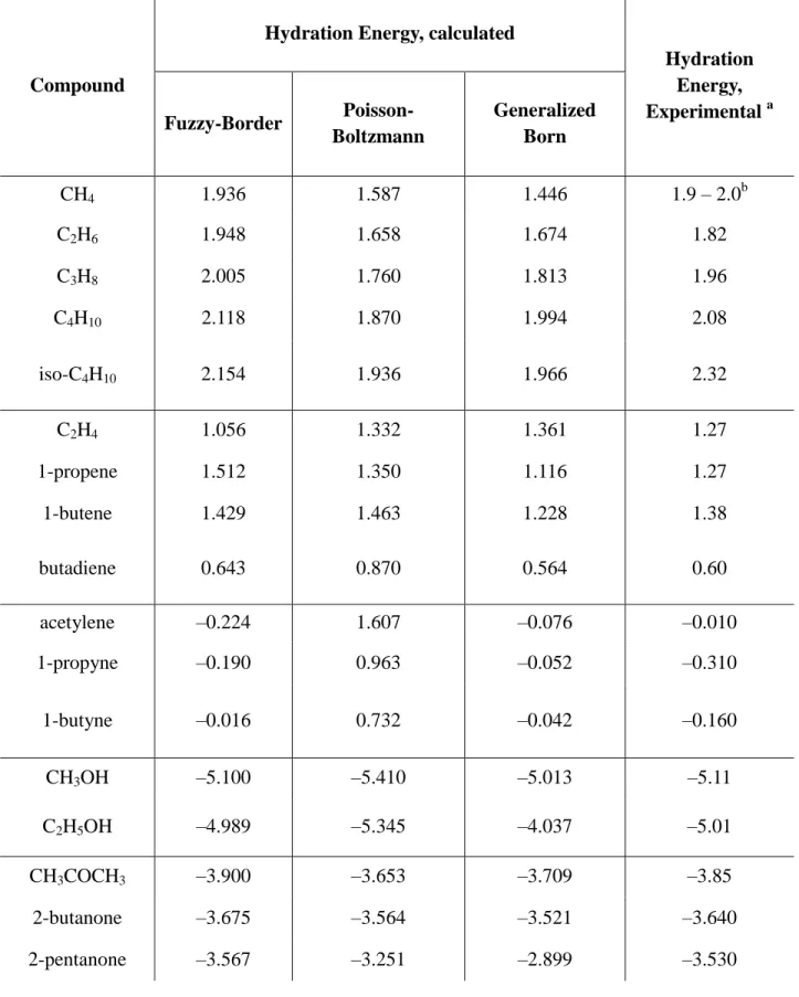
2.3.4. Comparison of Fuzzy-Border Hydration Energies with
Poisson-Boltzmann and Generalized Born Results 111
2.3.5. Absolute Acidity Constants for Propanoic and Butanoic Acids 115
2.4. Conclusions 117
References 118
CHAPTER 3: Developing and parameterizing first-order Fuzzy-Border (FB) continuum solvation model with Polarizable Simulations Second-Order Interaction Model (POSSIM) force field and computing pKa of carboxylic and basic residues of OMTKY3 protein
3.1. Introduction 123
3.2. Methods 128
3.2.1. Polarizable Simulations Second-order Interaction Model 128
3.2.2. Fuzzy-Border Solvation Model 134
3.2.3. General Scheme for pKa calculations of protein residues 139
3.3. Results and discussions 140
3.3.1. POSSIM force field parameterization 140
3.3.2. Fuzzy-Border parameterization 146
3.3.3. pKa values of carboxylic residues of OMTKY3 protein and
hydration energies of related molecules 149
3.3.4. pKa values of basic residues of OMTKY3 protein and
hydration energies of related molecules 156
3.4. Conclusions 166
References 168
CHAPTER 4: Impact of pressure on conformational equlibria of N-acetyl-L-alanine-N'-methylamide in aqueous solution with POlarizable Simulations Second-order Interaction Model (POSSIM) and fixed charge OPLS-AA force field
7
4.2. Methods 177
4.3. Results and Discussions 178
4.3.1. Fixed dihedral angles (ϕ, ψ) at quantum mechanical values
with POSSIM force field 178
4.3.2. Unconstrained dihedral angles (ϕ, ψ) at quantum mechanical
values with POSSIM force field 183
4.3.3. Fixed dihedral angles (ϕ, ψ) at quantum mechanical values
with OPLS force field 186
4.3.4. Unconstrained dihedral angles (ϕ, ψ) at quantum mechanical values
with OPLS force field 188
4.4. Conclusions 192
References 194
CHAPTER 5: Future Directions
5.1. Introduction 198
5.2. Calculation of pKa values of proteins using
polarizable POSSIM force field 199 5.3. Calculation of binding free energy of protein ligand complexes 199 5.4. Applying second order FB model to compute binding affinity
of HIV inhibitors 201
8
ABSTRACT
The accurate, fast and low cost computational tools are indispensable for studying the structure and dynamics of biological macromolecules in aqueous solution. The goal of this thesis is development and validation of continuum Fuzzy-Border (FB) solvation model to work with the Polarizable Simulations Second-order Interaction Model (POSSIM) force field for proteins developed by Professor G A Kaminski. The implicit FB model has advantages over the popularly used Poisson Boltzmann (PB) solvation model. The FB continuum model attenuates the noise and convergence issues commonly present in numerical treatments of the PB model by employing fixed position cubic grid to compute interactions. It also uses either second or first-order approximation for the solvent polarization which is similar to the second-first-order explicit polarization applied in POSSIM force field.
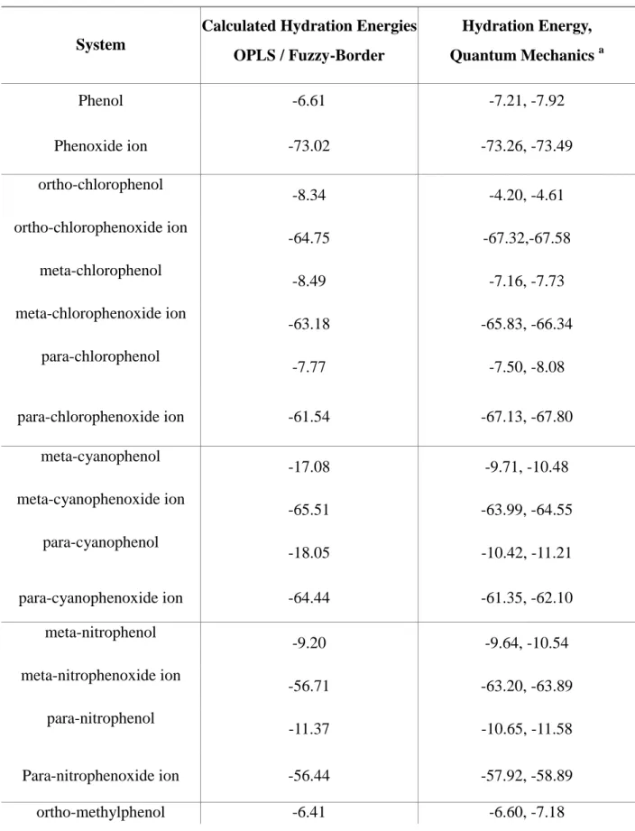
The FB model was first developed and parameterized with nonpolarizable OPLS-AA force field for small molecules which are not only important in themselves but also building blocks of proteins and peptide side chains. The hydration parameters are fitted to reproduce the experimental or quantum mechanical hydration energies of the molecules with the overall average unsigned error of ca. 0.076kcal/mol. It was further validated by computing the absolute pKa values of 11 substituted phenols with the average unsigned error of 0.41pH units in
comparison with the quantum mechanical error of 0.38pH units for this set of molecules. There was a good transferability of hydration parameters and the results were produced only with fitting of the specific atoms to the hydration energy and pKa targets. This clearly demonstrates
the numerical and physical basis of the model is good enough and with proper fitting can reproduce the acidity constants for other systems as well.
9
After the successful development of FB model with the fixed charges OPLS-AA force field, it was expanded to permit simulations with Polarizable Simulations Second-order Interaction Model (POSSIM) force field. The hydration parameters of the small molecules representing analogues of protein side chains were fitted to their solvation energies at 298.15K with an average error of ca.0.136kcal/mol. Second, the resulting parameters were used to reproduce the pKa values of the reference systems and the carboxylic (Asp7, Glu10, Glu19, Asp27 and Glu43)
and basic residues (Lys13, Lys29, Lys34, His52 and Lys55) of the turkey ovomucoid third domain (OMTKY3) protein. The overall average unsigned error in the pKa values of the acid
residues was found to be 0.37pH units and the basic residues was 0.38 pH units compared to 0.58pH units and 0.72 pH units calculated previously using polarizable force field (PFF) and Poisson Boltzmann formalism (PBF) continuum solvation model. These results are produced with fitting of specific atoms of the reference systems and carboxylic and basic residues of the OMTKY3 protein. Since FB model has produced improved pKa shifts of carboxylic residues and
basic protein residues in OMTKY3 protein compared to PBF/PFF, it suggests the methodology of first-order FB continuum solvation model works well in such calculations. In this study the importance of explicit treatment of the electrostatic polarization in calculating pKa of both acid
and basic protein residues is also emphasized. Moreover, the presented results demonstrate not only the consistently good degree of accuracy of protein pKa calculations with the second-degree
POSSIM approximation of the polarizable calculations and the first-order approximation used in the Fuzzy-Border model for the continuum solvation energy, but also a high degree of transferability of both the POSSIM and continuum solvent Fuzzy Border parameters. Therefore, the FB model of solvation combined with the POSSIM force field can be successfully applied to study the protein and protein-ligand systems in water.
10
ABBREVIATIONS
AIDS Acquired Immunodeficiency Syndrome
AMBER Assisted Model Building and Energy Refinement
AMOEBA Atomic Multipole Optimized Energetics for Biomolecular Simulation
AM1 Austin Model 1
CFF Consistent Force Field
CHARMM Chemistry at HARvard Macromolecular Mechanics
CM1 Compact Model 1
COSMO Conductor–like Screening Model
CVFF Consistent Valence Force Field
DAPY Diarylpyrimidine
DATA Diaryltriazine
DFT Density Functional Theory
DO Drude Oscillator
DPCM Dielectric Polarizable Continuum Model
ECEPP Empirical Conformational Energy Program for Peptides
EQ Electronegativity Equalization
FQ Fluctuating Charge
FTIs Farnesyl Transferase Inhibitors
GAFF Generalized Amber Force Field
GB Generalized-Born
GROMOS GROningen MOlecular Simulation
IEF Integral Equation Formulation
IPD Induced Point Dipole
LJ Lennard-Jones
MC Monte Carlo
MD Molecular Dynamics
11
MMFF Merck Molecular Force Field
MO Molecular orbital methods
MPa MegaPascals
NEMO Non-Empirical Molecular Orbital
NMR Nuclear Magnetic Resonance
NNRTIs Non-Nucleoside Reverse Transcriptase Inhibitors
NRTIs Nucleoside Reverse Transcriptase Inhibitors
OPLS Optimized Potentials for Liquid Simulations
PB Poisson-Boltzmann
PCM Polarizable Continuum Models
PFF Polarizable Force Field
POSSIM Polarizable Simulations Second-order Interaction Model
QM Quantum Mechanics
RISM Reference Interaction Site Model
Rnase Sa Ribonuclease Sa
RT Reverse Transcriptase
SASA Solvent Accessible Surface Area
SDFF Spectroscopically Determined Force Field
SIBFA Sum of Interactions Between Fragments Ab initio computed
TIP4P-FQ Four-site Transferable Intermolecular Potential Model-Fluctuating Charge
UFF Universal Force Field
12
Chapter 1
Introduction: Force Fields and Solvation Models in
Biomolecular Simulations
13
1.1
Computational Chemistry
Computational chemistry has become increasingly significant in study of structure and function of biological macromolecules as well as organic molecules. It is a major tool in investigating areas such as folding and conformational changes of proteins1, protein-protein interaction2, structure-based drug design3, computing binding free energy of ligands4 andmodeling enzyme mechanisms.5
Currently two main methods are used to evaluate energy in theoretical chemistry6:
Quantum Mechanics (QM)
Molecular Mechanics (MM)
Both these computational methods calculate potential energy, the difference being in their approach. Quantum mechanics (QM) calculates the potential energy based on the information of electronic structures and the results can be described as the solutions of the Schrödinger equation. In the case of Molecular mechanics (MM) electrons are not considered explicitly in the molecule although there are some exceptions. The atom and its electrons are treated as a single unit represented by potential energy functions or force fields.
Quantum mechanics (QM) calculations can be further divided in two categories7:
Ab initio
14
Ab initio methods use the Schrödinger equation with approximations to calculate total energy of the system. Such a calculation is based on quantum mechanics only and no experimental data is used. In the case of semiempirical methods the potential energy is calculated using experimental parameters as well as Schrödinger equation.
Quantum mechanics (QM) is generally regarded as the most accurate for potential energy calculations and has been the most popular approach to calculate energy.
However, there are limitations to its applications;
Firstly, QM calculations are computer intensive. They need large computational resources and longer time when dealing with larger systems and thus their area of applications is limited.
Secondly, QM calculations can produce different results when using different levels of theory and this deviation is evident for both small and large systems.
Thus in order to have results which are reasonably accurate, complete within a reasonable computational time and applicable to different molecular systems, molecular mechanics (MM) calculations are performed. Molecular mechanics calculates the potential energy using parameters derived from experimental data or ab inito calculation using force fields.
1.2 Force field
A Force field constitutes a set of analytical potential energy functions derived from classical mechanics. These potential energy functions are used to calculate the energy of a molecular system using parameters derived from the experimental or quantum mechanical techniques such
15
as ab initio, DFT (Density Functional Theory). This combined set of potential energy functions and their parameters is known as a force field.8
The general equation used to calculate energy in a force field consists of the bonded and the non-bonded interactions. The non-bonded energy interactions is a sum of intramolecular bonds, angles and torsion terms and the nonbonded consist of both intermolecular and intramolecular van der Waal and electrostatic Coulomb interaction terms. (Equation (1a) (1b), Figure 1).
(1a) (1b)
Figure 1: Bonded and non-bonded interactions in a molecule
Force fields can be generic or specific depending on their implementation. Force fields such as universal force field (UFF)9 and generalized Amber force field (GAFF)10 are of general applicability but recently developed force fields are more specialized to organic, inorganic or
16
biological molecules. They are more specifically designed for either organic molecules such as sugars or lipids or bio macromolecules such as proteins and nucleic acids.
1.2.1 Types of Force field
Force fields can be grouped under three major classes:
Class I force fields
Class IΙ force fields
Class ΙΙI force fields
Class I force fields:
Force fields such as AMBER11,12, CHARMM13, OPLS14, MMFF15,GROMOS16, ECEPP17 have been successfully applied to address many problems. The functional form of this type of force fields represents minimum forces to describe the molecular structure.
The total energy for bonded interactions consists of harmonic terms for bond stretching, angle bending and a Fourier series for each dihedral angle as shown in equation (2).
(2)
In equation (2), req and θeq represent the equilibrium values for the bond lengths and the angles
17
dihedral phase angle. Kr, Kθ and Vn are the force constants for bonds, angles and the dihedral
terms respectively.
The nonbonded energy term is given as sum of van der Waals and the Coulomb electrostatic interactions between the atoms separated by more than two bonds in both the intramolecular and intermolecular atom pairs (equation (3)). The van der Waals interactions are evaluated by Lennard-Jones (LJ) formalism. The LJ interaction energy term contains the short range repulsive and long range attractive term. For the repulsive term, the energy varies as a function of r-12 whereas for the attractive case it is proportional to r-6 as in London dispersion energy between the two atoms with polarizabilities a (-a2/r6).
(3)
The constant A and B in the first term in equation (3) are the van der Waals coefficients describing interactions for same atom types when the well depth (εi) and atomic radii (Ri) are
known (equation (4) and equation (5)).
(4)
(5)
The electrostatic and van der Waals interactions between the atoms separated by three or more bonds or 1-4 nonbonded interactions are treated separately and their magnitude is often scaled
18
down. This formalism is typical but not the only possible one for class Ι force fields. Some force fields of this type have additional energy terms or small variations in the functional forms.
The equations (2) to (5) contain several constants or parameters that are produced to reproduce the experimental or the quantum mechanically obtained conformational energies and geometries, binding energies, vibrational frequencies, heats of formation, and other properties characterizing the condensed or gas phase.18
The electrostatic interactions in Class Ι force field use pairwise additive potential energy functions in terms of fixed charges, usually centered on atoms. This results in lack of accuracy in calculation of potential energy functions in some cases like treating molecules in environments of different dielectrics. The accuracy of many force fields have been increased by reparameterizing the current set of parameters or parameterizing the complete force field after adding new functional forms as in highly successful OPLS (Optimized Potentials for Liquid Simulations) force field where several improvements have been incorporated in the last thirty years resulting in faster and more accurate liquid simulations for large organic molecules and biomolecules such as proteins. These modifications have resulted in improved predictions of thermodynamic properties from the liquid state such as heat of vaporization, and free energy of hydration.
The limitations due to the use of fixed charges and pairwise additive approximation has led to the development of more improved force fields.
19
Class II force fields:
Class ΙΙ force fields have more complex functional form and includeterms in addition to equations (2)-(5). These are higher-order stretch bend valence terms to treat anharmonicity as well as cross terms between stretch and bend valence and/or bend and dihedral angles.19 Some also include a Morse function that allows for bond breaking in empirical force fields and a cosine angle term for nonlinear angle.11, 20
The nonbonded electrostatic interactions between the point charges are represented by Coulomb formalism for most of the force fields. These point charges are mostly located on the nuclei except in case of MM3 force field where the electrostatic interactions are evaluated as point dipoles on the chemical bonds21. In standard force fields van der Waal interactions are proportional to the distance, R, between the two interacting points and varies as 12-6 (R-12 to R-6) in standard Lennard-Jones interaction energy term. Other alternatives to this term include 9-6 term, buffered 14-7 used in MMFF force field or exponential Buckingham potential22 that are more realistic and expensive to compute. The accuracy of class ΙΙ force fields increase with addition of these terms and is particularly useful for reproducing conformational energies and equilibria, molecular structures and molecular vibrations. Examples of class ΙΙ force field are
CFF,22 CVFF,23 MMFF,24 MM3/MM421,25 and UFF.11
Though Class ΙΙ force fields have been validated over a number of decades and are found to be robust for treating structure and energetics as well in reproducing properties of biological systems, they typically do not perform well in many condensed phase simulations.26 In these simulations the high dielectric medium such as water polarizes the charge distribution of the solute. The molecule of water itself in the gas phase carries a dipole moment of 1.85 Debye and
20
its polarization increases by about one Debye in bulk water. Therefore, the explicit treatment of electrostatic polarization interactions is critical for such simulations. Examples of modeling of protein folding where the section of amino acids form a hydrophobic core and must be transferred from its water environment to the interior of a protein with a different dielectric, folding of RNA in divalent ions media or folding of membrane proteins in a lipid environment all underline the need of explicit polarization effects.27
In both Class Ι and Class ΙΙ force fields the polarization is included implicitly in the averaged manner. It is either included in Lennard-Jones interactions or by assignment of the fixed enhanced partial charges, qi, to the atoms. These partial charges are produced through quantum
mechanical methods, which overestimate the values of charge. These methods treating polarization in an effective manner limits the accuracy of nonpolarizable or Class Ι and Class ΙΙ force fields as the polarization can vary significantly in a biomolecular system extending from the polar environment at the protein surface to the non-polar interior of the protein. The response of charge distribution to the changing dielectric environment can only be accounted for by incorporating explicit polarization effects.
In the Class Ι and Class ΙΙ force fields, molecules do not respond to the changes in the electrostatic environment (temperature, pressure, pH, ion concentration and type of solvent) contrary to the real molecular systems which get perturbed due to the presence of a charged body, thus disturbing its geometry and energetics. Therefore, a major focus is in the development of the force field to treat electrostatic polarization of charge distribution by the environment of different dielectrics.
21
One of the first attempts to treat polarization was undertaken by Warshel and Lewitt in the study of lysozyme reaction in 1976.28 Polarization has also shown to significantly affect intermolecular interactions in the gas-phase environment. Caldwell and Kollman29 publisheddevelopment of a model to study aromatic-cation interactions by including polarization explicitly in additive force fields. Importance of polarization in molecular modeling was further presented by Rick, Stuart and Berne in their study of the hydration of the chloride ion in a small water droplet.30 The chloride ion preferred to remain buried in the center of the droplet using the nonpolarizable OPLS/AA force field whereas with the polarizable water model TIP4P-FQ clearly showed preference of the ion to remain on the surface, hence depicting the entropic effect consistent with experimental evidence.
Thus published reports similar to presented above emphasized the need to include explicitly many-body induced polarization leading to the development of the class III polarizable force fields.
Class III force fields:
Class III force fields are the most recent area of computational research that incorporate explicit polarizability term in the total energy, thus allowing the tuning of charge distribution to the changing dielectric environment.This polarizability or redistribution of charge in response to the changing electric field in molecular simulations is non-additive. The non-additivity arises from the different electron polarization of two atoms in the presence of one or more bonded atoms.22
Examples of Class III force fields are either the ones which have included the polarization term since their inception such as AMOEBA,31 SIBFA,32 SDFF,33 NEMO,34 POSSIM35 or are the counterparts of the existing standard class I force fields for example AMBER ff02,
ff02EP,36 CHARMM,37 PIPF-CHARMM,38 OPLS/PFF,39 OPLS-AAP/OPLS-CM1AP,40 and GROMOS.41
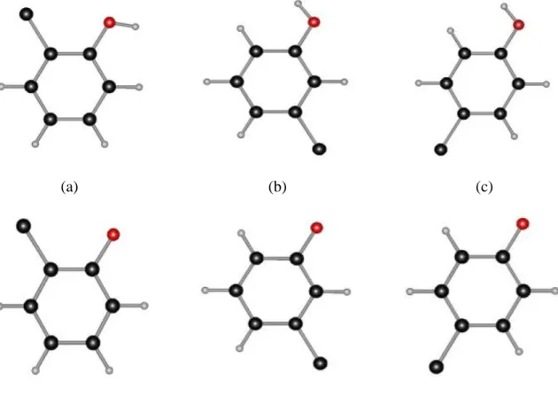
The specific examples illustrating the importance of explicit electrostatic polarizability are evident in the following examples. First is the calculation of accurate binding energies of E-selectin forming a complex with a calcium ion and Sialyl LewisX (Slx). It is known that the surfaces of cancer cells are found to be rich in these sugars. Selectins on the surface of the platelets bind to the Slx carrying cancer cells into the circulatory system. The X-Ray structure of E-selectin-Slx complex reveals a stable complex with two hydrogen bonds between one of the saccharide monomers in Slx, fucose and Ca++ ion, figure 2(a). The energy of formation of the E-selectin-Slx complex was found to be thermodynamically unstable +14.52kcal/mol with the OPLS-AA force field compared to -17.93kcal/mol calculated with the PFF or Polarizable Force Field.39(b), 39(d)
In another example the formation energy of stable complex between protein farnesyl transferase and inhibitor SCH66336 (4-{2-[4-(3,10-dibromo-8-chloro-6,11-dihydro-5H-benzo[5,6]cyclohepta[1,2-B]pyridin-11-yl)piperdin-1-yl]-2-oxoethyl} piperidine-1-carboxamide)43 was studied, figure 2(b). The complex formation energy of this stable complex computed with OPLS-AA force field was +55.84kcal/mol while the polarizable force field
23
(PFF)39(d) calculated a value of -28.04kcal/mol in agreement with the stable protein-inhibitor complex.
Figure 2: Complex of E-selectin and Ca++ with Sialyl Lewis X, PDB 1G1T (a) and SCH66336 (magenta) in complex with farnesyl transferase, PDB 1O5M (b).
It is imperative to include the electrostatic polarization explicitly in calculations such as pKa and
ion binding that involves strong electrostatic interactions as shown by our group. Figure 3 show the calculation of pKa values of carboxylic 42(a) and basic 42(b) OMTKY3 protein residues with
nonpolarizable OPLS-AA and polarizable PFF force fields. The accurate pKa determination of
24
(a)
(b)
Figure 3: pKa values of carboxylic (a) and basic (b) OMTKY3 residues42
Our group has also shown increased accuracy in simulations of ion interactions with small molecules and proteins with a polarizable force field. The Cu(ǀ) complexes with benzene show improved geometry and energy with a polarizable force field (PFF) than the fixed charge OPLS force field shown in the table 1.43 Parameters for copper (ǀ) were refitted with both OPLS and PFF force fields for copper-water gas phase complexes but was observed to work well for the copper complex with benzene. The error in the hydration energy of the copper ion with the PFF was also found to be only 1.8% compared to the OPLS error of 22%.
25
Table1: Energy and distances in complex of Cu(ǀ) with benzene molecule 43
Model systems Energy, kcal/mol Cu+…C(benzene) distance, Å
OPLS -14.0 2.77
OPLS, refitted for TIP3P -25.2 2.14 OPLS, refitted for TIP4P -26.0 2.11
PFF -54.4 2.30
Reference 44 -56.9 to -61.3 2.31
Ion binding calculations were also extended to a Cu+ complex with bacillus subtilis CopZ protein. The binding energy with non-polarizable OPLS an incorrect value of +9.98 kcal/mol while with the polarizable PFF force field was -33.05kcal/mol. The PFF force field also predicts correct Cu+…S- distances within the accuracy of 0.06Å compared to the ca. 0.4Å error with the fixed charge model from the experimental results, figure 4.44
(a) (b)
Figure 4: A fragment of Copz protein -copper (ǀ) complex as simulated with OPLS (a) and PFF (b) force fields 44
26
The above examples emphasize the importance of explicit electrostatic polarization interaction in studying many protein-ligand interactions. Polarization has proven to be significant particularly in computing acidity constants of small molecules and proteins, dimerization energies (aromatic cation interactions), binding energy (such as ion binding with small molecules and protein and sugar protein complexes) and in energetics and/or directionality of formation of hydrogen bonds.
Although the force fields with explicit polarization yield accurate results in many simulations, those force fields require 3 to 10 times greater computing time depending on the system than their additive analogs. This issue has been partially addressed by massive progress made in computer technologies and advancements in programming such as the particle-mesh Ewald (PME) 45 method for accurate and fast calculation of electrostatic energy. As mentioned above the challenge is to accurately evaluate many body interactions in a reasonably time efficient manner. Several methods have been proposed to incorporate electronic polarization in molecular simulations, including fluctuating charges (FQ) as well as Drude oscillator and induced dipole models.
1.2.2 Methods to include electronic polarization effects in force fields
Currently, the basic methods proposed to include the electronic polarization effects in force fields are fluctuating charge (FQ), Drude oscillator (DO) and induced point dipole (IPD) models.46,48
27
Fluctuating charge (FQ) model
46This model is also known as the electronegativity equalization (EQ) model as it allow flow of charges between the atoms to equalize their instantaneous electronegativity. This approach involves assigning fictitious masses to the fluctuating charges (FQs) and treating them as additional degrees of freedom in the equations of the motion. The resulting equations of motions are solved more efficiently in molecular dynamics (MD) simulations than the Monte Carlo (MC) simulations. In the MD simulations, these equations are solved using the extended Lagrangian method47 at the associated computational cost slightly higher than required for the fixed atomic charges of pairwise additive force fields. The parameters in the FQ model used to determine charge and response in polarization can be obtained empirically or fit to reproduce the two-body, three-body quantum chemical energies of water dimers and trimers.
The FQ model has been used to include polarization in the universal force field (UFF)10, PFF39, and CHARMM13 force fields. One disadvantage of this model is the confinement of the polarizability in the molecular plane whereas experimentally it is found to be nearly isotropic.
Drude oscillator (DO) method
48DO models also known as shell models are commonly used in the simulations of solid-state ionic materials and many other systems as well. The electronic polarization is incorporated in this model by representing an atom or ion as a two particle system. The two particles are the core and a shell linked with a harmonic spring and associated with certain fixed charges. This core and shell together is known as a Drude particle. The electronic polarization is linked to the response in the relative displacement of the charges to the external electric field. This approach to add
28
electrostatic polarizability has been incorporated in CHARMM37 and GROMOS41 molecular modeling packages.
Inducible point dipole model
This is the most widely used method to treat molecular polarizability and its applicability varies from atomic to molecular systems such as noble gases to water to proteins. This approach has been used in many force fields such as OPLS/PFF39, AMOEBA31 and AMBER ff02, ff02EP36. Many new water models being developed employ this method to incorporate electronic polarization. According to this model, a point dipole, or PD, is induced at each contributing center in response to the total electric field, E. Hence the total energy, Etotal, includes an
additional energy term, Epol(Equation 6).
(6)
The polarization resulting from the dipolar interactions between the permanent partial charges and the induced dipoles is incorporated in the Epol energy term. The explicit polarization energy
is then calculated using the formula given in equation (7).
(7)
In equation (7), αi represents isotropic point polarizability of atom i. Ei0denote the electrostatic
field created on atom i in response to the partial charges. Ei is the electrostatic field due to the
29
This total electric field is a result of both the permanent atomic charges as well as the induced dipoles and is determined self-consistently via an iterative procedure that minimizes the polarization energy or by means of the extended Lagrangian method.47
Polarizable Simulations Second-Order Interaction Model (POSSIM) Force
Field
The Kaminski group has developed the Polarizable Simulations Second-Order Interaction Model (POSSIM)35 force field using the inducible point dipole (IPD) method for protein simulations. This method is combined with the fast second-order approximation to decrease the computational time by about an order of magnitude without any loss of accuracy. It has also eliminated the problem of polarization catastrophe associated with the polarizable force fields. The second-order technique used for polarizable simulations forms the basis of the polarizable POSSIM force field. The parameters used in POSSIM force field also show good transferability, thus reducing the number of parameters fitted for biomolecular simulations. This also proves the correct physical basis of the model and permits it to predict the physical properties of a molecule in different environments. The polarizable POSSIM force field and software package is particularly targeted for use in biomolecular simulations.
Since most of the biomolecular processes are likely to occur in aqueous solution, theoretical study of such processes requires adequate representation of water. There are different methods to treat solvent and each has its own advantages and disadvantages. The choice of a particular solvation model in simulations depends on the requirements of the problem and size of the solute. Some solvation models have higher accuracy while others have high computational cost.
30
Thus, developing a computational model for water that is both reasonably accurate and fast is an ever evolving and ongoing quest.
Our group also is developing an implicit solvation model named as the Fuzzy-Border continuum solvation model49 that is intended to work with both the OPLS and mainly Polarizable Simulations Second-Order Interaction Model (POSSIM) force fields for simulations targeted especially for proteins. The following sections give an overview of solvation models used in biomolecular simulations.
1.3 Solvation Models
There are different approaches for representing solvent in biomolecular simulations particularly in understanding structure and function of biomolecules with increased accuracy and efficiency. These solvation models range from very expensive and accurate representation of solvent to the less expensive continuous isotropic structureless medium representing averaged properties of water and other solvents.
Broadly, there are two main methods to study solvation at the molecular level - explicit and the implicit solvation models
Explicit solvation model
Implicit solvation model
31
The explicit solvation model provides the most detailed and realistic approach to treat solution around the molecules by including all the degrees of the freedom of the solvent molecules.50 The explicit solvent environment takes into account all interactions and is known to accurately simulate the interactions between the solutes, water, ions and formation of hydrogen bonds (Figure 5a).
However, such simulations increases the system size by an order of magnitude compared to the solute alone and are carried out at huge computational expense. Although there is significant advancement in the computational power, these calculations are still not feasible for many applications. It demands long simulation time in calculating water-water interactions as each water molecule is represented by at least three charges. The interactions between the solvent surrounding the solute also requires averaging several times in order to make the results with respect to solute structure and dynamics meaningful.
Due to these limitations of explicit solvation models, the implicit solvation models have become more popular (Figure 5b). The implicit solvation model represents solvent as a dielectric continuum with the solute-solvent interactions described in the spirit of a mean-field approach as a function of solute configuration.51
Recent years has seen much progress in the continuum or the implicit solvation models for biomolecular simulations owing to their fast nature and reasonably accuracy in comparison to the explicit solvation model. The implicit solvation model based on the experimental dielectric constant treat the electrostatic long-range forces accurately and thus is known to work better than
32
many explicit solvation models. Also, the continuum solvation models works well with polarizable solutes whereas many explicit solvation models that neglect the solute electronic polarization owing to its computational cost.
(a) (b)
Figure 5: (a) Explicit and (b) Implicit solvation models used in biomolecular simulations
Although implicit simulations offer fast treatment of complex systems, it is not suitable for modeling reactions in biomolecular systems. Such systems are simulated with the combined quantum mechanical/molecular mechanics (QM/MM) methods. In the QM/MM method, the system is divided in two parts. The solute and the nearby solvent molecules are treated quantum mechanically for high level description whereas the remaining solvent is modeled using a molecular mechanics force field. Hybrid QM/MM methods rely on use of efficient level of QM theory for solute interactions, MM force field or explicit water for the solvent and partial charges of solute for solute-solvent interactions. The simplified version of fully polarizable QM/MM was first used by Warshal and Lewitt in 1976.28 Some other examples of the combined QM/MM approach are AM1/OPLS/CM152, AM1/TIP3P.53
33
The continuum models can be used within the quantum mechanics (QM) or molecular mechanics (MM) framework. Continuum models such as Polarizable Continuum Models (PCM) are used in QM to model solvent effects. These models use Poisson-Boltzmann (PB) model or Generalized-Born (GB) formalism to calculate the electrostatic potential of the system. Some of the examples of PCM models54 are original dielectric PCM or D-PCM, the integral equation formulation (IEF-PCM), and conductor-like screening model (COSMO)55 and SMx models.56
1.3.1 Solvation free energy
The solvation free energy is most important component of free energy calculations in biomolecules. The implicit solvation model takes into account average influence of solvent by directly computing the solvation free energy. The solvation free energy is defined as the change in free energy associated with the transfer of solute in a fixed configuration from vacuum to the solvent57 shown in figure 6.
34
The free energy of solvation broadly constitutes nonpolar and electrostatic forces between the solute and the solvent (Equation 8).58
(8)
The biological processes in water are mainly dominated by inter and intramolecular electrostatic interactions because of their long range nature and the fact that proteins and nucleic acids are charged molecules. Electrostatic interactions substantially affect the structure and dynamics of the biomolecules and are also crucial for stability of macromolecules and their interactions with ions, solvent and other molecules.
The nonpolar component of the total solvation energy arises from the energy penalty for creating a cavity against the solvent pressure, van der Waals interactions with the solvent and for the entropy associated with the reorganization of the solvent around the solute molecule. The nonpolar contribution to the solvation free energy is significant whereever hydrophobic interactions play a key role.59 Examples of this can be seen in structure and function of proteins in water60 and ligand binding to proteins.61 Hydrophobic interactions also play a key role in hydration of hydrophobic molecular assemblies resulting in formation of micelles and phospho-lipid membranes and their mechanism of interaction with plasma and membrane bound proteins.62
The most accurate description of a solvent model requires calculation of all the interactions between the solute and the solvent and then averaging these over many solvent configurations.
35
The huge computational requirements for such calculations have been alleviated by faster theoretical methods such as implicit solvation models and huge advancements in computational power.
1.3.2 Types of Implicit Solvation Models
There are different types of implicit solvation models targeted for evaluating the solute-solvent interactions with varying speed and accuracy as shown in figure 7. The electrostatic contribution to the solvation free energy is computed using the approaches based on Poisson-Boltzmann (PB) equation, Generalized-Born (GB) formalisms and dielectric screening functions. The nonpolar component is usually modeled as proportional to solvent-accessible surface areas (SASA). The electrostatic PB and GB models are also combined with the nonpolar models such as solvent accessible surface area (SASA) for achieving accuracy in total solvation energy particularly in case of biomolecular simulations.
Figure 7: Implicit Solvation models
36
Coulombs law
Poisson Boltzmann equation
Born equation
The non-electrostatic contribution to solvation free energy is usually modeled as a linear function of solvent-accessible surface area.
Coulomb Equation
The calculation of the electrostatic potential at every point in space in a given distribution of charges is the most difficult problem in classical electrostatic theory. The electrostatic potential
ϕ(r) at a specific position in space for a point charge in a homogeneous medium such as vacuum can be evaluated using Coulomb’s law.
(9)
In the equation 9 φ is the electrostatic potential, qi is the charge and riis the distance from the
point charge i. ε0 and ε designates the dielectric constant of vacuum and medium respectively.
This can be used to evaluate the total electrostatic energy of complex biomolecular systems like protein of N point charges immersed in the solvent
37
In equation (10) represent the change in electrostatic interaction energy at room temperature in kcal/mol to the energy of charges placed at infinite separation. qi and qj are the
point charges and rij is the distance in Å between the point charges. εr designates dielectric
constant of the medium with respect to the vacuum. This equation is frequently used to calculate electrostatic forces in microscopic modeling of proteins.
Poisson-Boltzmann Equation (Poisson-Boltzmann Model)
Poisson Equation
In case of complex protein-solvent systems, the evaluation of the electrostatic energy of vast number of point charges can be time demanding process. The explicit representation and reorientation of all the point charges in these systems are approximated as dielectric constant in continuum solvation models.
Poisson equation relates the electrostatic potential φ to the total charge density, ρ (Equation 11).
(11a)
ρ(r) or the charge density represent the distribution of charges in the system, ε(r) is the dielectric constant that includes effects such as induced dipole and/or relaxation of charges that are not explicitly modeled.
Poisson-Boltzmann Equation (11(a)) for a set of point charges placed in a cavity with dielectric constant, ε(r), can be written as surface integral formulation including the induced polarization charge as shown in equation 11(b) 64
38
(11b)
In equation 11(b) qk is the charge and rk is coordinate of atom k. σ(R) represents the induced
polarization charge density on the dielectric boundary at point R, where R is the vector of integration over the surface of the molecule.
Boltzmann distribution of ions
The evaluation of charge density, ρ(r) in the Poisson equation is a straightforward process if all the positions of the charges are known such as the C=O bonds in backbone of proteins and the dipoles on side chains that can reorient only in certain allowed geometries within the small conformational changes in the protein. But there are ions in solution such as Na+, Cl-, K+, Mg2+ which constantly change their position under the influence of local electrostatic potential and the surrounding water solvent. The probability distribution function known as Boltzmann function is used to describe the positions of mobile ions in a solution:
(12)
In equation (12) n(r) is the concentration of the positive or negative ions in the solution. φ(r) is the mean potential at a particular location r in the solution. N is the bulk concentration of the ions, k is the Boltzmann's constant (1.38 × 10⁻²³J/K) and q is the charge of ion considered. The charge density of the mobile ions can be calculated from the concentration of ions in the solution.
39
These equations (12) and (13) account for all the mobile ions in the system and combined with the Poisson equation forms the Poisson Boltzmann equation (PBE) used for modeling the electrostatic interactions in the continuum solvation models (Equation 14).
(14)
In the PBE equation (14), K is the Debye-Huckel inverse length parameter dependent on the ionic strength, I, of the solution according to the equation 15
(15)
NA, is the Avogadro’s number and e, k, and T represent the electronic charge, Boltzmann constant
and temperature respectively.
The ionic strength of the solution affects the electrostatic attractions/repulsions in the protein-solvent solutions and changing the ionic strength between the charges can result in the value of quantity being calculated.
Equation (14) is the non-linearized form of PBE equation and the linear form of Poisson-Boltzmann Equation can be written by assuming sinhφ(r) ~ φ(r):
40
(16)
This equation (16) combined with the nonpolar component that accounts for the van der Waals solute-solvent interactions and the entropy penalty for the cavity formation of solute together forms the total solvation energy.
Although PBE equation gives the most accurate treatment of electrostatic interactions, the high cost involved in solving this equation has limited its applications in many areas such as molecular dynamics (MD) simulations. There are methods suggested to overcome above limitations by not optimizing the forces due to the solvent at every simulation step or the solutions to Poisson equation for similar conformations in subsequent time steps.
Poisson Boltzmann Solvation Model
The Poisson-Boltzmann model based on Poisson Boltzmann Equation relates the electrostatic potential of a complex molecule to the charge density, ionic strength and the dielectric constants.65 PBE is the most rigorous theoretical method for formulating and computing the electrostatic solute-solvent and solvent-solvent interactions of the total free energy of solvation.
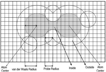
PB solvation model involves explicit representation of solute in a cavity with atomic coordinates including the corresponding atomic radii and partial charges on each atom. The solute is placed in a cavity of low dielectric constant embedded in a continuum solvent of high dielectric constant. The solute and the solvent boundary are obtained by rolling the probe of the size of solvent over the van der Waals surface as shown in figure 8. The electrostatic potentials are then calculated with PB equation using iterative procedures for quick solutions.
41
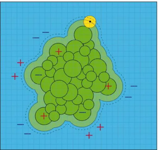
Figure 8: Schematic representation of the Poisson Boltzmann model of a molecule. The atoms in the molecule are represented by green spheres with partial charges and van der Waals radii. The high dielectric constant solvent is depicted in blue. The PB equation is solved on a three dimensional grid depicted in gray. The black line contour is obtained by rolling sphere with radius of water molecule shown in yellow on the van der Waals surface of the molecule. The boundary of ion-accessible volume is denoted by dashed line contour.66
The higher dielectric constant of the solvent in the PBE equation includes the induced, permanent dipoles and the orientation of the solvent around the solute. The dielectric constant of the solute, mainly in case of protein, has lower dielectric constant in the range of ε ~ 2-20. Its value varies depending on the type of protein and the simulation method used in PBE model. The lower dielectric constant value, ε = 2, is used if only electronic polarizability of the protein is considered where as higher value (~ 20) can be used to account for the polarizability and charges reorganization.67, 68 The dielectric constant of solute particularly in case of protein is a
42
nontransferable parameter. It is required to calculate the electrostatic interactions such as charge-charge interactions or charge-charge-solvation which depends on the shape and the exact location of the charges in the solute. The accuracy of the biomolecular applications require separate parameterization of macromolecule dielectric constant depending on the applications used.
PB model is a physically simple method to compute the electrostatic component but its numerical solutions for complex shapes and charge distributions are associated with high computational cost and do not scale well with increase in the size of the system. Typically, this differential integral equation is solved using finite-difference method (FDM) 69 in molecular mechanics simulations. In this method, molecular charges and dielectric are discretized on the grid and the Poisson-Boltzmann equation is solved and recast in a finite difference form. There are several problems associated with the discretization procedure such as the grid must be fine enough to represent accurately solute-solvent interactions and not merge opposite charges on the same node. Also, the free energy will depend on the grid spacing and the relative position of charges on the grid. Since the algorithms for solving Poisson-Boltzmann equation using finite difference methods is still computationally demanding many advancements such as multigrid methods are applied in biochemistry for faster simulations. Other methods that avoid the discretization problems are boundary element and finite element methods (FEM). The boundary element approach is less popular in molecular mechanics and is mostly applied in quantum calculations for small organic molecules.70
Although several methods have been devised to solve PB equation but it is still not feasible to solve it for molecular dynamics (MD) or Monte Carlo (MC) simulations where large
43
conformational sampling is required. The earliest attempts of wide applicability of PB equation to dynamic simulations demanded high computational effort and thus had limited scope. It was observed that simulation cost per-step with FD method even with 1-Å grid spacing was higher than with the explicit water simulation although the latter took longer time to equilibrate whereas with PB model, water is always equilibrated. This limits the practical applications of PB equation in MD simulations of biological molecules.
Though there is a continuous progress in numerical methods to solve PB equation but high computational effort and complexity in case of macromolecules has led to the development of approximations to the PB equation through methods such as Generalized Born (GB) model,71 Dielectric Screening model,72 Induced Multipole Solvent models73 and others. These approximate models are widely used to treat solvation but none of them model the solvation effects as accurately as the PB equation especially in case of desolvation of charged groups occurring often in protein dynamics.
The approximations to Poisson-Boltzmann equation such as Born equation and its modifications are used for more faster simulations of complex systems. The Born equation is the simplest case of calculating electrostatic solvation free energy of a charged ion from gas phase to the solution.
44
Born Equation
(Generalized Born (GB) model)
71Born Equation
Born equation illustrates the electrostatic free energy in transferring a spherical charged ion with radius α from a medium of dielectric constant εi to a medium of dielectric constant εo (Equation 17).
(17)
Born equation was first derived by setting the dielectric constant εi = 1 as in the case of vacuum.
Born equation can be used with Coulomb’s law to calculate the free energy change in moving a point charge between the two homogeneous media (Figure 9).
Figure 9: Schematic illustration of Born equation (ion). Spherical ion of radius α transferred from vacuum to water. The reaction field due to surface charges produced as a result of induced polarization in water stabilizes the ion.
Born equation is derived from classical electrostatics theory according to which the total electrostatic energy in the dielectric media is given by the equation (18) and equation (19)
(18)
(19)
45
E and D in the equation (18) and (19) represent the electric field and electric field displacement respectively. ε is the dielectric constant of the medium.
Gauss law is used to obtain E and D.
or
(20)
The left integral in the equation (20) depict the area integral over the surface whereas the right integral is the volume integrated over the whole space enclosed by the surface. Here n(r) represent the normal of the surface and ρ is the free charge density.
The electric field and electric displacement inside and outside of the uniformly charged spherical shell with dielectric εi inside and outside can be given
(21)
In the equation (21), q represents the total charge of the sphere and the center of the coordinate is set at the center of the sphere. The total electrostatic energy of the system can now be calculated using the above equations as
46
(22)
In the equation (22), α represents the radius of the sphere. Similarly, the total electrostatic energy for a system of uniformly charged sphere with dielectric constant inside and outside as εi
and εo respectively can be written as
(22)
The energy difference between the two systems is evaluated as Born equation.
However if there is more than one charge, an approximation to the Born equation known as Generalized Born Equation (GBE) is used.
Generalized Born (GB) model)
71The pairwise GB model is based on the same dielectric continuum solvent model as PBE. Generalized Born model have been widely used to calculate the ligand binding free energies, in conformational analysis of proteins and in drug designing. It is one of the most efficient approximations of the solution of Poisson-Boltzmann equation for a charge in the centre of an ideal spherical solute of radius α and dielectric constant εi for the interior and the ε0 for the
exterior solvent. This model is extension of Born model which evaluates the change in free energy in moving a point charge from vacuum to spherical cavity of the solvent.
47
The generalization of Born model to solutes of different cavity shape and simulating the solutes as a collection of small spheres of atoms of charges qi and radius αi or point charges placed in the
center of the spheres with the inner dielectric constant of the sphere as εi forms the GB
formalism.
The electrostatic interactions between the point charges are calculated as a sum of Coulomb interactions in vacuum and the self-energies of the spheres. The self-energy can be decomposed into the total electrostatic energy of spheres placed in medium with dielectric constant εi, and the
electrostatic solvation energy. In case of real solutes the Still and coworkers used pairwise sum over interacting point charges approximation to calculate solvent induced reaction field energy known as Generalized Born (GB) equation (Equation 24-26)
(24)
(25)
(26)
In equation (27) εi and ε0 are dielectric constant of interior and exterior medium, rij is the
distance between the atoms i and j, and αi is the generalized Born radius of atom i.
The estimation of effective Born solvation radius, αi, or the distance between charge and the
48
energy. This is adjustable parameter and can be calculated using solvation free energy from Poisson-Boltzmann equation or less expensive alternating methods. Although PB solvation model is the most accurate representation of continuum solvation, GB methods provide potentials for faster simulations of larger systems. GB models are also combined with the surface area and referred to as GBSA models to estimate the hydrophobic contributions to the solvation free energy as well. These models are particularly useful in many ligand docking programs.
Implicit Solvation Models based on solvent-accessible surface area
The continuum solvent accessible surface area (SASA) solvation models are based on assumption that interactions between the solute and the solvent are proportional to the surface area. It computes the nonpolar contribution of total free energy of solvation. This model was first parameterized by Eisenberg and McLachlan74 to compute free energy of transfer of amino acids between octanol and water. The solvent-accessible surface area as defined by Lee and Richards and others is the area moved by center of water molecule of radius 1.4Å around the group without any unobstructed contact with the group. The SASA based continuum model was also parameterized by Ooi75 et al to compute thermodynamic solvation parameters for seven classes of groups occurring in peptides by fitting to the experimental free energy of solvation of small aliphatic and aromatic molecules.
The non-electrostatic contributions to the total free energy of solvation are usually given as a linear function of the solvent-accessible surface area according to the equation (27)58(e), 61(d), 76
49
ΔGnp represents the nonpolar free energy and A is the solvent accessible surface area in the equation 27. The proportionality constant γ or the surface tension is the contribution to the solvation energy per unit surface area obtained by fitting to the experimental data. Another constant b represents the free energy of hydration for a point solute.
Although surface area models have worked well based on theoretical and experimental observations of transfer free energies of small chain alkanes from oil to water and vacuum to water in being related linearly to surface area, there are discrepancies in this model. Some of these include the wide range of surface tension proportionality constant corresponding to the definition of solute surface area77 (van der Waal, molecular or solvent accessible surface area), parameterization of the model to the different experimental data as well as the application of the model to small organic molecule solvation and complex molecules and binding.
On the careful analysis of nonpolar contribution to the solvation energy in case of small and complex molecules such as proteins, this has been decomposed into energy penalty for cavity formation due to excluded volume effects and van der Waal dispersion forces between the solute and solvent (Equation 28).57
(28)
It has also been shown that ΔGvdW or free energy change for establishing attractive interactions
between the solute and solvent for a set of alkanes of similar size is a function of the solute composition and not its surface area. This explains not only the small hydration energy of cyclic
50
alkanes in comparison to the linear alkanes but also the requirement of two surface tension parameters of alkanes to reproduce their hydration free energies and conformational equilibria.
The applications of these models have been limited due to the high cost of calculating accurate solvent accessible surface areas. Some of these limitations have been circumvented by approximating solvent accessible surface areas usi