Economic Impacts of the Conservation Reserve Program: A General Equilibrium Framework

Economic Impacts of the Conservation Reserve Program: A General Equilibrium Framework

Farzad Taheripour

Contact Information: Farzad Taheripour

Department of Agricultural and Consumer Economics University of Illinois at Urbana Champaign

402 Mumford Hall, MC-710 1301 West Gregory Drive

Urbana, IL, 61801 Tel: (217) 333-3417 Fax: (217) 333-5538 E-mail: [email protected]

Selected Paper prepared for presentation at the American Agricultural Economics Association Annul Meeting, Long Beach, California, July 23-26, 2006

Copyright 2006 by Farzad Taheripour. All rights reserved. Readers may make verbatim copies of this paper document for non-commercial purposes by any means, provided that this copyright notice appears on all such copies.

Economic Impacts of the Conservation Reserve Program: A General Equilibrium Framework

Abstract

This article uses a general equilibrium framework and econometric analyses to examine

economic wide impacts of the Conservation Reserves Program. It determines direct and indirect factors which affect the economic efficiency of the program and shows their magnitudes. It shows that the interaction between the program and the tax system causes indirect efficiency costs but the interaction between the program and the agricultural support subsidies generate economic gains. The program has the potential to distort the labor market and cause efficiency losses form this channel. However the analytical model shows that trade can reduce social costs of the policy because a part of the burden of the policy can be passed on to foreign consumers of crop products through the world market. The numerical results show that at the current level of acreage reduction (34 millions acres), the marginal cost of spending one more dollar on the program is about $1.9 for the US economy. In addition, the numerical results illustrate that the program has the potential to generate different and significant unintended economic impacts. For example, depending on the parameters of the model, the program can raise the prices of land up to 10.6%, generate up to 20% land conversion, and raise the demand for nitrogen fertilizer up to 4.2% at the current level of acreage reduction. Finally, the empirical regression results

demonstrate that the program has affected the production behavior of the crop industry

significantly. In particular, the program has increased the demand for fertilizer and labor and has decreased the demand for land and capital.

Keywords: land retirement, slippage effect, efficiency cost, agricultural pollution, tax system

Introduction

Acreage reduction programs have played a major role in the US agricultural policy in the past 73 years, at least from the passage of the Agricultural Adjustment Acts of 1933 and 1938 (Ericksen and Collins, 1985). Prior to 1986, acreage reduction programs have been mainly used to control and reduce crop production based on the short term contracts. The Conservation Title of the 1985 Food Security changed this pattern and allowed the government to retire environmentally

sensitive croplands based on the long term contracts (10 to 15 years). The Conservation Reserve Program (CRP), which has been established under this act, has begun retiring cropland in 1986. This program has retired about 34 million acres of cropland shortly after its beginning and continued to set aside the same acres of cropland from production thereafter1.

Figure 1 shows the history of retired acres during 1955 to 2004. This figure shows that unlike other acreage reduction programs, which retired land with a high degree of dispersion over time, the CRP has persistently retired about 34 million acres of land during its presence. This program which extensively targets land use in agriculture over time has the potential to affect resource allocation in the whole economy and particularly in agriculture. This paper aims to estimate the overall efficiency costs of this program regardless of its environmental impacts and examine its long term economic impacts on the demand for the main agricultural inputs including labor, land, capital, and fertilizer.

The economic efficiency of the acreage reduction programs and their economic and environmental consequences are important subjects that have been addressed frequently in the literature. The efficiency of alternative targeting instrument for selecting the land to be retired and the cost-effectiveness of retired acreages (in terms of forgone production and environmental gains) are two major issues that have been discussed extensively in the literature. Many papers

1 _{Retired acres under other acreage reduction programs (such as the Soil Bank Program and the Acreage Reduction}

Program) were returned to crop production during the period of 1986-1995. 3

investigate determinants of the cost effectiveness of land retirement and provide estimates of their magnitudes. For example, three recent papers in this field are Feng el al. (2005); Kirwan, Lubowski, and Roberts (2005); and Yang, Khanna and Farnsworth (2005).

In this field some papers demonstrate that the acreage reduction programs, in particular the CRP, have some unintended impacts which may reduce their efficiency (For example see Hoang, Babcock, and Foster (1993) and Wu 2000)). They mainly address the slippage effects of land retirement. Slippage effects arise for two main reasons: an increase in the use of non-land inputs and the diversion of less productive land to crop production. For example, Wu (2000) shows that for each one hundred acres of cropland retired under the CRP twenty acres of non-cropland were converted to non-cropland in the central United States. In a recent article Roberts and Bucholtz (2005) question the reliability of Wu’s empirical findings. However, their work provides an evidence for the land conversion (Wu, 2005)

Previous papers which study economic impacts of the acreage reduction programs typically apply partial equilibrium frameworks in their analyses and ignore general equilibrium impacts of these programs. The CRP is a large program that can affect the whole economy from different directions. The government finances this program from the distortionary income taxes ($1.8 billion per year). This can adversely affect the economic efficiency through the tax system. This program has the potential to affect prices of agricultural inputs and outputs and affect the farmers’ behavior. For example, when nitrogen and land are substitute inputs, the CRP can encourage farmers to apply more nitrogen (and other inputs). An increase in applied nitrogen may adversely affect the water quality which in turn imposes indirect cost on the economy. In addition, more demand for non-land inputs (such as fertilizer, capital, and labor) restricts

resources available in production of other goods and services which in turn reduces welfare. The CRP has the potential to raise prices, in particular prices of crop products, which consequently

reduces welfare of consumers. The CRP may also reduce incentives to work and raise inefficiency in labor market.

The CRP has positive and welfare improving impacts as well. It raises prices of crop products and therefore reduces the need for the commodity price support subsidies. This can generate economic gains through the tax system. Furthermore, since the US is a large exporter of crop products, the CRP can raise the prices of these commodities in the world market (Sumner, 2003). This can generate economic gains for the US economy. In addition to these economic benefits, the CRP reduces soil erosion, provides wildlife habitat, and improves water quality.

This paper investigates long run economic impacts of the CRP program at a macro level for the US economy regardless of its environmental consequences. It first examines the

economy-wide impacts of the program by developing a stylized analytical and numerical general equilibrium model. The general equilibrium model is built on the theory of environmental regulation in the second best setting setting2. In particular, the model is an extension of Taheripour, Khanna, and Nelson (2006). The model first examines unintended impacts of the CRP and their determinants and then measures their magnitudes. Finally, the paper applies an econometric analysis to seek empirical evidence for unintended impacts and study impacts of the program on the demand for the main agricultural inputs at a macro level. The econometric analysis follows Ray (1988) and sheds light on the impacts of the CRP on the economic parameters associated with the crop production at an aggregate level.

Section 2 presents the analytical general equilibrium model and determines factors that affect efficiency costs of an incremental increase in retired land. Section 3 describes the numerical model and calibration process. Section 4 contains results of the numerical model. Section 5 demonstrates the regression analysis followed by the conclusion in Section 6.

2 _{Throughout this article, the term “second best” refers to a setting with prior distortionary income and commodity}

taxes/subsidies.

The Analytical Model

Consider an open economy with one representative consumer, two producers, and a regulator. Each producer produces only one final good. Hence, there are two final goods: X and Y. Here X represents a homogeneous crop product and Y stands for other goods and services. Output of these goods and their prices are indicated with OX, OY, , and , respectively. The resources

used in production of both goods are labor, land, and capital. Endowments of these resources are

X

p p_Y

L,R, andK_{, and they are fixed. Land and capital are fully employed. However, the}

consumer consumes some part of the labor endowment as leisure, l. The wage rate, w, is selected as the numeraire. Prices of land and capital are and . The crop producer uses nitrogen fertilizer in its production process as well. The economy imports nitrogen fertilizer, , at a constant price R r r_K X N 3 _of N

p and exports some part of its crop product, x, at the price of . Domestic markets are all competitive and agents are price takers. We assume free trade with no tariffs. The demand for exports,

X

p

( _X)

x p , is downward sloping, with a constant price elasticity of ε_x. The balance of trade, Z, can be positive or negative and is defined as follows:

(1) (Z = p x p_{X X} )+ p N_{N X}

The consumer derives utility from consumption of goods, leisure, and foreign reserves. The utility function is given by:

(2) (U =u C C l_X , _Y , )+ϕ( )Z .

Here CXand CY show domestic consumption of X and Y, respectively. In the utility function

l = −L Lis leisure and L is labor supply. We assume that u(.) is increasing in all arguments and is quasi-concave and that ϕ( )Z is increasing in Z and weakly concave. The representative consumer takes Z as given. We consider reserves as an opportunity to import other goods from

3 _{We will incorporate the elasticity of supply of nitrogen in the world market in the numerical model.}

the world market. Alternatively, we can interpret reserves as a public asset/debt. The consumer supplies labor, land, and capital and receives a lump sum transfer, G, from the government. The consumer budget constraint is:

(3) (1p C_{X X} +p C_{Y Y} = −t L Q_L) + .

Where Q = −(1 t r RR) R + −(1 tK)r KK −Z +G represents consumer’s non-labor incomes.

Here , , and are flat tax rates on labor, land, and capital incomes. The following demands for goods, supply of labor and indirect utility function, V, can be derived from utility

maximization: L t t_R t_K (4) C_X =X p( _X ,p_Y ,(1−t_L), )Q , (5) C_Y =Y p( _X ,p_Y ,(1−t_L), )Q , (6) L =L p( _X ,p_Y ,(1−t_L), )Q , (7) (V =v p_X ,p_Y ,(1−t_L), )Q +ϕ( )Z .

Production functions represent constant returns to scale (CRS) and are represented by: (8) O_X =X L( _X ,R_X ,K_X ,N_X ),

Y

X

(9) O_Y =Y L R K( _Y , _Y , ).

Since production functions exhibit CRS, the marginal and average cost functions are equal to each other. In addition, because markets are competitive, prices of goods equal marginal costs in the absence of price support subsidies. These assumptions imply:

(10) ( ,MC_X =MC_X r r p_{R K}, _N )= p , (11) ( , )MC_Y =MC r r_{Y K R} = p_Y .

Here, MCX and MCY represent marginal costs of X and Y, respectively. Competitive markets and

CRS technologies impose zero profits in both sectors. In equilibrium, the supply of X must equal its domestic demand plus exports and the supply of Y must equal its domestic price. That is:

(12) (O_X =C_X +x p_X ), (13) O_Y =C_Y .

Furthermore, market clearing conditions for the primary inputs and nitrogen should be satisfied. In this economy, the government has several functions. It supports crop production gh a subsid er unit of output, So, and retires land, RG, to protect environment. The

govern

st

throu y p

government also taxes incomes and pays a lump-sum transfer, G, to the consumer. The ment is committed to a certain level of real lump-sum transfer. Therefore, it adjusts G with changes in the prices of consumption goods. In equilibrium government revenues mu equal government expenditures. That is:

(14) t L N_L + _LTR =S X_o +r R_{R G} +G ,

here N_LTR =t r R t r K_{R R} + _{K K} and N_LTR stands for non-labor tax revenues. Since the governm supports production of crop through a subsidy per un

ent it of output, the consumer price of each unit s:

X X R K o

of X i

(15) p =MC ( ,r r p, _N ) .

CPF) from the labor tax as: S

−

To express results succinctly, we define the partial equilibrium marginal costs of public funds (M ( / ) /( ( / )) L L L L M = − ∂t L ∂t L t+ ∂L ∂t (1 ) MCPF = = +τ M , where (16) We als ) L L

o define the partial equilibrium marginal excess burden (MEB) of the labor tax as:

(17) ( C / ) /(

L L

MEB =τ′= −t ∂L ∂t L +t (∂L/∂t ) .

superscript C indicates c ted derivative of labor supply with respect to the labor tax. labor y elasticities. We define elasticity of labor supply with respect to non-labor income

Here ompensa

These measures are basically distinguishing between the compensated and uncompensated suppl

byεLQ =(dL dQ Q L/ )( / ). Following the literature we assume thatεLQ <0. We denote the share

of lump-sum transfer in total income as: (18) /((1S =G −t L Q) + ).

Fin

G L

ally, we defineλas the

lfare impacts of an incremental increase in RG we first

y differentiate the utility function with respect to this variable. Then we define components ions (1) through (15) to trace welfare

(19)

consumer’s marginal utility of income. To examine direct and indirect we

totall

of this equation through different steps. In these steps we use equat

impacts of the policy from all markets. In this process we apply definitions (16) through (18), the Slutsky equation, and Shepard’s lemma to shrink the final result into compact

components4. Note that in this derivation, it is assumed that tR and tK are constant. Equation (19)

shows the final result, where each positive component represents a positive change in the welfare and vice versa.

Pr Re Pr 1 ( ) (1 ) ( 1) ( 1 X G X G G G G

imary tirment Effect imary Trade Effect

dp du X dX d dZ dx p S ε x ϕ p ⎛ ∂ ⎞ ⎛ ⎞ = −_⎜ − − _⎟ +_⎜ − + − − _⎟ ) ( ) X o x X R LTR R G o G G G dR R dR dR dZ dR dR dr dN dX r R S dR dR dR λ λ τ ∂ ⋅ ⎝ ⎠ ⎛ ⎞ ⎛ ⎞ − _⎜ + _{⎟ ⎜}− + − _⎟ ⎝ ⎠ ⎝ ⎠ ⎝ ⎠ − 1444442444443 144444444424444444443 ( ) Re Re Re , (1 ) (1 )

verse venue cycling Effect

R K

L LQ R K

N N N

Non Labor Income Effect

J L J G J X Y J G L dr dr L dZ t R t K t Q dt dt dt dp L t C s p dR τ ε τ τ − = ⎛ ⎞ ⎜ ⎟ ⎜ ⎟ ⎝ ⎠ ⎛ ⎞ ⎛ ⎞ + _{⎜ ⎟⎜} − + − − _⎟ ⎝ ⎠ ⎝ ⎠ ⎛ ⎛ ∂ ⎞ _′ ⎞ − ⎜_⎜ ⎜−_∂ ⎟+ ⎟_⎟ ⎝ ⎠ ⎝ ⎠

∑

14444444244444443

The first component which is labeled primary retirement effect is equal to the value of marginal product of land minus total saving in agricultural subsidies due to the reduction in X.

4 _{Detailed derivation is available from the author on request.} 9

This is

e ugh the trade channel. The first subcomponent of the trade effect measures changes in the exp

the opportunity cost of retired land regardless of other impacts of the policy on the economy.

The second component which is labeled primary trade effect measures impacts of th policy thro

ort value of crop product due to an increase inR_G. An increase in retired land has the potential to restrict supply of crop product. Therefore, when the price elasticity of demand for crop product in the world market,ε_x,is less than one this term is positive. In this case an incre in _G

ase R decreases export volume of crop product but increases its export value. The second

subcomponent of the trade effect m sures changes in the utility of reserves due to an increase in

ea

G

R . The sign of this effect depends on two terms: dZ dR_G and d dZ

ϕ

λ . The first term shows direction of change in the reserves due to an increase inR_G and the second term represents the

the marginal utility of reserves over the marginal utility of income. An increase in retired ratio of

land may either increase or decrease the reserves. When land and nitrogen fertilizer are complement, an increase in RG would reduce the demand for nitrogen which in turn raises the

reserves, recall thatε_x <1. However, when these two inputs are substitutable then and in in R

crease s.

G would increase the demand for nitrogen fertilizer which can lead to a reduction in reserve

The econometric results presented below and previous work in this field indicate that at a macro level land and nitrogen are substitutable (for example see Hertel, Stiegert, and Vroomen 1996). In the rest of this section we assume that land and nitrogen are substitutable. We now turn to the term d

dZ

ϕ λ

term is equal to one and as the result the second subcomponent of the trade effect will be

vanished. However, when these marginal values are different then the second component will be . When the marginal utility of reserves is equal to the marginal utility of income this

materialized. One can expect d 1 dZ

ϕ

λ > when the economy is faced with a trade deficit and

1 d dZ ϕ λ tive arginal va

< when there exist a trade surplus. In conclusion, the second subcomponent is posi

and welfare improving when the m lue of reserves is larger enough and 0

G

dR . dZ _>

Finally, the last subcomponent of the trade effect measures an increase in utility due to diverted exports to domestic consumption. In inclusion, whenε_x ≤1, dϕ/dZ is large enough, and

0

G

dZ dR > the trade effect offsets some part of the primary retirement costs.

The third component which is labeled reverserevenue recycling effect is a welfare reducing item and measures efficiency costs of additional labor tax that is needed to finance the policy. This effect is equal to the marginal cost of public funds minus one times the net change in government expenditures due to an increase in RG. In one hand the government raises the labor

tax rate to pay rental value of re

G

es consumers’ income from these resources and discourages labor supply.

tired acres to their owners. This imposes some efficiency costs to the economy. On the other hand the policy raises the non-labor tax revenues, mainly due to an increase in the price of land. In addition, as mentioned earlier, the policy reduces the needs for agricultural subsidies. These two items eliminate some burdens of labor tax that is needed to finance the policy.

The fourth component which is labeled non-labor income effect reflects the impacts of the policy on the labor supply due to changes in the consumer’s non-labor income. The non-labor income effect is a negative and welfare reducing item as well. An increase in R elevates the prices of land and capital which accordingly rais

Finally, the fifth component which is labeled land retirement and labor tax interaction effect reflecting the efficiency costs due to interaction between changes in the prices of goods

and the labor tax rate. An increase in RG increases prices of both goods which in turns reduces

the real wage and discourages labor supply. The interaction effect captures the efficiency costs of

reducti n

es several

directions. This section develops a numerical model to measure the overall efficiency rtions of acres and gauge their corresponding impacts on the economy.

the

(20)

on in real wage. This effect has two major subcomponents. The first subcomponent (whe J=X) is the interaction effect due to changes in the price of crop products. The second

subcomponent (when J=Y) is the tax interaction effect due to changes in the price of the other good.

The Numerical Model

The above analytical analysis shows that an incremental increase in retired acres impos primary and secondary efficiency costs to the economy and it affects economic variables in several

costs of retiring large po

The numerical model follows the analytical model and depicts the US economy at a macro level. The representative consumer derives utility from goods and leisure according to following two-level constant elasticity of substitution utility function:

( )

(

)

(

)

In this utility functionρ_U =(σ_U −1) /σ_U , (ρ_C = σ_C −1) /σ_C, σ_uis the elasticity of substitution between leisure and consumption goods, σ_Cis the elasticity of substitution between the two

ption goods,

consum α_land α_Xare distribution parameters andϕindicates marginal utility of the reserve.

We model production processes with two-level production functions introduced by Sato d e

nd convenient way to build up constant elasticity of substitution (CES) production (1967) and widely used in literature (for example see Binswanger 1974; Kawagoe, Otsuka, an Hayami 1985; Thirtle 1985; Abler and Shortle 1992). This typ of production function provides a simple a

functio

(21)

ns with more than two factors of production. In a two-level production function, first, production is a function of two composite inputs: which are called mechanical and biological inputs. Second, production of each composite input is a function of two inputs. The biological input is a function of land and fertilizer and the mechanical input is a function of capital and labor. The production functions are written as:

{

}

i ii ii i ii

O ₌

γ α

α

(22)

{

}

(1

)

B

₌

γ

α

R

_{+ −}

α

N

{

}

i

i Mi Mi i Mi

M ₌ γ α Lρ _{+ −}α Kρ ρ

(23) , for i=X and Y.

Here Oi, Bi, andMirepresent outputs of final goods, composite biological inputs, and

anical inputs, respectively. In these product ctio e distribution and adjustment parameters,

mech ion fun ns α’s and γ’s ar

( 1) /

ii ii ii

ρ = σ − σ , (ρ_Bi = σ_Bi −1) /σ_Bi,ρ_Mi =(σ_Mi −1) /σ_Mi , and σ_iiare

the elasticities of substitution between the biological and the mechanical inputs,σ_Biare the elasticities of substitution between land and nitrogen andσ_Miare the elasticities of substitution between labor and capital. It is assumed that production of does not need nitrogen. This implies that

Y

1

BY

α

=

Data

rk data, so parameters are taken from the literature. The pensated labor supply elasticity of

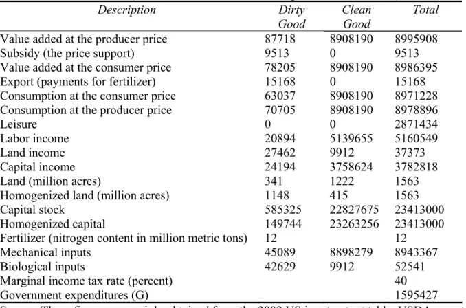
Table 1 depicts the US economy in 2002. In this table, the US economy is divided into two sectors: a sector which produces crop products and a sector which provides other goods and services. In addition to the benchma me

uncom e_L =0.15 is taken from Goulder et al. (1999). The

price elasticity of 1.0is assigned to the demand of the clean good based on the work of

Y

p

e =

Kyer and Maggs (1997). Their work indicates that the price elasticity of aggregate demand f the US economy was around 1.0 during the time period of 1965-90. This value is adopted because the clean good approximately represents an aggregate demand for the US economy. Based on the Database for Trade Liberaliz dies (Sullivan et al. 1989), the price elastic of ep_X =0.5 is assigned to the domestic demand of the dirty good. This number represents an inelastic demand for crop products. Furthermore, we assume that the elasticity of demand for crop products in the world market is equal to _x 0.9

or

ation Stu ity

ε = . These elasticities are used to calibra parameters of the utility function. To incorporate the supply of nitrogen into the model, it is assumed that the supply of nitrogen is increasing in its price. To measure sensitivity of results to the price elasticity of supply of the nitrogen, the model is solved for three different values of th elasticity. The selected elasticities are: (ε

te

is f

(1996). They are shown in table 2. We also do sensitivity analyses to

Efficiency Costs and Unintended Impacts

EV 5

0 1

ctions,

SN = 0.5, εSN = 1.0, and εSN = ∞). Finally, elasticities o substitution in the production functions are ta Balisteri et al. (2002) and Horan et al.

check how results change due to changes in the selected parameters.

To evaluate the efficiency costs an equivalent variation measure ( ) with the following extended definition is calculated for each target of acreage withdrawal:

(24) , and .

Here ( , )e and ( , )v stand for the expenditure and indirect utility fun ken from

(2002), and Hertel et al.

0 0 0 1

( , ) ( , )

EV =e p u −e p u _u0 _{=v p m(} 0_{, ) u}1 _{=v p m( ,}1 ₎

0

p and _p1_represent

n the absence and presence of land retirement, and this . This definition

vectors of prices (including prices of inputs) i

0

m and _m1 _{indicate wealth in the absence and presence of land retirement, respectively. In}

definition, wealth includes all types of income, leisure, and trade reserves

5 _{This definition is designed based on the question 3.I.12 of Mas-Collel, Whinston, and Green} (1995).

captures changes in both the prices and wealth. In this definition, a positive amount of EV ents w re los

6

Effic y c

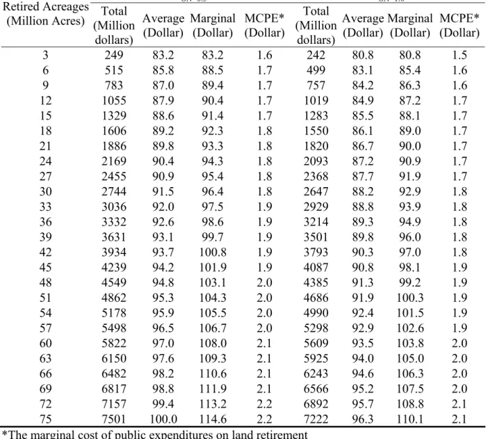
Results for three values of the elasticities of supply of nitrogen fertilizer (ε = 0.5, ε = 1.0, and

ε = ∞) have been reported in table 3. Four figures for each of these elasticities have been presented in this table: total, average, and marginal costs for each level of acreage reduction and the marginal cost of public expenditures (MCPE) associated with that level. The total costs gauge reduction in welfare in terms of EV due to the designated level of land retirement. The average costs show welfare lost per acre of the retired land and the marginal costs represent welfare lost of the last units of the retired land. Finally, the last figures, MCPE, compare the marginal costs with the amount paid per acre of the retired land by the government in 2002. The MCPE measure the unaccounted social costs of government land retirement payments.

Table 3 shows that for each level of the retired land, costs are decreasing in the elasticity of supply of nitrogen fertilizer. For example, the first acre of the retired land costs the economy $83.2, $80.8, and $74.3 when ε = 0.5, ε = 1.0, and ε = ∞, respectively. In the rest of this section we focus on the results for the unit elasticity of nitrogen supply, ε = 1.0, to be neutral with respect to this parameter.

Table 3 illustrates that costs grow with the level of acreage reduction. For example, the first and the last retired acres cost the economy $80.8 and $110.1. These figures are 1.5 and 2.1 times of the money that the government has paid for each acre of retired land in 2002. The

repres elfa s. The numerical model is calibrated and then solved for several consecutive targets of acreage reduction (from 3 to 75 million acres) using Mathematica.

ienc osts

SN SN

SN

SN SN SN

SN

6 _{To evaluate the precision of the calibration process and measure the simulation capability of the} calibrated model, the status quo is simulated first. The simulation of the status quo shows negligible differences (usually less than one percent) between real data and their simulation figures.

federal government has paid about $1.7 billion to withdraw 33 million acres of land from production, approximately $52 per acre of land.

9

ment CRP vernment decides to retire more land (for exampl

ucts

y of supply of nitrogen fertilizer. hat when the supply of nitrogen is more inelastic, land retirement generates

∞) are Table 3 reveals that the total social costs of retiring 33 million acres of land is about $2. billion for the US economy, about $88.8 per acre. The marginal cost of public expenditures for this level of land retirement is about $1.8. This means that the last dollar paid by the govern for the CRP program costs the economy $1.8. This umber reflects the marginal cost of the at the current level of acreage reduction. If the go

e to sequester carbon in the soil) costs will grow rapidly. For example, retiring 75 million acres of land (twice the current retired land) will cost the economy $7.2 billion, about $96.3 per acre. At this level of land retirement the MCPE will be $2.1

Unintended impacts

Numerical results reveal that land retirement largely affects the prices of land and crop prod and it has minor and negligible impacts (but positive) on the prices of capital and other goods. Table 4 shows impacts of acreage reduction on the prices of land and the price of the

homogeneous crop product for the three values of the elasticit This table illustrates t

stronger price impacts. For example, when the supply of nitrogen is very inelastic (εSN = 0.5), retiring 33 million acres of land raises the prices of land and the crop product by 10.6% and 4.1%, respectively. Corresponding figures for a perfect elastic supply of nitrogen (εSN = 9.3% and 3.3%, respectively. Furthermore, a careful review of table 4 reveals that the price impacts (change in the price of land and crop products) of land retirement grow exponentially with the amount of retired acres.

The price impacts of land retirement have the potential to affect both consumers and producers behaviors. In one hand, an increase in the price of land forces crop producers to apply

more labor, capital, and nitrogen fertilizer per unit of output. On the other hand, an increase the price of crop products encourages consumers to reduce their demand for crop products whi in turn forces farmers to reduce su

in ch pply of crop products. In the rest of this section we examine the imp

perfect

ith the

op

ber is very close to the reported figure by Wu, 2000). Table 5 shows that the size of

acts of land retirement on the demand for inputs and supply of crop products. Table 5 illustrates some of these effects for the three values of the elasticities of supply of nitrogen.

Table 5 illustrates that the aggregate demand for nitrogen fertilizer grows with the quantity of retired acreages. As explained earlier land retirement significantly raises the price of land compare to the prices of other inputs. This encourages crop producers to apply more nitrogen per unit of output. This eventually leads to an increase in the aggregate demand for nitrogen fertilizer. For example, table 5 shows that when the supply of nitrogen fertilizer is

ly elastic (εSN = ∞), retiring 33 million acres of land raises the aggregate demand for nitrogen fertilizer by 4.2%. The corresponding figure for an inelastic supply of nitrogen fertilizer (εSN = 0.5) is equal to 1.5%.Notice that applied labor and capital per unit of output grow w level of acreage reduction but their aggregate demand fall slightly due to the reduction in the crop production.

Table 5 illustrates that land retirement has the potential to transfer non-cropland to cr production. For example, when the supply of nitrogen fertilizer is very elastic, retiring 33 million acres of land generates a land slippage effect of 18.9%. This means that at this size of acreage reduction, for each 100 acres retired, about 18.9 acres of non-cropland would be converted to cropland (this num

slippage effect increases with the amount of retired acres and decreases with the elasticity of supply of nitrogen fertilizer. However, these factors do not affect the size of the land slippage effect very much.

Table 5 also shows that land retirement has a relatively weak impact on the crop

production. For example, when the supply of nitrogen fertilizer is very elastic, retiring 33 million acres of land reduces the supply of crop products by 1.8%. The corresponding figure for a

perfectly inelastic supply of nitrogen is about 2.3%. This means that land retirement restricts the

supply it of

icity of land and nitrogen fertilizer in production of the dirty good is reduced from

es of crop products moderately. This is because of using more non-land inputs per un output in crop production and because of the existence of the land slippage effect.

Sensitivity Analysis

To test impacts of alternative parameterizations on the simulation results, three more sets of parameters are tested. In the first set, the elasticity of labor supply is reduced from 0.15 to 0.11. This affects calibrated parameters of the utility function. In the second set, the elast

substitution between

1.25 to 0.75. This affects the calibrated parameters in sector X. In the third set, two more valu for the elasticity of demand for exports of the crop product,ε_x =1andε_x =1.1, are tested.

In short, a reduction in the elasticity of labor supply (from 0.15 to 0.11) reduces the efficiency costs but not significantly. A reduction in the elasticity of substitution between land and nitrogen fertilizer (from 1.25 to 0.75) makes substitution between nitrogen and land difficult and raises the efficiency costs and generates more slippage effect. Finally, results are slightly

sensitiv w

odel consistent with the rest of this paper roduction at the macro level is a function of four inputs: labor, land, e to the elasticity of demand for exports of the crop product. The efficiency costs gro with higher elasticities of demand for exports.

Econometric Analysis

This section applies regression analyses to explore impacts of the CRP on the demand for agricultural inputs and investigates structural change in the production parameters in the crop industry due to the CRP. To develop an econometric m

it is assumed that crop p

capital, and fertilizer (including all chemical inputs). Then it is assumed that the crop indus minimizes costs of production. Under these assumptions the structure of the production functio can be studied empirically using a cost function. A useful and flexible functional form that has been frequently used in defining cost functions is the translog form. For example, Ray (1982) estimated a two-output-five-input translog cost function for the US agricultural industry for the period of 1939-77. The translog cost function of Ray (1982) is modified in the current paper to study the US crop industry in the period of 1984-2004. According to Ray (1982), the following one-output-four-input translog cost function along with the corresponding input share equations have been defined and used in the current paper:

try n has 2 1 ln ln (ln ) ln ln 2 1 2 i i Xi i ij i J i i J C =α +α X + γ X +

∑

∑

∑

∑

∑∑

Here C represents the annual cost of crop industry, X stands for annual crop production, D is a dummy variable that represents presence of the CRP, Si shows cost share of input i, Pi represents

price of input i, and T is an annual index of time. The full system (i.e. the cost function and the share equations jointly) is estimated under the following restrictions to impose homogeneity of

j

degree one in input prices: 1 i α =

∑

∑

∑

∑

∑

∑∑

Notice that in this systemγ =γ . Using these restrictions, the full system has been transferred . In the modified system the price of labor has been selected as the numeraire. The Zellner’s Seemingly Unrelated method has been applied to estimate the modified translog system.

to a modified translog system

Data

The following variables have been collected for the period of 1984-2004: C, index of crop production expenses; X, index of crop production; PL, index of wage rate paid by farmers; PN,

fertilizer (including chemicals) price index: PR, index of rental rate of land: PK, price index of

nputs. The cost share variables are calculated using the crop industry expenses on labor,

e

red acres radually returned to production during this period. For thi

t onotonic because it generates positive fitted share at every observation. Finally, the

si concave in input prices because its Hessian matrix is negative semi definite uction other i

land, capital, and fertilizer (including all chemicals). The data has been taken from the Agricultural Statistics reports (1984 to 2004).

The dummy variable associated with the CRP has been defined based on the net acreag reduction during the sample period. The CRP program began enrolling farmland in 1986. However, the net retired acres during the period of 1984-96 were negative, because reti under other acreage reduction programs were g

s reason, the value of the dummy variable is zero in the period of 1984-96 and is one thereafter.

Empirical Results

A cost function should satisfy homogeneity, monotonicity, and convexity conditions. The homogeneity constraints were imposed throughout the estimation process. The estimated cos function is m

cost function is qua

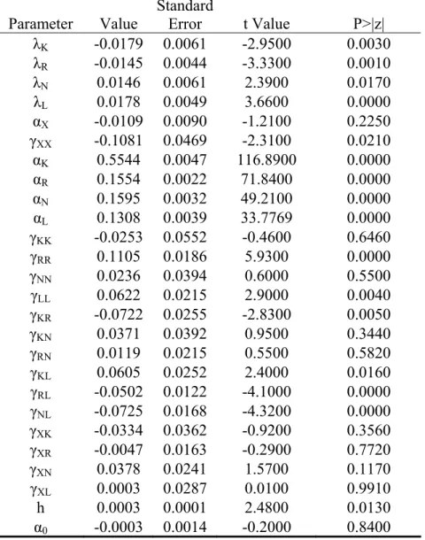
at every observation. Therefore, the estimated cost function represents a well behaved prod function. The Durbin-Watson test is preformed for each equation of the full system to test for autocorrelation. There was no sign of autocorrelation. The estimated parameters are reported in table 6. This table indicates that those parameters which demonstrate structural change in the cost and share equations (i.e.λ_K, λ_R , λ_N , andλ_L) are all statistically significant (at least at 5%

level of significance). The signs of these parameters show that the CRP has had negative impacts on the demands for capital and land and positive impacts on the demands for nitrogen and labo

It is straightforward to eri s ifican conomic parameters such as elasticities of substitutions between inputs and the price elasticities from the estimated cost function parameters. The Allen partial elasticity of substitution is frequently used in the literature to

r. d ve ign t e

determine whether pairs of inputs are substitutes or complements. In a translog cost function, the Allen partial elasticities of substitution between inputs i and j, A

ij

σ , can be obtained from following formula: the ˆ ˆ ˆ ˆ ˆ ij i j ij i j S S S S γ + When A 0 ij σ > inputs A σ = ,

j and i are net substitutes and when A 0

ij

σ < they are net complements. Note that A A

ij ji

σ =σ , this means the Allen elasticity of substitution has symmetry attribute. In a translog cost function the own and cross price elasticities of demands for inputs also can be derived from

owing

the foll formulas, respectively: ˆ ˆ_{( 1)} i i S ε = ˆ − , ˆ ii i i S S γ + ˆ ˆ ˆ_{ij i j} ij S S γ ε = + . ˆ i S

Here ε_iJrepresent the cross price elasticity of demand for input i with respect to the price of input j and ε_ii stands for the own price elasticity of demand for input i. The scale economy is another significant economic parameter that can be derived from the estimated cost function

ete e

param rs. Following Christensen and Green (1976) the scale economy is calculated from th following formula:

1 ln / ln SEC = − ∂ C ∂ X .

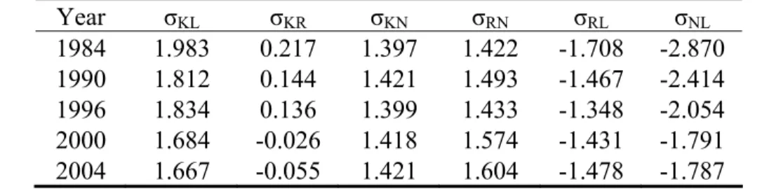
The pairwise Allen elasticities of substitution are computed and reported in table 7 for selected years. The table indicates that capital and labor; capital and nitrogen; and land and nitrogen were substitute during the sample period. Table 7 shows that capital and land were

substitu e le lar ctuating around (in of he icant rnment expenditure and causes s through the tax system. In addition, it acts as an implicit tax which reduces

e te at the beginning of the period but they became compliment at the end of period. Tabl 7 also indicates that land and labor and nitrogen and labor were compliment during the samp period. In general, elasticities of substitution have changed over the sample period, in particu after 1996. This confirms a structural change in crop production due to the CRP.

The computed own price elasticities are reported in table 8 for the selected years. This table shows that demand for inputs were relatively inelastic with respect to their own prices during the sample period. The own price elasticities of capital and nitrogen were flu

- 0.5 and -0.69, respectively. The own price elasticity of land has drastically decreased absolute terms) from -.17 to -.02 over the sample period. In contrast, the own price elasticity labor has significantly increased (in absolute terms) from -0.33 to -0.46 in the same period. T computed values of the scale economy are also reported in table 8 for the selected years. These figures were very close to 1 during the sample period. Finally, the computed cross price

elasticities are reported in table 9 for the selected years. This sign of these elasticities are consistent with the signs of elasticities of substitutions.

Conclusion

The CRP program which extensively and consistently retires cropland can generate signif direct and indirect economic consequences. It raises gove

efficiency cost

consumers’ real income and generates welfare losses. Since the program has the potential to rais the prices of crop products in the world market it may generate some gains from the trade

channel. At the current level of land retirement the program costs the US economy around $ billion dollars. The cost of program can grow exponentially if the government decided to retire more cropland. For example, retiring 75 million acres of cropland may cost the economy u $7.5 billion. The program has the potential to affect the demand for agricultural inputs, in particular demand for nitrogen and generate considerable amount of land conversion. The econometric results confirm these effects.

2.9

p to

Table 1. Benchmark Data (in millions of 2002 dollars except as otherwise noted) Description Dirty

Good Clean Good Total

Value added at the producer price 87718 8908190 8995908

Subsidy (the price support) 9513 0 9513

Value added at the consumer price 78205 8908190 8986395

Export (payments for fertilizer) 15168 0 15168

Consumption at the consumer price 63037 8908190 8971228 Consumption at the producer price 70705 8908190 8978896

Leisure 0 0 2871434

Labor income 20894 5139655 5160549

Land income 27462 9912 37373

Capital income 24194 3758624 3782818

Land (million acres) 341 1222 1563

Homogenized land (million acres) 1148 415 1563

Capital stock 585325 22827675 23413000

Homogenized capital 149744 23263256 23413000

Fertilizer (nitrogen content in million metric tons) 12 12

Mechanical inputs 45089 8898279 8943367

Biological inputs 42629 9912 52541

Marginal income tax rate (percent) 40

Government expenditures (G) 1595427

Source: These figures are mainly obtained from the 2002 US input output table, USDA reports, and the 2002 statistical abstract of the United States.

Table 2. Selected Parameters

Description of Parameter Value Source

Uncompensated labor supply elasticity 0.15 Goulder (1999)

Uncompensated price elasticity of demand for the dirty good

0.5 Steven et al. (2003) Uncompensated price elasticity of demand for the clean

good

1.0 Kyer and Maggs (1997)

Elasticity of substitution between the biological and the

mechanical inputs in production of X 0.5 Horan et al. (2002) Elasticity of substitution between land and nitrogen

fertilizer in production of X

1.25 Hertel et al. (1996) and Horan et al. (2002)

Elasticity of substitution between labor and capital in production of X

0.585 Balisteri et al. (2002)

Elasticity of substitution between the biological and the mechanical inputs in production of Y

0.5 Horan et al. (2002) Elasticity of substitution between labor and capital in

production of Y 0.951 Balisteri et al. (2002)

Table 3. Efficiency costs of acreage reduction for the US economy

εSN=0.5 εSN=1.0

Retired Acreages

(Million Acres) _(Million Total dollars) Average (Dollar) Marginal (Dollar) MCPE* (Dollar) Total (Million dollars) Average (Dollar) Marginal (Dollar) MCPE* (Dollar) 3 249 83.2 83.2 1.6 242 80.8 80.8 1.5 6 515 85.8 88.5 1.7 499 83.1 85.4 1.6 9 783 87.0 89.4 1.7 757 84.2 86.3 1.6 12 1055 87.9 90.4 1.7 1019 84.9 87.2 1.7 15 1329 88.6 91.4 1.7 1283 85.5 88.1 1.7 18 1606 89.2 92.3 1.8 1550 86.1 89.0 1.7 21 1886 89.8 93.3 1.8 1820 86.7 90.0 1.7 24 2169 90.4 94.3 1.8 2093 87.2 90.9 1.7 27 2455 90.9 95.4 1.8 2368 87.7 91.9 1.7 30 2744 91.5 96.4 1.8 2647 88.2 92.9 1.8 33 3036 92.0 97.5 1.9 2929 88.8 93.9 1.8 36 3332 92.6 98.6 1.9 3214 89.3 94.9 1.8 39 3631 93.1 99.7 1.9 3501 89.8 96.0 1.8 42 3934 93.7 100.8 1.9 3793 90.3 97.0 1.8 45 4239 94.2 101.9 1.9 4087 90.8 98.1 1.9 48 4549 94.8 103.1 2.0 4385 91.3 99.2 1.9 51 4862 95.3 104.3 2.0 4686 91.9 100.3 1.9 54 5178 95.9 105.5 2.0 4990 92.4 101.5 1.9 57 5498 96.5 106.7 2.0 5298 92.9 102.6 1.9 60 5822 97.0 108.0 2.1 5609 93.5 103.8 2.0 63 6150 97.6 109.3 2.1 5925 94.0 105.0 2.0 66 6482 98.2 110.6 2.1 6243 94.6 106.3 2.0 69 6817 98.8 111.9 2.1 6566 95.2 107.5 2.0 72 7157 99.4 113.2 2.2 6892 95.7 108.8 2.1 75 7501 100.0 114.6 2.2 7222 96.3 110.1 2.1

*The marginal cost of public expenditures on land retirement

Table 3. Continued

εSN=∞ Retired Acreages

(Million Acres) _(Million Total dollars) Average (Dollar) Marginal (Dollar) MCPE* (Dollar) 3 223 74.3 74.3 1.4 6 453 75.5 76.7 1.5 9 685 76.1 77.4 1.5 12 920 76.6 78.2 1.5 15 1157 77.1 78.9 1.5 18 1396 77.5 79.7 1.5 21 1637 78.0 80.5 1.5 24 1881 78.4 81.3 1.5 27 2128 78.8 82.1 1.6 30 2377 79.2 83.0 1.6 33 2628 79.6 83.8 1.6 36 2882 80.1 84.7 1.6 39 3139 80.5 85.6 1.6 42 3398 80.9 86.4 1.6 45 3660 81.3 87.4 1.7 48 3925 81.8 88.3 1.7 51 4193 82.2 89.2 1.7 54 4463 82.7 90.2 1.7 57 4737 83.1 91.1 1.7 60 5013 83.5 92.1 1.7 63 5292 84.0 93.1 1.8 66 5575 84.5 94.2 1.8 69 5860 84.9 95.2 1.8 72 6149 85.4 96.3 1.8 75 6441 85.9 97.3 1.8

*The marginal cost of public expenditures on land retirement

Table 4. Price impacts of acreage reduction (in percentage change compare to RG=0)

εSN=0.5 εSN=1.0 εSN=∞

Retired Acreages

(Million Acres) Price of Land Price of Crops Price of Land Price of Crops Price of Land Price of Crops 3 0.8 0.3 0.8 0.3 0.8 0.3 6 1.7 0.7 1.7 0.7 1.6 0.6 9 2.7 1.1 2.6 1.0 2.5 0.8 12 3.6 1.4 3.5 1.3 3.3 1.1 15 4.6 1.8 4.5 1.7 4.2 1.4 18 5.5 2.2 5.4 2.1 5.1 1.7 21 6.5 2.6 6.4 2.4 6.0 2.0 24 7.5 2.9 7.4 2.8 6.9 2.3 27 8.5 3.3 8.4 3.2 7.9 2.7 30 9.6 3.7 9.4 3.5 8.8 3.0 33 10.6 4.1 10.4 3.9 9.8 3.3 36 11.7 4.5 11.4 4.3 10.8 3.6 39 12.8 5.0 12.5 4.7 11.8 3.9 42 13.9 5.4 13.6 5.1 12.8 4.2 45 15.0 5.8 14.7 5.5 13.8 4.6 48 16.1 6.2 15.8 5.9 14.8 4.9 51 17.3 6.6 16.9 6.3 15.9 5.2 54 18.4 7.1 18.1 6.7 17.0 5.6 57 19.6 7.5 19.2 7.1 18.1 5.9 60 20.8 8.0 20.4 7.5 19.2 6.3 63 22.1 8.4 21.6 7.9 20.3 6.6 66 23.3 8.9 22.8 8.4 21.4 6.9 69 24.6 9.3 24.1 8.8 22.6 7.3 72 25.9 9.8 25.4 9.2 23.8 7.7 75 27.2 10.3 26.6 9.7 25.0 8.0 28

Table 5. Unintended impacts of acreage reduction (in percentage change compare to RG=0

except as otherwise noted)

εSN=0.5 εSN=1.0 εSN=∞

Retired Acreages

(Million Acres) Demand _for Nitrogen Land Slippage Effect† Supply of Crop Product Demand for Nitrogen Land Slippage Effect† Supply of Crop Product Demand for Nitrogen Land Slippage Effect† Supply of Crop Product 3 0.1 18.6 -0.2 0.2 18.3 -0.2 0.3 17.5 -0.2 6 0.2 19.5 -0.4 0.4 19.1 -0.4 0.7 18.2 -0.4 9 0.4 19.8 -0.6 0.6 19.4 -0.6 1.0 18.4 -0.5 12 0.5 19.9 -0.8 0.8 19.6 -0.8 1.4 18.5 -0.7 15 0.7 20.0 -1.0 1.0 19.7 -1.0 1.8 18.6 -0.8 18 0.8 20.1 -1.2 1.2 19.7 -1.2 2.2 18.7 -1.0 21 0.9 20.2 -1.4 1.4 19.8 -1.4 2.6 18.7 -1.2 24 1.1 20.2 -1.6 1.6 19.8 -1.6 3.0 18.8 -1.3 27 1.2 20.3 -1.9 1.8 19.9 -1.8 3.4 18.8 -1.5 30 1.4 20.3 -2.1 2.0 19.9 -2.0 3.8 18.8 -1.7 33 1.5 20.3 -2.3 2.2 19.9 -2.2 4.2 18.9 -1.8 36 1.7 20.3 -2.5 2.4 20.0 -2.3 4.6 18.9 -2.0 39 1.8 20.4 -2.7 2.6 20.0 -2.5 5.0 18.9 -2.2 42 1.9 20.4 -2.9 2.9 20.0 -2.7 5.5 18.9 -2.3 45 2.1 20.4 -3.1 3.1 20.0 -2.9 5.9 19.0 -2.5 48 2.2 20.4 -3.3 3.3 20.1 -3.1 6.3 19.0 -2.7 51 2.4 20.5 -3.5 3.5 20.1 -3.4 6.7 19.0 -2.8 54 2.6 20.5 -3.8 3.7 20.1 -3.6 7.2 19.0 -3.0 57 2.7 20.5 -4.0 4.0 20.1 -3.8 7.6 19.1 -3.2 60 2.9 20.5 -4.2 4.2 20.2 -4.0 8.1 19.1 -3.3 63 3.0 20.6 -4.4 4.4 20.2 -4.2 8.5 19.1 -3.5 66 3.2 20.6 -4.6 4.7 20.2 -4.4 9.0 19.1 -3.7 69 3.3 20.6 -4.8 4.9 20.2 -4.6 9.4 19.1 -3.9 72 3.5 20.6 -5.1 5.1 20.2 -4.8 9.9 19.2 -4.0 75 3.7 20.6 -5.3 5.4 20.3 -5.0 10.4 19.2 -4.2

† Converted acres from non-crop to crop production as a percent of retired acres.

Table 6. Estimated coefficients of the translog cost function Parameter Value Standard Error t Value P>|z|

λK -0.0179 0.0061 -2.9500 0.0030 λR -0.0145 0.0044 -3.3300 0.0010 λN 0.0146 0.0061 2.3900 0.0170 λL 0.0178 0.0049 3.6600 0.0000 αX -0.0109 0.0090 -1.2100 0.2250 γXX -0.1081 0.0469 -2.3100 0.0210 αK 0.5544 0.0047 116.8900 0.0000 αR 0.1554 0.0022 71.8400 0.0000 αN 0.1595 0.0032 49.2100 0.0000 αL 0.1308 0.0039 33.7769 0.0000 γKK -0.0253 0.0552 -0.4600 0.6460 γRR 0.1105 0.0186 5.9300 0.0000 γNN 0.0236 0.0394 0.6000 0.5500 γLL 0.0622 0.0215 2.9000 0.0040 γKR -0.0722 0.0255 -2.8300 0.0050 γKN 0.0371 0.0392 0.9500 0.3440 γRN 0.0119 0.0215 0.5500 0.5820 γKL 0.0605 0.0252 2.4000 0.0160 γRL -0.0502 0.0122 -4.1000 0.0000 γNL -0.0725 0.0168 -4.3200 0.0000 γXK -0.0334 0.0362 -0.9200 0.3560 γXR -0.0047 0.0163 -0.2900 0.7720 γXN 0.0378 0.0241 1.5700 0.1170 γXL 0.0003 0.0287 0.0100 0.9910 h 0.0003 0.0001 2.4800 0.0130 α0 -0.0003 0.0014 -0.2000 0.8400 30

Table 7. Allen elasticities of substitution between pairs of inputs (selected years) Year σKL σKR σKN σRN σRL σNL 1984 1.983 0.217 1.397 1.422 -1.708 -2.870 1990 1.812 0.144 1.421 1.493 -1.467 -2.414 1996 1.834 0.136 1.399 1.433 -1.348 -2.054 2000 1.684 -0.026 1.418 1.574 -1.431 -1.791 2004 1.667 -0.055 1.421 1.604 -1.478 -1.787

Table 8. Own price elasticities of demand for inputs and scale economies (elected years) Own Price Elasticities

Year εK εR εN εL Economies of Scale 1984 -0.49 -0.17 -0.69 -0.33 0.99 1990 -0.49 -0.12 -0.69 -0.40 1.00 1996 -0.52 -0.14 -0.69 -0.41 1.01 2000 -0.50 -0.01 -0.69 -0.45 1.02 2004 -0.49 0.02 -0.69 -0.46 1.02 Table 9. Cross price elasticities of demand for inputs (selected years)

Year εKL εLK εKR εRK εKN εNK εRL εLR εRN εNR εNL εLN 1984 0.22 1.10 0.04 0.12 0.24 0.77 -0.19 -0.28 0.24 0.24 -0.32 -0.48 1990 0.24 1.01 0.02 0.08 0.23 0.79 -0.20 -0.22 0.24 0.23 -0.32 -0.38 1996 0.25 0.98 0.02 0.07 0.24 0.75 -0.18 -0.21 0.25 0.22 -0.28 -0.36 2000 0.27 0.93 0.00 -0.01 0.23 0.78 -0.23 -0.18 0.25 0.20 -0.29 -0.29 2004 0.27 0.92 -0.01 -0.03 0.23 0.79 -0.24 -0.18 0.25 0.20 -0.29 -0.28

Figure 1. Hostory of Acreage Reduction 1955-2004

0 20 40 60 80 19 55 19 58 19 61 19 64 19 67 19 70 19 73 19 76 19 79 19 82 19 85 19 88 19 91 19 94 19 97 20 00 20 03 Year M ill io n A c re s

Short term contracts Long run contracts CRP

References

Abler, D.G., and J.S. Shortle. 1992. “Environmental and Farm Commodity Policy Linkages in the US and EC.” European Review of Agricultural Economics 19, 197-219.

Balisteri, E.J., C.H. McDaniel, and E.V. Wong. 2002. “An Estimation of U.S. Industry-Level Capital-Labor Substitution Elasticities: Support for Cobb-Douglas.” North American Journal of Economics and Finance 14, 343-356.

Binswanger, H.P. 1974. “The Measurement of Technical Change Biases with Many Factors of Production.” American Economic Review 64, 964-76.

Christensen, L.R. and W.H. Green. 1976. “Economies of Scale in U.S. Electric Power Generation.” Journal of Political Economy, 84, 655-676

Ericksen, M.H. and K. Collins. 1985. “Effectiveness of Acreage Reduction Program”. USDA, Economic Research Service, Agricultural Economic Report 530. 166-184.

Feng, H., C.L. King, L.A. Kurkalova, S. Seccghi, and P.W. Gassman. 2005, “The Conservation Reserve Program in the Presence of a Working Land Alternative: Implications for

Environmental Quality, Program Participation, and Income Transfer.” American Journal of Agricultural Economics, 87, 1231-1238.

Goulder, L. H., I.W.H. Parry, R.C. Williams III, and D. Burtraw. 1999. “The Cost-Effectiveness of Alternative Instruments for Environmental Protection in a Second Best Setting.” Journal of Public Economics 72, 523-554.

Hertel, W.T., K. Stiegert, and H. Vroomen. 1996. “Nitrogen-Land Substitution in Corn Production: A Reconciliation of Aggregate and Firm-Level Evidence.” American Journal of Agricultural Economics 78, 30-40.

Horan, R.D., J.S. Shortle, and D.G. Abler. 2002. “Point-Nonpoint Nutrient Trading in the Susquehanna River Basin.” Water Resources Research 38, 1-12.

Hoang, L., Babcock B.A., and W.E. Foster. 1993. “Field-Level Measuring of Land Productivity and Program Slippage.” American Journal of Agricultural Economics 75, 181-189.

Kirwan, B., R.N. Lubowski, and M.J. Roberts. 2005. “How Cost-Effective Are Land Retirement Auctions? Estimating the Difference Between Payment and Willingness to Accept in the Conservation Reserve Program.” American Journal of Agricultural Economics, 87, 1239-1247.

Kawagoe, T., K. Otsuka, and Y. Hayami. 1986. “Induced Bias of Technical Change in Agriculture: The United States and Japan, 1880-1980.” Journal of Political Economy 94, 523-544.

Kyer, B.L., and G.E. Maggs. 1997. “Price Level Elasticity of Aggregate Demand in the United States: Quarterly Estimates, 1955-1991.” International Review of Economics and Business 44, 407-417.

Mas-Collel, A., M.D. Whinston, and J. Green. 1995. Microeconomic theory. Oxford University Press, New York.

Ray, S.C. 1988. “A Translog Cost Function Analysis of U.S. Agriculture, 1939-77.” 1982. American Journal of Agricultural Economics 64, 490-498.

Roberts, M.J. and S. Bucholtz. 2005. “Slippage in the Conservation Reserve Program or Spurious Correlation?” American Journal of Agricultural Economics 87, 244-250.

Sato, K. 1967. “A Two-Level Constant-Elasticity of Substitution Production Function”. Review of Economic Studies 34, 201-218.

Sullivan, J., J. Wainio, and V. Roningen. 1989. A Database for Trade Liberalization Studies. Washington DC: USDA Economic Research Service.

Sumner, D.A., 2003. Implication of the US Farm Bill of 2002 for agricultural trade and trade negotiations. The Australian Journal of Agricultural and Resource Economics 46, 99-122. Taheripour, F., M. Khanna, and C. Nelson. 2006. “Welfare Impacts of Alternative Public

Policies for Environmental Protection in Agriculture in an Open Economy: A General Equilibrium Framework” University of Illinois at Champaign-Urbana. (Under Review)

Thirtle, C.G. 1985. “Accounting for Increasing Land-Labor Ratios in Developed Country Agriculture.” Journal of Agricultural Economics 36, 161-169.

U.S. Department of Agriculture. Agricultural Statistics. Washington D.C. 1984-2004.

Wu, J. 2000. “Slippage Effects of the Conservation Reserve Program”. American Journal of Agricultural Economics 82, 979-992.

Yang, W., M. Khanna, and R. Farnsworth. 2005. “Effectiveness of Conservation Programs in Illinois and Gains from Targeting.” American Journal of Agricultural Economics 87, 1248-1255.