STATISTICAL INFERENCE FOR LARGE SPATIAL DATA
A Dissertation by FURONG LI
Submitted to the Office of Graduate and Professional Studies of Texas A&M University
in partial fulfillment of the requirements for the degree of DOCTOR OF PHILOSOPHY
Chair of Committee, Huiyan Sang
Committee Members, Michael Longnecker Bani Mallick
Ramalingam Saravanan Head of Department, Valen Johnson
May 2017
Major Subject: Statistics
ABSTRACT
The availability of large spatial and spatial-temporal data geocoded at accurate loca-tions has fueled increasing interest in spatial modeling and analysis. In this dissertation, we present one study concerning the inference on properties of a single spatial process, and then turn to multiple processes and provide two modeling approaches exploring the spatially varying relationship between covariates and the response variable of interest.
In the first study, we investigate the inference tool based on quasi-likelihood, compos-ite likelihood (CL) method and propose a new weighting scheme to construct a CL for the inference of spatial Gaussian process models. This weight function approximates the op-timal weight derived from the theory of estimating equations. It combines block-diagonal approximation and tapering strategy to facilitate computations. Gains in statistical and computational efficiency over existing CL methods are illustrated through simulation stud-ies.
The second investigation is the development of a new spatial modeling framework to capture the spatial structure, especially clustered structure in the relationship between response variable and explanatory variables. The proposed method, called Spatially Clus-tered Coefficient(SCC) regression, results in estimators of varying coefficients, which conveys important information about the changing pattern of the relationship. The SCC method works very effectively in estimation for data either with clustered coefficients or smoothly-varying coefficients, based on our simulation results. Thus, it allows the re-searchers to explore the spatial structure in the regression coefficient without any priori information. We also derive some oracle inequalities, which provides non-asymptotic er-ror bounds on estimators and predictors. An application of the SCC method to temperature and salinity data in the Atlantic basin is provided for illustration.
Motivated by the studies in Geoscience that the influence of turbulent heat flux on sea surface temperature (SST) varies at different spatial scales, we develop a statistical model to quantify the continuous dependence of SST-turbulent heat flux relationship (T-Q rela-tionship) on spatial scales. In particular, we propose a penalized regression model in the spectral domain to estimate the changing relationship with spatial scales. While appli-cation to T-Q relationship is the main motivation for this work, it should be emphasized that the penalized spectral regression framework is general and thus is applicable to other phenomena of interest as well.
ACKNOWLEDGMENTS
It is a great pleasure to acknowledge all those who help to make this dissertation pos-sible.
First, I would like to express my sincere gratitude to my Ph.D advisor Huiyan Sang, for her enthusiasm and great efforts. She provided encouragement and excellent research guidance through my Ph.D study. She is also very helpful beyond research, providing me a lot of suggestions about life.
I am very grateful to Dr. Michael Longnecker. He always provided me tremendous help and guidance since the first day I started my statistics study here. He is also one member of my committee, who helped review this dissertation carefully. I would like give thanks to the other members of my committees, Dr. Bani Mallick and Dr. Ramalingam Saravanan.
The Department of Statistics in Texas A&M University has been very supportive. I count myself fortunate to have been student for 5 years in such a friendly environment. Special thanks to many colleagues within the department for their accompanying in the journey of the qualifier, the prelim and the defense.
I wish to thank my family for their supports. A special gratitude is due to my husband, for his endless encouragement and support.
CONTRIBUTORS AND FUNDING SOURCES
Contributors
This work was supported by a dissertation committee consisting of Dr. Huiyan Sang, Dr. Michael Longnecker and Dr. Bani Mallick of the Department of Statistics and Dr. Ramalingam Saravanan of the Department of Atmospheric Sciences.
The data analyzed for Section 4 was obtained from ERA-Interim reanalysis dataset, which is available through the online access http://www.ecmwf.int/en/research/climate-reanalysis/era-interim. The analyses depicted in Section 4 were conducted in part by Zhao Jing of the Department of Oceanography.
All other work conducted for the dissertation was completed by the student indepen-dently.
Funding Sources
Graduate study was supported by a fellowship from Texas A&M University and dis-sertation research fellowships from National Science Foundation 1343155, DMS-1622433 and National Institutes of Health grant R01-CA19776101.
TABLE OF CONTENTS
Page
ABSTRACT . . . ii
ACKNOWLEDGMENTS . . . iv
CONTRIBUTORS AND FUNDING SOURCES . . . v
TABLE OF CONTENTS . . . vi
LIST OF FIGURES . . . viii
LIST OF TABLES . . . ix
1. INTRODUCTION . . . 1
2. ON APPROXIMATING OPTIMAL WEIGHTED COMPOSITE LIKELIHOOD METHOD FOR SPATIAL MODELS . . . 4
2.1 Introduction . . . 4
2.2 Methodology . . . 6
2.2.1 Composite likelihood . . . 6
2.2.2 Approximate optimal weighted composite likelihood . . . 9
2.3 Simulation studies . . . 15
2.3.1 Simulation 1: only range parameter is unknown . . . 15
2.3.2 Simulation 2: all parameters unknown . . . 17
2.3.3 Simulation 3: computational efficiency . . . 18
2.4 Application to precipitation data . . . 20
2.5 Conclusions and discussion . . . 21
3. SPATIAL CLUSTERED COEFFICIENT REGRESSION MODEL . . . 22
3.1 Introduction . . . 22
3.2 Methodology . . . 25
3.2.1 Spatially clustered coefficient model . . . 25
3.2.1.1 Selection of the penalty functionPλ . . . 26
3.2.1.2 Edge selections based on minimum spanning tree . . . . 27
3.2.1.3 Selection of tuning parameterλ . . . 29
3.2.3 Theoretical properties . . . 30
3.3 Simulation studies . . . 31
3.3.1 Study 1: clustered coefficients . . . 34
3.3.2 Study 2: smoothly varying coefficients . . . 37
3.3.3 Summary of simulation results . . . 37
3.4 Real data analysis . . . 39
3.4.1 Dataset . . . 39
3.4.2 Analysis results . . . 42
3.5 Conclusions and discussion . . . 45
4. QUANTIFICATION OF CONTINUOUS DEPENDENCE OF SST-TURBULENT HEAT FLUX RELATIONSHIP THROUGH PENALIZED SPECTRAL REGRES-SION . . . 48
4.1 Introduction . . . 48
4.2 Data and methodology . . . 50
4.2.1 Data . . . 50
4.2.2 The PSR method . . . 50
4.2.3 Computation of the PSR . . . 52
4.3 Results . . . 54
4.3.1 The continuous dependence of T-Q relationship on spatial scales . 54 4.3.2 Low-frequency variability of scale-dependent T-Q relationship . . 56
4.4 Conclusion and discussion . . . 58
5. SUMMARY . . . 61
REFERENCES . . . 63
APPENDIX A. PROOF OF THEOREM 1 . . . 70
LIST OF FIGURES
FIGURE Page
2.1 Weights for composite likelihood . . . 13
2.2 The boxplots of estimates forϕˆusing various methods . . . 16
2.3 The relative efficiency (RE) of CL estimates forϕusing different weight-ing schemes . . . 17
2.4 The relative efficiency (RE) of CL estimates for different parameters . . . 18
2.5 Computational burden for different weights . . . 19
3.1 Spatial structure for clustered coefficients . . . 34
3.2 Boxplot of errors in Study1 . . . 36
3.3 Spatial structure for smoothly varying coefficients . . . 38
3.4 Boxplot of errors in Study2 . . . 39
3.5 Spatial distribution of (a) temperature in◦C and (b) salinity in PSU along the meridional segment25◦W. . . 41
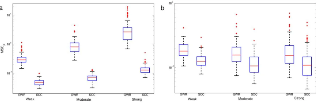
3.6 The T-S relationshipβ1estimated from the (a) SCC method and (b) GWR method . . . 43
3.7 Boxplots ofMSEp for temperature and salinity dataset using SCC, GWR and OLS method . . . 45
4.1 A case study of SST and turbulent heat flux anomalies . . . 53
4.2 The T-Q relationship . . . 54
4.3 Time series of annual mean for (a)αmeso, (b) wind energy, (c) storm track intensity, and (d) variance of mesoscale SST anomalies . . . 57
LIST OF TABLES
TABLE Page
2.1 Estimates ofϕ,σ2andcusing MLE and CL method with different
weight-ing schemes . . . 20
3.1 Spatial range parameters for predictors used in simulation studies. . . 33
3.2 Summary of Study 1 . . . 36
3.3 Summary of Study 2 . . . 38
3.4 The mean and median ofMSEβ andMSEpfor the SCC, GWR and OLS method . . . 45
1. INTRODUCTION
Nowadays the popular usage of geographical information systems (GIS) and global positioning systems (GPS) have led to the increased collection of research data geocoded at accurate locations, in the field of geoscience, econometrics and biological science. This has fueled increasing interest in statistical modeling and analysis with the spatial locations of measurements being taken into account. Spatial statistics is now an important field within statistics.
The main feature of spatial data is the dependence of observations since data observed on proximal locations tend to have similar values, possibly resulting from homogeneous physical dynamics or environmental conditions. Ignoring this spatial dependence may result in incorrect estimation of model parameters and inaccurate predictions.
There are three major objectives for spatial analysis. One of the research goals is to make inferences on the properties of the process. That is, to estimate the parameters de-scribing the spatial dependence structure. Another primary goal is to explain the variability in the process of interest using a set of explanatory variables. One useful framework to achieve this goal is spatial regression. Spatial regression coefficients reveal both the effect of covariates, and provide important information on the relationship between two pro-cesses. The third goal of spatial analysis is that of prediction. That is, predict an outcome at an unobserved location, given the observed values. This dissertation focuses on the first two research goals.
In investigating the properties of a process, conventional likelihood-based model infer-ence methods, such as maximum likelihood estimation (MLE) and Bayesian inferinfer-ence, are computationally expensive for many spatial models with large data sets. As an alternative inference tool, composite likelihood (CL) methods have gained considerable attention in
recent years due to their simplicity and sound asymptotic properties. However, CL estima-tors often result in substantial loss in statistical efficiency with respect to MLE. To improve statistical efficiency or to reduce the computational burden, recent approaches consider the choice of weights in constructing composite likelihood in the context of spatial process. We follow this path, in the first study, to seek an adaptive weight function for composite likelihood with a good balance between computational complexity and estimation effi-ciency.
In dealing with multiple spatial processes, spatial regression models such as Gaus-sian process regression or spatial generalized linear regression models have been widely adopted to address this problem, in which spatial dependence is taken into account by adding a spatial random effect to the (generalized) linear regression model. Regression coefficients in such models are often assumed to be a constant. However, in many prob-lems especially when data are collected across a large region, it is unlikely that a constant regression coefficient can adequately capture the spatially dynamic relationship between response variables and covariates. One example is to have clustered pattern of regression coefficients that abruptly change across the boundary of adjacent clusters but stay rela-tively homogeneous within clusters. Indeed, it is of great interest to many practitioners to identify such clusters that allow them to explain varying associations between the response of interest and covariates. There is no existing method designed to address the clustered coefficient regression. We develop a spatial modeling approach with the ability to capture the spatial structures in the effect of the explanatory variables.
The relationship between response variables and covariates may not only vary in the physical space but also in the spectral space. The latter is quite common in the applica-tions of geophysics as the dynamics controlling the relaapplica-tionship typically changes with the spatial scales. While a knowledge of the scale-dependent relationship is essential to understand the nature of geophysical system, so far no modelling approaches have been
proposed to address these types of problems. In the third study, we extend the varying coef-ficient regression model developed in the second study to the spectral domain, constructing a penalized spectral regression model to estimate the scale-dependent relationship between response variables and covariates.
The rest of this dissertation is organized as follows. In Section 2, we present the study of weighted composite likelihood, focusing on effective estimation of covariance parameters in spatial Gaussian process. Section 3 details the Spatial Clustered Coefficient (SCC) model and its theoretical properties. An extension of the SCC model in the spectral domain is provided in Section 4 with its application to the relationship between sea surface temperature and turbulent heat flux at the air-sea interface. Section 5 summarizes the studies in this dissertation.
2. ON APPROXIMATING OPTIMAL WEIGHTED COMPOSITE LIKELIHOOD METHOD FOR SPATIAL MODELS
2.1 Introduction
There has been much interest in recent years in a form of likelihood type estimation called composite likelihood (CL). It is a weighted product of a collection of component likelihoods such as low dimensional conditional or marginal densities. Because each com-ponent in CL is a valid likelihood object, the corresponding estimating equation obtained from the score function of CL is unbiased under standard regularity conditions. There-fore, the CL inference is known to have well established properties of a likelihood from a misspecified model. Compared to the maximum likelihood (ML) approach, the CL method does not require evaluations of full likelihood functions but only products of low-dimensional marginal or conditional likelihoods, leading to a considerable reduction of computational burden, although a loss of statistical efficiency is generally expected with respect to the ML method.
CL methods have been used in many contexts when it is difficult or computational ex-pensive to evaluate or specify full likelihoods. In particular, various types of CL functions have been introduced in spatial statistics to facilitate computations. For spatial GP models, it is known that the full likelihood function of a GP model involves inversion of ann×n covariance matrix for a data set of sizen, requiring O(n3)operation andO(n2)memory. This can be computationally infeasible for large datasets which are becoming increasingly common in geosciences. [1] compared three CL functions for spatial GP models based on the paired marginal distributions, paired conditional distributions and paired differences. Recently, in [2], the authors proposed to use a composite likelihood function defined as a product of the joint densities of pairwise spatial blocks. For spatial generalized
lin-ear mixed models, the authors in [3] proposed a composite likelihood approach based on marginal densities of pairwise differences of responses; and the authors in [4] proposed a pairwise composite likelihood approach based on bivariate marginal densities. [5] used the composite likelihoods for the inference of a Gaussian max-stable process for spatial ex-treme values, in which the closed-form expressions of the corresponding joint likelihoods are intractable.
As outlined in [6], for a given estimation problem, the choice of a suitable CL function should be driven by statistical and computational considerations. However, it is noticeable that many existing methods of CLs are constructed with equally weighted pairs due to its simplicity. To improve statistical efficiency or to further reduce the computational burden associated with large data sets that have enormous number of pairs, several investigations have considered the choice of weights when constructing CL in the context of a spatial process. One popular strategy is to use binary weights to exclude those pairs whose dis-tances are beyond certain taper range [4, 7]. [8] and [9] consider selecting a taper range by maximizing certain criteria derived from the Godambe information matrix of a CL es-timator. The CL estimators based on binary weights have improved statistical efficiency over equally weighted CL methods. However, these methods ignore dependence among selected pairs and hence can still lead to considerable loss of statistical efficiency. Thus far, very limited work has been done on designing non-binary weights. [8] investigated weighted composite score for a scalar parameter and constructed a weight by minimiz-ing an upper bound of the asymptotic variance of the estimates. They find that the pro-posed weighted CL method performs better than both the binary weighted method and the equally weighted CL method for Gaussian random fields. [10] proposed a joint com-posite estimating function (JCEF) approach through a weight matrix to spatio-temporally clustered data.
likelihood (WCL) method for spatial Gaussian processes. The proposed weight is moti-vated from the optimal weight derived from the theory of estimating equations. It is known that the computational burden in constructing optimal estimating equations is formidable as it requires the inversion of a large covariance matrix of scores. To circumvent the diffi-culty in computing optimal weights, we exploit spatial dependence structures among pairs and develop a sparse matrix approximation method based upon block-diagonal structure and tapering. This leads to a weight function with a good balance between computation complexity and estimation efficiency.
Both the cases with a scalar parameter and multiple covariance parameters are inves-tigated. We develop a weighted profile composite likelihood method that iteratively esti-mates each model parameter using WCL. Our method allows the use of different weights for each individual model parameter to reflect different correlation structures among pairs of score functions.
This section is organized as follows. In Section 2.2, we review some basics for compos-ite likelihoods and spatial Gaussian process relevant to this study, and then introduce our methods for efficient covariance estimation. Section 2.3 illustrates the performance of our method through a number of simulation studies. An application to real data is presented in Section 2.4, using the yearly total precipitation anomalies dataset [11]. Conclusions are summarized in Section 2.5 followed by discussion.
2.2 Methodology
2.2.1 Composite likelihood
Consider a parametric statistical model with probability density function{f(z;θ),z ∈
Z ⊆ Rn}, where θ is a p-dimensional parameter vector to be estimated. Denoting by {A1,A2, ... ,AK} a set of marginal or conditional events, composite likelihood is a
weighted product of the likelihood corresponding to each single event [6] CL(θ;z) = K ∏ k=1 f(z∈ Ak;θ)ωk, (2.1)
wheref(z ∈ Ak;θ)is the likelihood of event Ak and{ωk,k = 1, ... ,K}is a set of non-negative weights to be chosen. The associated weighted composite log-likelihood is
cℓ(θ;z) = K ∑ k=1 ωkℓk(θ;z), (2.2) whereℓk(θ;z) = logf(z∈ Ak;θ).
CL in (2.2) is a universal expression of the weighted composite log-likelihood allowing for combinations of marginal and conditional densities [12]. For example, a special form of CL is compounded based on pairwise differences between observations
cℓ(θ;z) = N ∑ t=1 ∑ i̸=j wijℓij(θ;z (t) i −z (t) j ), (2.3)
wherez(ti )is the sample of thet-th replicate forzi.
Consider a spatial random fieldZ(s)that is modeled as a Gaussian process with mean
µ(s)and a covariance functionC(s,s′;θ). For example, an exponential covariance func-tion takes the formC(s,s′;θ) =σ2exp(|s−s′|/ϕ), whereσ2is the variance parameter,ϕ
is the spatial dependence range parameter. It is well known that the data likelihood withn observed locations involves the inversion of ann×ncovariance matrix. The computational cost can be very intensive or even prohibitive whennis large.
CL offers an alternative inference approach that only requires low-dimensional like-lihood calculation and hence has a clear computational advantage over full likelike-lihood. Indeed, the computational cost for considering all possible pairs is of orderO(n2). In this
paper, we focus on constructing a WCL based on pairwise differences for the inference of covariance parameters while assuming µ(s)is a constant in the rest of the paper. We remark that it is relatively straightforward to extend the proposed method by including a mean model for µ(s)following similar strategies as in restricted maximum likelihood (REML).
LetUij,t = Z(si,t)−Z(sj,t),i ̸= j,t = 1,· · · ,N, the differences between any two observations of the t-th replicate. Then, we have Uij,t ∼ N(0, 2γij(θ)), where γij(θ) = var[Z(si)−Z(sj)], also known as the variogram in spatial statistics. The composite likeli-hood of the pairwise difference in (2.3) can be expressed ascℓ(θ) = ∑Nt=1∑i̸=jwijℓij,t(θ), whereℓij,t(θ) = −{logγij(θ)/2 + [Uij,t]2/(4γij(θ))}.
Composite likelihood can be justified within the framework of the theory of estimating functions. LetbθCL be the maximum composite likelihood estimator ofθ. Clearly,bθCL is also the solution of the following composite score equations,
s(θ;z) =∇cℓ(θ;z) =∑ i̸=j
wijsij(θ;z) = 0, (2.4)
where∇denotes the gradient obtained by differentiation with respect toθ. Heresij(θ;z) = (∑Nt=1∇θ1ℓij,t(θ;z),· · · ,
∑N
t=1∇θpℓij,t(θ;z)), representing score contributions from each
pair(i,j).
Sinces(θ;z) is a linear combination of the scores associated with each of the likeli-hood terms, it is indeed an unbiased estimating equation satisfyingE{s(θ,z)}= 0under standard regularity conditions [6]. Therefore, under the theory of the unbiased estimating function, the maximized composite likelihood estimator θCLˆ is a consistent and unbiased parameter estimator [4, 6],
in distribution as N → +∞, where G(θ) = H(θ)J(θ)−1H(θ) known as Godambe infor-mation [13] or sandwich inforinfor-mation,H(θ) =E{−∇2cℓ(θ)}andJ(θ) = var{∇cℓ(θ)}.
Despite its sound asymptotic properties, the estimation method using CL typically results in loss of statistical efficiency compared with the maximum likelihood estimator counterpart. Indeed, CL can be viewed as a misspecified model, and hence may not attain the Cramér-Rao lower bound [12]. Nevertheless, efficiency gain might be achieved by carefully designing ways to construct composite likelihood while keeping low computa-tional cost [10, 14]. Below, we seek to construct a WCL to provide a good compromise between computation cost and estimation efficiency.
2.2.2 Approximate optimal weighted composite likelihood
In this paper, we present a weighting strategy with the goal to improve the efficiency of CL by exploiting the theory of optimal estimating equations [15]. Stack all the individual score vectorsij(θ)of sizepinto a column vectorS(θ)of sizepn(n−1)/2. Now letW(θ), a pn(n− 1)/2 ×p matrix, be the weighting function of θ. Then Q(θ) = W(θ)TS(θ) defines a class of valid unbiased estimating functions. For example, the equally weighted CL corresponds to the case where W(θ) is a binary matrix1n(n−1)/2⊗Ip. Letθw be the root of the estimating function Q(θ)with weight matrixW, the approximate asymptotic covariance matrix ofθw is given by
E{∇Q(θ)}]−1E{Q(θ)Q(θ)T}]−1E{∇Q(θ)}]−T (2.6)
In the class of estimating functions Q(θ), the approximate covariance matrix in (2.6) is minimized with respect to the partial ordering of nonnegative definite symmetric matrices (see, [15]) when
Although the weight matrix with the above form combines score vectors in an optimal way and leads to efficient estimators, it is rarely used in practice. Indeed, Cov(S(θ)) is apn(n−1)/2×pn(n−1)/2matrix, whose inversion requires O(n6)of computational complexity, making it computationally prohibitive for large spatial data sets. Below, we seek strategies to approximateWOpt to circumvent computational difficulties.
We first consider the case in which parameter θ is a scalar. In this case, we stack sij(θ;z),j ̸= i into a vectorS(θ)of sizen(n−1)/2. Following (2.7), the optimal weight WOpt = −ET{∇S(θ)}Cov(S(θ))−1
. Under mild regularity conditions, −E{∇Sij(θ)} = Var(Sij(θ)), i.e., the diagonal entries of Cov(S(θ)). Rewrite Cov{S(θ)}= DCorr{S(θ)}D, where D is a diagonal matrix proportional to the square roots of the diagonal entries of Cov(S(θ)). The optimal weightWOpt can be expressed as
WOpt = D−1Corr(S(θ))−1D1. (2.8)
Clearly, equally weighted CL essentially corresponds to the case where correlations among score elements are treated as zeros. However, such assumptions are unrealistic for spa-tial models in which pairs of scores constructed on spaspa-tial differences often show non-negligible dependence.
We seek methods to approximate the optimal weight function that takes into account correlations among spatial pairs while keeping the computation at a low cost. To motivate such an approximation, we investigate the pattern of the weight functionWOpt(θ)and the covariance of score functions below. First note that−ET{∇S(θ)}is a vector of sizen(n− 1)/2 with each element to beIij, the marginal Fisher information of the likelihood for a spatial pair(i,j). The marginal information contribution from each spatial pair is expected to vary as the distance between i and j. In fact, for a spatial Gaussian process model with variogramγij, Iij = N
[γij(1)(θ)]2
2γ2
ij(θ)
information gain by adding a pair (i,j) from a weighted CL is bounded by the marginal informationIij. Therefore, this motivates us to taper pairs if their marginal information is below certain threshold before constructing WCL. For example, whenγij is an exponential variogram function and the goal is to estimate the range parameter while fixing σ2, it is easy to show that the marginal information is a monotone decaying function of distance, which indicates that pairs with distances beyond certain taper range, denoted asτ, can be excluded since their contributed information is minimal.
LetS(θ)taper denote the score vector stacked from the taperedsij(θ). We next examine the pattern of the correlation matrix of the score function Cscore,taper = Corr{S(θ)taper}. Apparently, the dimension of this correlation matrix is greatly reduced thanks to taper-ing. To further reduce computation, a natural idea is to seek strategies to approximate Corr{S(θ)} by only keeping elements with large correlations. Note that for the spatial problem we consider here,
Corr{Sij(θ),Sℓk(θ)}= {γiℓ(θ)−γjℓ(θ) +γjk(θ)−γik(θ)} 2
4γij(θ)γℓk(θ)
. (2.9)
It can be proved that for a given pair(i,j),
Corr{Sij(θ),Sℓk(θ)} ≤max{Corr(Sij(θ),Sℓ1ℓ2(θ))} (2.10)
holds for any ℓ1 ∈ {i ̸= j} and ℓ2 ∈ {/ ℓ ̸= k}. This inequality suggests that two pairs achieve the largest correlation when two vertices from each pair coincides with each other. Motivated by this finding, for a score function corresponding to a given pair (i,j), we propose to keep its correlation with{(i,ℓ)}, for all{ℓ : diℓ < τ}and set correlations for pairs without shared vertex to be 0. It clearly has an advantage over equal-weight CL which
completely ignores correlations among pairs. By using a more accurate approximation of the optimal weights,WBT(ϕ)is expected to achieve greater statistical efficiency compared with other WCL methods.
We acknowledge that this approximation ignores correlations among pairs without shared vertices. We explain below why it is necessary to do so for the sake of computation efficiency. Under a proper ordering of pairs, the approximation method described above results in a block diagonal matrix approximation to the correlation matrixCscore,taper, de-noted asCscore,BT. LetMdenote the number of blocks, which equals the number of unique vertices from all remaining pairs after tapering. For a given order of these vertices from 1toM, them-th block is the correlation matrix of a set of two pairs{(m,j), (m,ℓ)}, for
{j ̸= ℓ > m,dmj < τ,dmℓ < τ}. Compared to the original full correlation matrix of the score vector for all pairs, the computational cost associated with this approximated correlation matrix is greatly reduced for two reasons: first the dimension of the matrix is substantially reduced from the total number of pairs to the number of close pairs only; and the approximated correlation of the close pairs has block diagonal structures, whose computation can be handled efficiently and in parallel.
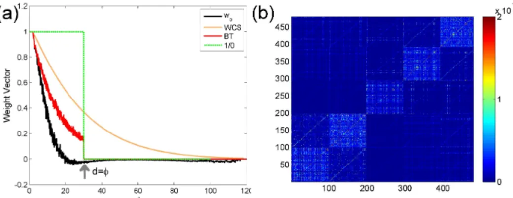
To illustrate the above idea, below we plot the pattern of the covariance matrix of the score function Cscore,taper through a simulation. We generate 100 independent replicates of realizations from a spatial Gaussian process at 100 randomly selected locations from [0, 100]×[0, 100]. An exponential covariance function is used with the range parameter
ϕ = 30and the varianceσ2= 1(no nugget effect). We first consider estimatingϕassuming
σ2is known. Figure 2.1(a) shows the averaged score correlation matrixCscore,taper for the re-ordered remaining pairs after tapering. A notable feature forCscore,taper is that the value in its block diagonals are generally significantly larger than the non-block diagonals, which justifies our approximation strategy by only considering block diagonal correlations that capture dependence for two pairs that share a vertex.
Figure 2.1: Weights for composite likelihood. (a) Various weights as a function of distance of pairs. (b) The covariance matrix of scores Cov(S(θ))based on exponential covariance withσ2 = 1andϕ= 30.
With the use of the approximated score correlation matrixCscore,BT, we propose a new weighting function termed as block-tapering (BT) weight
WBT(θ) =−ET{∇S(θ)taper}Cscore,BT(θ)−1, (2.11)
for all pairs withdij < τ, and 0 otherwise.
Using the same simulated dataset as above, we evaluate the proposed weight func-tionWBT (referred to as the BT-WCL method) and compare it with various other weight functions, including a binary 1/0 weight by tapering distant pairs (denoted as W1/0(ϕ), referred to as 1/0-WCL), an adaptive weight WWCS(θ) = diag{−E[ℓ(2)ij (θ)]} (referred to as the WCS method) proposed by [8], and the optimal weightWOpt(ϕ)as a benchmark. ClearlyWOpt(ϕ)appears to have a strong decreasing trend as distancedas shown in Figure 2.1(b), which is consistent with the findings in previous studies that distant pairs are nearly uncorrelated and hence contribute little information in terms of estimating range parame-ter. For the examples considered here with the exponential covariance, indeed the optimal weightWOpt(ϕ)decreases from 1 (d = 0) to 0.05 atd ≥ ϕ, suggesting the use ofϕ as a
threshold to guarantee little loss of efficiency. It is also noticeable that the weightWBT(ϕ) is in greater agreement with the curveWOpt(ϕ)thanWWCS(ϕ)orW1/0(ϕ). This finding is not surprising considering thatW1/0(ϕ)is essentially equivalent to the weight by approxi-mating Corr(S(ϕ))taper as an identity matrix, andWWCS(ϕ)is essentially equivalent to the weight by approximating Cov(S(ϕ)) as an identify matrix. Ford ≥ ϕ, WOpt(ϕ),WBT(ϕ) and W1/0(ϕ) are nearly zero while WWCS(ϕ) is still significantly greater than zero. For d ≤ ϕ, WOpt(ϕ),WBT(ϕ) and WWCS(ϕ) all decrease fairly smoothly with spatial lag d. But the decay rate ofWBT(ϕ)is much closer to that of theWOpt(ϕ)than that ofWWCS(ϕ). These findings imply that the our proposed method uses a more accurate approximation to the optimal weight and hence is expected to improve statistical efficiency compared to the 1/0 weight and WCS weight methods. We will further demonstrate the utility our method in Section 2.3 through numerical simulations.
We now consider the case with multiple parameters. The optimal weight in this case involves the inversion of Cov(S(θ)), apn(n−1)/2×2n(n−1)/2matrix. In view of the computational expense of the joint optimal weight in (2.8), we propose to iteratively esti-mate model parameters following a similar spirit as in the profile likelihood method. That is, given current values of (bσ2, ˆϕ), we calculate a weighting function for each individual parameter and then estimate the parameter by maximizing the weighted profile composite likelihood. For example, assume both the range parameterϕand the varianceσ2 are now unknown, we estimate model parameters according to the following procedures:
(1) Start from some initial values of(σb2, ˆϕ). One way is to obtain preliminary estimates of(σb2, ˆϕ)using fast estimation methods such as the tapered equally-weighted CL. (2) Givenbσ2, updateϕˆusing the BT-WCL method, and
The entire procedure repeats steps (2) and (3) until convergence. Of course, there is no guarantee that convergence to a fixed pint of the iterative process will occur, especially when parameters are not orthogonal [16]. However, our simulation studies show that in general convergence to a fixed point is rapid.
2.3 Simulation studies
We design a number of simulation studies to investigate the use of the BT-WCL method for the inference of spatial Gaussian process regression models.
2.3.1 Simulation 1: only range parameter is unknown
We simulateN process realizations from a Gaussian process with exponential covari-ance function at n spatial locations. We set the true value of the variance parameter σ2
to be 1 and experiment with a range of true values of the range parameter ϕ. We first consider the situation where only the range parameter is unknown while the other param-eters are fixed. We compare the estimators under different CL methods via Monte Carlo simulation results by setting N = 1000 replicates. We set n = 100 spatial locations to make it computationally feasible to obtain the results of the optimal weight CL esti-mator WOpt(ϕ) for our comparison analysis. To avoid numerical singularities, locations of observations are generated following a sampling approach similar to the one in [11]. Specifically, a two-dimensional regular grid is first generated with increments of 2 over the domain [0,√100N] ×[0,√100N]. Then each grid point is perturbed by adding a random noise, uniformly distributed on[−0.5, 0.5]to each coordinate. In this case, each perturbed gridpoint is at least 1 unit away from any of its neighbors. Finally, nlocations are randomly chosen from the perturbed grid points without replacement.
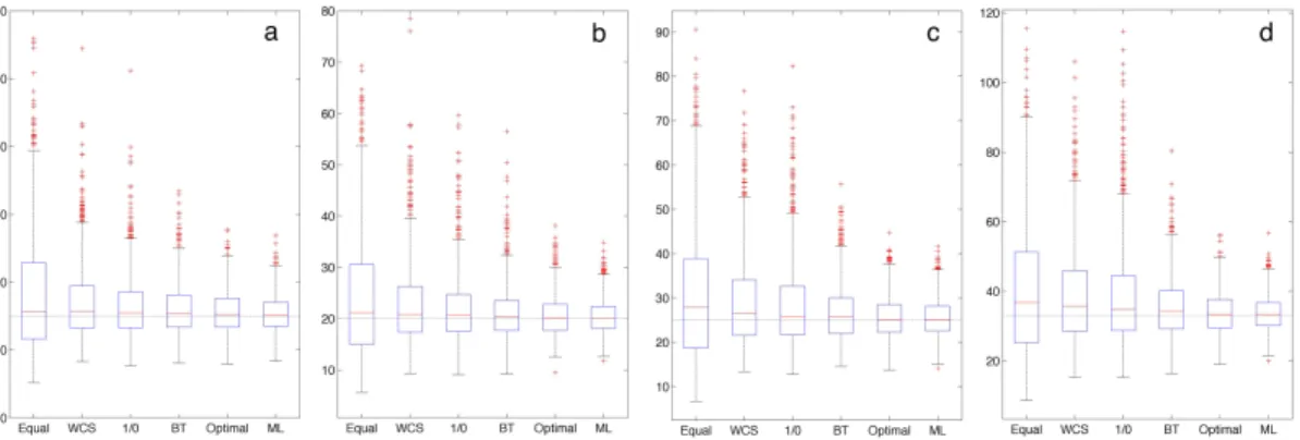
Figure 2.2 presents the boxplots of the estimates using the five CL methods (Eq-WCL, WCS,1/0-WCL, BT-WCL, Opt-WCL) and the MLE method for various values ofϕ. No strong biases are observed across all the CL estimators. In contrast, evident differences
Figure 2.2: The boxplots of estimates for ϕˆ using various methods. Those include Eq-WCL, WCS, 1/0-Eq-WCL, BT-Eq-WCL, Opt-WCL and MLE when (a) ϕ = 15, (b) ϕ = 20, (c)
ϕ = 25 and (d)ϕ = 30with observation numberN = 100. Dot-dashed horizontal lines represent the true value ofϕ. The variance is known asσ2 = 1.
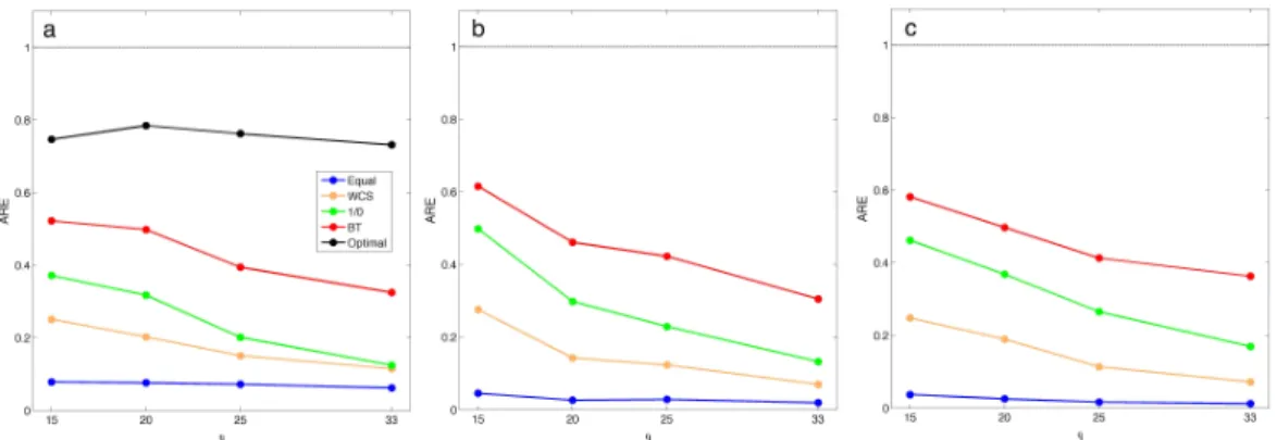
in standard error for the6estimators are observed from the boxplots. Generally, the stan-dard error for all estimators becomes larger as the range parameter ϕ increases. We also calculate the relative efficiency (RE) between each of the 5 versions of composite like-lihood (WBT(ϕ),Wequal(ϕ), W1/0(ϕ) and WWCS(ϕ), WOpt(ϕ) ) and the MLE, denoted as MSE(·)/MSE(MLE), and report the results in Figure 2.3 (a). As expected, the highest RE among the five CL methods is achieved by using the Opt-WCL method. Moreover, all of the three adaptive weight CL approaches (BT-WCL, WCS, 1/0-WCL ) show better performance than the equally weighted CL. Among them, the estimates obtained from the proposed BT-WCL estimator yield a value of RE closest to that of the Opt-WCL estimates, which is consistent with the findings in Section 2.2.2. In this study, the RE of the 1/0-WCL and the WCS are generally30%−65%lower than that of the BT-WCL. We also examine the performance of these CL methods for two larger numbers of locationsn = 400 and n = 1000, respectively. The results of theWOpt(ϕ)are not shown since the computation becomes formidable for largen. Overall, the results in Figure 2.3(a) and (b) indicate that
the use of the BT weight achieves significant efficiency gains over the other CL methods in parameter estimations. Efficiency gain also seems to be stronger as spatial dependence range becomes shorter.
Figure 2.3: The relative efficiency (RE) of CL estimates for ϕ using different weighting schemes. RE are calculated in case of (a)N = 100, (B)N = 400and (c)N = 1000. The variance is known asσ2 = 1. Dot-dashed horizontal lines representRE = 1.
2.3.2 Simulation 2: all parameters unknown
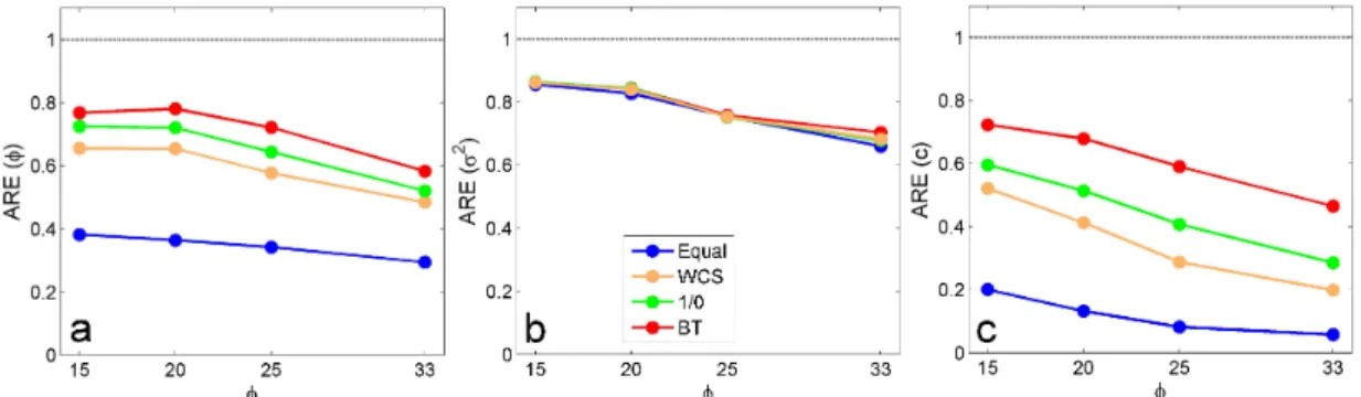
To examine the performance of the iterative CL method for the case with multiple parameters described in 2.2.2, in this study we consider a similar simulation design as the one in 2.3.1 but assume both ϕ and σ2 are unknown. For each of the 1000 simulation replicates, we generate data at N = 1000sampling locations. We compare the results of the estimates of ϕ and σ2 using the (iterative) BT-WCL, Eq-WCL, 1/0-WCL, and WCS methods. In addition, we also include the results of the estimates of c = σ2/ϕ, whose MLE has been shown to be a consistent estimator under the fixed domain asymptotics [17]. Figure 2.4 shows the RE for each estimator. Overall, we observe similar results as in the case where σ2 is known. The (iterative) BT-WCL approach outperforms the Eq-WCL,
1/0-WCL, and WCS method. For ϕ andc, all the adaptive weighted CL methods have substantial improvement in RE over the equally weighted CL method, especially for spatial GP with smaller scale spatial dependence structures. But for σ2, the relative efficiencies (RE) of the estimates from various CL methods are comparable with each other.
Figure 2.4: The relative efficiency (RE) of CL estimates for different parameters. Esti-mates for (a)ϕ, (b)σ2and (c)c are calculated using different weighting schemes in case of N = 1000. Dot-dashed horizontal lines representRE = 1.
2.3.3 Simulation 3: computational efficiency
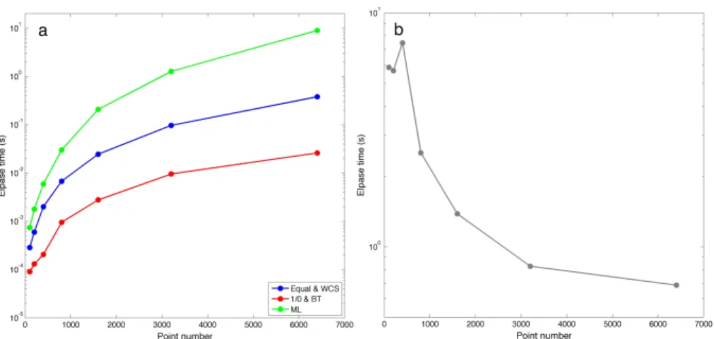
We have shown that the BT-WCL method achieves significant statistical efficiency gain in the above simulations. We now focus on examining the performance of the BT-WCL in terms of its computational efficiency. We use the simulation designed as study 1 but varying the number of locations K from 100 to 6400 to compare the computation time associated with each different methods. All computations are carried out on a 2.3GHz four-core processor with 16GB of memory.
Figure 2.5(a) shows the computation times required for a single evaluation of the full likelihood function and the composite likelihood function associated with each of the WCL methods. These are calculated by averaging over 100 repetitions of evaluation. Note that
Figure 2.5: Computational burden for different weights. (a) The computation time for a single evaluation of full likelihood function and CL function with different weighting schemes. (b) The ratio of computation time for computing BT weight to that for evaluating composite likelihood.
the calculation of composite likelihood is of the same order for the BT-WCL and the 1/0-WCL method if the same taper range is used. This is also the case for the WCS and the Eq-WCL approach in which all pairs of observations are included. All the CL estimators result in a reduction of computational time compared to the MLE as expected. The computational gains of the BT-WCL are substantial: with 6400 observations, the computation time for the BT-WCL is only0.3%of that for the MLE. It also outperforms BT-WCL the equal-weighted CL method and WCS method thanks to the exclusion of distant pairs: the computational time for the BT-WCL is only 7% of that for the WCS and equal-weighted CL method. It is also noticeable that the computational gain becomes more pronounced when increasing the number of observations, making it desirable for large spatial data sets.
We remark that the computation of the BT-WCL estimator requires precomputing the BT weight matrix to be used for the evaluation of the composite likelihood function. Therefore, we also examine the extra computational cost associated with the
computa-tion of the BT weight matrix. Figure 2.5(b) shows the ratio of the computacomputa-tion times between calculating weights and composite likelihood functions given weights. The result indicates that the computation cost is mainly attributed to CL function evaluation asn be-comes large. The computation of the inversion of the sparse block matrix Cov(S(θ))used in BT-WCL does not cause a substantial increase in computational burden.
2.4 Application to precipitation data
We illustrate the BT-WCT method using the yearly total precipitation anomalies at 7,352 weather stations from the year 1962 in United States. This large, irregularly spaced spatial data was used by [11]. The yearly totals precipitation anomalies is yearly totals standardized by the long-term mean and standard deviation for each station. [11] men-tioned it shows no obvious nonstationarity and anisotropy. Therefore, we fit to the data Gaussian process model with an exponential covariance function (without nugget effect), which is stationary and isotropic.
Table 2.1: Estimates of ϕ, σ2 andc using MLE and CL method with different weighting schemes. The bottom row presents the computation time required for a single evaluation of full likelihood function and composite likelihood.
Parameter MLE BT-WCL Eq-WCL WCS 1/0-WCL
ϕ(km) 65.9 101.4 203.8 162.8 145.8
σ2 0.72 0.77 0.78 0.77 0.77
c 0.011 0.008 0.004 0.005 0.005
Times(s) 12.64 0.03 0.47 0.47 0.03
The estimates for ϕ, σ2, and c using MLE and CL method with different type of weights are provided in Table 2.1. The MLE for ϕ and σ2 are 65.9 and 0.722, respec-tively, while the CL estimators are 101.4 and 0.765, larger than MLE. Among various
weighted CL estimates, BT-WCL estimate is the closet to MLE. It is not surprising that the equally weighted CL estimate is furthest from the MLE. As to the computation cost, the CL estimators lead to a substantial reduction of computational time compared to the MLE (Table 2.1). The MLE requires 12.64 seconds to evaluate a single likelihood, which is about 400 times of the cost of BT-WCL.
2.5 Conclusions and discussion
The section addressed the problem of estimating covariance parameters of spatial Gaussian processes when the dataset is large and irregularly spaced. We have proposed a new adaptively weighted CL method, i.e., the BT-WCL method. The BT weight is an ap-proximation to the optimal weight derived from the theory of optimal estimation equation. It is calculated with the strategy of combining block-diagonal feature and tapering. This weighting scheme leads to a considerable reduction of computational burden and retains sound estimation efficiency.
We have shown the utility of our method through simulations and data examples. In this section, we only investigate the use of a BT weight for the estimation of a spatial Gaussian process with exponential covariance function. It is possible to extend the tech-niques to more generalized covariance function with decay correlation with distance. In-deed, we also find that the block-diagonal feature of the covariance of scores exists for the model with power exponential covariance in an unreported simulation study. A challenge in some of these cases will be to analytically evaluate the covariance of scores. However, sampling or subsampling based methods might be adopted to estimate them as done in [18] and [10]. Finally, our method of estimating the optimal weight in WCL by blocking and tapering also has great potential to be applied for non-Gaussian spatial data in the context of copula models or spatial generalized linear models. These topics will be investigated in future work.
3. SPATIAL CLUSTERED COEFFICIENT REGRESSION MODEL
3.1 Introduction
Numerous problems in environmental, earth, and biological sciences nowadays involve large amounts of spatial data, obtained from remote ground sensors, satellite images, scien-tific climate computer models, geographic information systems, public health and spatial genetics, etc. In many such applications, a main problem of interest is to explain the vari-ability in a response variable observed over the region of interest using a set of explanatory variables, considering spatial dependence of observations.
Spatial regression models such as Gaussian process regression or spatial generalized linear regression models have been widely adopted to address this problem, in which spa-tial dependence is accounted for by adding a spaspa-tial random effect to the (generalized) linear regression models. Regression coefficients in such models are often assumed to be a constant. However, in many problems especially when data are collected across a large region, it is unlikely that a constant regression coefficient can adequately capture the spa-tially dynamic relationship between response variables and covariates. One example is to have clustered pattern of regression coefficients that abruptly change across the boundary of adjacent clusters but stay relatively homogeneous within clusters. Indeed, it is of great interest to many practitioners to identify such clusters that allow them to explain varying associations between responses of interest and covariates.
Our specific motivation problem is from an important scientific question in oceanog-raphy. Geophysical fluids (i.e., air and sea water) consist of distinct fluids masses [19]. Within each fluids mass, the physical and chemical properties are relatively homoge-neous. But they change rapidly across the narrow boundary between adjacent fluids masses (termed as fronts in geoscience). Such a phenomenon is formed as a result of nonlinear
nature of geophysical fluids dynamics and ubiquitous in the atmosphere and ocean [20]. When exploring the relationship between features of fluids, it is likely that the relationship will change abruptly across the fronts. One notable instance is the relationship between temperature and salinity of sea water (referred to as the T-S relationship henceforth). In oceanography, temperature and salinity are two important features of water masses and strongly affect the ocean currents [19]. Knowledge of spatial distribution of T-S relation-ship in the ocean provides important information on the movement and extent of individual water masses. Such information can be further used to monitor the pathway and strength of meridional overturning circulation (MOC) which plays a key role in the global climate system. It is desirable to built a model with the ability to capture such spatial structures in the effect of the explanatory variables.
However, to the best of our knowledge, there are very limited work on spatially clus-tered coefficient regression models. Thus far, literature on spatially varying coefficient models mainly focus on smoothly varying coefficient models. Geographically Weighted Regression (GWR) [21] and Spatially-Varying Coefficients (SVC) model [22] are two popular models of this type. GWR is an ensemble of spatial local regression models fitted separately. That is, a linear regression model is fitted at each spatial point, giving greater weights to the closer points. In SVC model, the spatially-varying coefficient surface is modeled as a multivariate spatial process with stationary specification. The SVC adopts a Bayesian approach with posterior inference for all attainable model parameters and thus offers a richer inferential framework. [23] and [24] compare these two methods and sug-gest that SVC generally produces more accurate inferences on the regression coefficients especially in the presence of strong colinearity among explanatory variables. However, the superiority of SVC in estimation accuracy is at the cost of much higher computational burden due to the requirement of Metropolis MCMC. For a moderate data size of 1000 points and three spatially varying coefficients, it may take several days to collect sufficient
MCMC samples [23]. This largely limits its application to large spatial datasets which become more and more common with advances in observational techniques. Moreover, both GWR and SVC implicitly or explicitly assume stationarity in the spatially-varying coefficient surface over the space as neither the weighting function in GWR or covariance function of the coefficient process in SVC depends on the location. However, such a sim-ple assumption would not be consistent with the complicated spatial structure of regression coefficients in certain applications. The coefficients could vary more rapidly in some parts of the domain than others.
In this section, our main contribution is to propose a new spatial modeling approach to estimate regression coefficients with the presence of a spatial pattern, especially a clustered pattern, influencing the effect of the explanatory variables without assuming stationarity in effect. The proposed method, called Spatially Clustered Coefficient (SCC) regression, employs penalized least square by penalizing the pairwise difference of regression coeffi-cients between two locations that are connected by an edge in the graph. Edge selection in our problem is challenging since there is no clear ordering of spatial points. Previous stud-ies such as 2d (gridded) fused lasso [25] considers all the edges in a lattice graph, which can have costly computational complexity for large spatial data sets. We implemented a spatial graph based on minimum spanning trees (MST). Two coefficients with locations connected by a MST tends to be similar. Therefore, the SCC model can capture the spatial structures in coefficients by encouraging the homogeneity of the coefficient on proximate locations. Even for the smoothly varying coefficients, we will see in the simulations that SCC model has strong local adaptivity and can also accurately detect a spatially highly variable pattern. With this property, the SCC model allows researchers to explore the spa-tial structures in regression coefficients either clustered or smoothly varying. In practice, the proposed method is computationally highly efficient, thanks to the use of MST and transformation that reduces the problem to a usual lasso-type optimization with n − 1
penalty terms for a spatial data set of sizen.
The rest of the section is organized as follows. Section 3.2 details the Spatial Clus-tered Coefficient (SCC) model and discusses theoretical properties of SCC. In Section 3.3, a series of simulation studies are designed to illustrate the performance of SCC. An appli-cation of the method is presented in Section 3.4 using the aforementioned temperature and salinity data in the Atlantic basin. Section 3.5 summarizes the major conclusions of this study followed by discussion. Related proof are provided in the Appendix A.
3.2 Methodology
3.2.1 Spatially clustered coefficient model
Suppose we observe spatial data{(x(si),Y(si)),i = 1, ... ,n}at locations s1, ... ,sn ∈ R2, where the response variableY(si) is assumed to be spatially correlated and x(si) = (x1(si), ... ,xp(si))Tis the p-dimensional vector of explanatory variables for the observation located at si. The intercept can be included by defining xp(si) = 1 for i = 1, ... ,n. Consider the standard linear regression,Y(si) = x(si)Tβ+ϵ(si), whereβ = (β1, ... ,βp)T is the vector of regression coefficients andϵ(si)’s are independently identically distributed random noises with mean 0and variance σ2. Without loss of generality, we assume that the explanatory variables are standardized to have mean0and unit variance.
The extension of the linear regression model to allow spatially varying regression co-efficients is straightforward,
Y(si) =x(si)Tβ(si) +ϵ(si). (3.1)
However, in many spatial datasets, it is very common to observe only one or a limited number of replicates at each location, making the above model ill-posed if without any assumptions on β(si). Indeed, strong spatial patterns ofβ(si) do exist since association
between response variables and explanatory variables at nearby locations are expected to be highly homogeneous. This motivates us to assign a regularization function for β(s) utilizing their spatial homogeneity patterns.
Specifically, we propose to estimateβby minimizing the following objective function n ∑ i=1 {Y(si)− p ∑ k=1 xk(si)βk(si)}2+ p ∑ k=1 ∑ (i,j)∈E Pλ(|βk(si)−βk(sj)|), (3.2)
whereEis a set of coordinate pairs.
The termPλ is a penalty function to encourage homogeneity between two regression coefficients if their corresponding locationssi andsj are connected by an edge inE. Here
λis a regularization parameter determining the strength of penalization. The selection of the penalty functionsPλ, the edge setEand tuning parametersλare three key ingredients in the model in (3.2). Below, we discuss strategies to address these problems.
3.2.1.1 Selection of the penalty functionPλ
There are various forms of penalty functions encouraging sparsity in the literature of variable selection. The simplest and perhaps the most widely adopted one is the Lasso [26] that employs anL1-penalty of the form
Pλ(t) =λ|t|. (3.3)
As the penalty (3.3) is a convex function, efficient convex optimization algorithms can be readily applied. In this case, theL1 penalty enforces sparsity of the difference in two edge-connected coefficients. This method allows the estimation of regression coefficients with a spatially piece-wise constant if edge sets are selected appropriately to incorporate spatial information. The non-zero elements of the estimated|βk(si)−βk(sj)|correspond to boundary points, whereas any two edge-connected coefficient with zero difference
be-long to the same cluster. Naturally, spatial cluster for each explanatory variable can be automatically detected. However, as Lasso assigns large penalties to large values oft, it tends to underestimatet, in our case, the difference in two regression coefficients, when its true value is large. To remedy this flaw, various penalty functions have been proposed, in-cluding adaptive Lasso [27], smoothly clipped absolute deviation (SCAD) [28], minimax concave penalty (MCP) [29], and reciprocal L1-regularization (rLasso) [30]. Adaptive Lasso assigns larger weights to the terms with small values in the L1penalty. SCAD and MCP adopt some concave functions that converge to constants as the penalized term be-comes large. The rLasso uses a class of penalty functions that are decreasing in (0,∞) with a discontinuity at 0 and converging to infinity when the penalized term approaches zero. These two forms have smaller estimation errors compared to Lasso, which, however, is at the expense of considerable increase in computational cost. Therefore, in practice, penalty functions are often selected by weighing a trade-off between statistical efficiency and computational complexity for specific problems. It should be noted that the reduction of computational burden is critically important in spatial analysis as large datasets have become common in diverse fields such as geoscience, ecology, and econometrics. In this section, we mainly focus on the Lasso penalty to demonstrate the power of SCC method for computational simplicity and conservative comparison. We remark that using more advanced penalty forms may further improve the performance of SCC method.
3.2.1.2 Edge selections based on minimum spanning tree
Here we pay special attention to the selection of an edge setE. In spatial problems, each location is a node in a graph. If we believe that the physical properties of geographical locations with close distance tend to be homogeneous, it is not unreasonable to anticipate similar coefficients for proximate locations. Therefore,Eshould only include the coordi-nate pairs that are close to each other. A simple choice ofEsatisfying this criterion is the
set consisting of neighboring coordinate pairs, i.e., E = {(si,sj) : i = 1, ... ,n;sj ∈ Nsi}
whereNsi is the set representing the neighbors ofsi.
However, it is known that, unlike temporal data, spatial data do not have a natural ordering, making it challenging to constructE.
The neighboring setNsi can be defined using either the nearest neighbor ofsi or four neighbors with common borders for grid data such as in 2D fused lasso. Although such selections of E appear to be natural, they suffer from two evident deficiencies. First, E defined above does not necessarily connect all the data points together. In this case, (3.2) does not reduce to a constant regression coefficients model, when λ → ∞. Second, the set E may include redundant coordinate pairs, imposing great computational challenges [31, 32]. For example, consider a regular grid consisting of n points. The number of penalty terms is2n−2√n, many of which are redundant.
The aforementioned analysis suggests that an appropriate choice for E should only include coordinate pairs close to each other, lead to connectivity of all data points, and have no redundant pairs. One choice ofEsatisfying all the three criteria is the minimum spanning tree (MST). For spatial data, we can construct an undirected graph, a set of vertices connected pairwise by edges, G = (V,E)consisting of the set Vof vertices and the setEof edges. In particular, the vertices correspond to the spatial locations and weights of edges correspond to the distance between two locations. In graph theory, a minimum spanning tree (MST) is a sub-graph that connects all the vertices together without any cycles and with the minimum total edge weight. The edge setEconstructed from the MST automatically satisfies the three criteria by definition and is thus an appropriate choice. We chooseEas the edge set of the minimum spanning tree in this study and the corresponding
penalized least square (3.2) with the Lasso penalty becomes n ∑ i=1 {Y(si)− p ∑ k=1 xk(si)βk(si)}2+λ p ∑ k=1 ∥Tβk∥1, (3.4)
whereβk = (βk(s1), ... ,βk(sn))TandTis a(n−1)×nmatrix constructed from the edge set E in the MST.T has full rank and each row vector of Tonly contains two non-zero elements,1and−1, by this construction.
3.2.1.3 Selection of tuning parameterλ
Whenλ → ∞, the model (3.2) yields a constant regression coefficient; when λ = 0, it reduces to the ordinary least square with all different coefficients across the region. With an appropriateλ, the penalized least square model (3.2) produces clustered regres-sion coefficients. In practice, the optimal λ can be determined via some data-dependent model selection criteria, such as generalized cross-validation (GCV) [33], Bayesian infor-mation criterion (BIC) [34] and extended Bayesian inforinfor-mation criterion (EBIC) [35, 36]. In this section, we use BIC instead of EBIC to chooseλsince the latter tends to produce over-sparsity in the penalized term (the difference of regression coefficients in our model) according to previous studies [30].
3.2.2 Computation
The SCC model (3.2) is an optimization problem. It is easy to implement as it can be transformed into a Lasso, or Lasso type problem after suitable reparameterization. We first consider the transformed parametersθk = (θk(s1), ... ,θk(sn))T,k = 1, ... ,pdefined as
θk = T 1 n1 T βk =Tβe k. (3.5)
Tare orthogonal to the unit vector1. Thus, there is a one-to one transformation between βk andθk. Define a new design matrix as
e
X= [diag(x1), ... ,diag(xp)]Te−1, (3.6)
wherediag(xk)is a diagonal matrix with the diagonal entries xk = (xk(s1), ... ,xk(sn))T. Then the SCC model (3.4) can be rewritten as
∥Y−Xeθ∥22+λ∑
t∈B
|θt|, (3.7)
whereθ = (θT1, ... ,θTp)T andB represents the setB = {t : mod(t,n) ̸= 0}. Henceforth, we will denote∑
t∈B
|θt|as∥θB∥1for neatness.
Therefore, the solution to the SCC model (3.2) with Lasso penalty can be obtained by solving the Lasso problem (3.7) with respect to the parameters θ. Estimators for β are given byβck = eT−1cθk. Many efficient algorithms for the Lasso, such as LARS algorithms [37] and coordinate decent algorithm [38] can be readily applied for the SCC model. In this study, we implement the SCC method using the packageglmnet(both in R and Matlab) which is based on the coordinate descent algorithm.
3.2.3 Theoretical properties
In this subsection, we establish the oracle inequalities for the SCC estimators. As there is a one-to one transformation betweenβk andθk , we present theorem in terms ofθ. Assumptions 1. (a) There is a positive constantC1so thatn−1
n
∑
i=1
e
Xi,t2 ≤C1for anyn>0 andt ∈ {1, ...,n·p}. (b) There is a positive constantΦso that for any vectoru ∈ Rn·p satisfying n∑·p t=1 |ut| ≤ 4√|A|√∑ t∈A u2
cardinality, we have 1 nu T(XeTX)ue ≥ Φ∑ t∈A ut2. (3.8)
Assumption 1 is widely adopted in previous literature [39–42]. Assumption 1(a) re-quires the random variablesVt =n−1
n
∑
i=1
e
Xi,tεito be sub-Gaussian for anyt ∈ {1, ...,n·p}. A sufficient condition for assumption 1(b) to be satisfied is that the restriction of Gram ma-trixXeTXeto columnAis positive definite.
Theorem 1. Suppose that Assumption 1 holds. If λ√n/log(n) ≥ 4√(1 +C2)2C2 1σ2 where C2 is a positive constant for anyn > 0, we have the following inequalities with probability tending to unity asn→ ∞
1 n||Xeθ−Xeθb|| 2 2 ≤ 4λ2n|A| Φ , (3.9) ∥θ−θb∥1≤ 8λn|A| Φ . (3.10)
The detailed proof for (3.9) and (3.10) is provide in Appendix A. We note that for the case of infilling domain, |A| ∼ O(√n)asn → ∞. Accordingly, the right hand sides of (3.9) and (3.10) decrease asymptotically to zero asn→ ∞.
3.3 Simulation studies
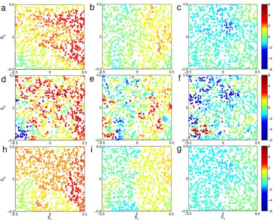
In this section, we present two simulation studies to illustrate the performance of the SCC method under two different scenarios: the true regression coefficients having clus-tered pattern and smoothly varying pattern respectively.
square domain [−0.5, 0.5]×[−0.5, 0.5]. The responses at each location are generated using the linear regression model with two predictors and an intercept:
Y(si) = β1(si)x1(si) +β2(si)x2(si) +β3(si) +ϵ(si), (3.11)
whereϵ(si)iid∼N(0,σ2). We setσ to be 0.1 in the following simulations.
x1(s) andx2(s)are then generated by linearly transforming two independent realiza-tions of a spatial Gaussian process with mean zero and covariance matrix defined from an anisotropic exponential function:
Cov{xk(si),xk(sj)}= exp
( − √ (sh,i−sh,j)2 ϕ2h,k + (sv,i −sv,j)2 ϕ2v,k ) ,k = 1, 2, (3.12)
where (sh,i,sv,i) is the coordinate in the horizontal and vertical direction and (ϕh,k,ϕv,k) is the anisotropic range parameter. Specifically, suppose x1,0(s) and x2,0(s) are the two independent realizations. We letx1,0(s) =x1(s)andx2,0(s) =r x1,0(si) +√1−r2x2,0(si), allowing for the colinearity between the two spatially varying predictors. In the following analysis, we letr = 0.75, corresponding to moderate colinearity.
We remark that numerical data analyses in previous works often generate the value of predictors from a white noise process, corresponding to the special case (ϕh,k,ϕv,k) = (0, 0)[23, 24]. However, such a design of independent variables is far from the reality for spatial data. For example, most of the variables used in geoscience, such as temperature, precipitation, wind speed, ocean primary productivity, and dissolved oxygen in the sea water, have evident spatial structures [19]. When serving as predictors of a regression model in numerical studies, they should be generated from spatially-correlated processes. In the following simulation studies, we reveal that the spatial correlation of predictors will have a profound influence on the efficiency of estimation and prediction.
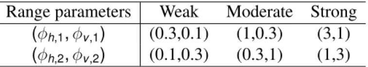
We use Gaussian processes to produce predictors, considering various extent of spatial correlation. Three combinations of range parameters(ϕh,k,ϕv,k), corresponding to weak, moderate and strong spatial correlation, are provided in the Table 3.1. To avoid loss of generosity, we allow distinct spatial structures for different predictors by assigning differ-ent values of (ϕh,k,ϕv,k) for differentk. For each value of (ϕh,k,ϕv,k), we simulate 100 datasets. In each dataset, we randomly select 1000 data points out of the 2000 data points for estimation with the remaining data points held-out for prediction.
Table 3.1: Spatial range parameters for predictors used in simulation studies. Range parameters Weak Moderate Strong
(ϕh,1,ϕv,1) (0.3,0.1) (1,0.3) (3,1) (ϕh,2,ϕv,2) (0.1,0.3) (0.3,1) (1,3)
In both studies, we compare the results with those of GWR. For the GWR method, the regression coefficients at locationsiare estimated byβ(si) = (XTW(si)X)−1XTW(si)Y where X is a n × p matrix with x(si) as the i-th row and W(si) is a diagonal matrix determined from a chosen spatial kernel function. Here we employ an exponential spatial kernel function with the optimal range parameter estimated through cross-validation. We use the packages glmnet to implement SCC method and the package gwr to implement GWR (both packages are available in R and Matlab). The results of the SVC model are not reported here since it is computationally too expensive for the size of the data considered here. Moreover, previous studies suggest that SVC typically produces comparable results as GWR [23].