COMPARATIVE STUDY OF STATISTICAL TOOLS FOR SPATIAL DATA MINING

Volume 8, No. 5, May – June 2017

International Journal of Advanced Research in Computer Science RESEARCH PAPER

Available Online at www.ijarcs.info

Comparative Study of Statistical Tools for Spatial Data Mining

K.Balaji

Research Scholar, Rayalaseema University, Kurnool, Andhra Pradesh, India.

M.Hanumanthappa

Professor, Dept. of Computer Science & Applications, Bangalore University, Jnanabharathi Campus,

Bangalore, India.

Abstract: The main objective of this study is to discuss about various statistical techniques for spatial data and various analysis are conducted by

using the tools GeoDa and SaTScan. The various spatial statistical methodologies are obtained from the Indian sub districts administrative data sets by using Geoda as well as SaTScan tools. Several interesting results and comparisons are attained from the results. From the results it is found that GeoDa happens to be the best among the tools in predicting effective and efficient statistical results. It is amazing to note the drawbacks of SaTScan clearly through our results which will certainly help the upcoming researchers too.

Keywords: Spatial Data Mining, Spatial Statistics, Local Spatial methods, LISA, Scan Statistics.

I. INTRODUCTION

Spatial data mining is the application of data mining to spatial models. In spatial data mining, analysts use geographical or spatial information to produce business intelligence or other results. This requires specific techniques and resources to get the geographical data into relevant and useful formats [1].

Challenges involved in spatial data mining encompass identifying patterns or finding objects which might be applicable to the questions that drive the research assignment. Analysts can be looking in a large database area or other extraordinarily big facts set with the intention to find just the applicable statistics, using GIS/GPS gear or comparable structures.

One exciting factor about the term "spatial data mining" is that it's far commonly used to talk about finding beneficial and non-trivial styles in facts. In other words, simply putting in place a visual map of geographic statistics may not be considered spatial mining by way of professionals. The middle intention of a spatial information mining mission is to differentiate the records so one can construct real, actionable styles to give, apart from things like statistical twist of fate, randomized spatial modelling or inappropriate outcomes. One way analysts can also do that is with the aid of combing through statistics searching out "identical-item" or "item-equivalent" models to provide correct comparisons of different geographic places.

II. SPATIALDATAMINING

Those hazardous growth for spatial data and across the board utilization of spatial databases underscore require for the robotized disclosure for spatial knowledge. Spatial data mining is the process of discovering interesting and previously unknown, but potentially useful patterns from spatial databases. Those unpredictability of spatial data and inalienable spatial relationships limits the convenience from claiming traditional data mining methods for extracting spatial outlines [2].

Till a few years back, statistical spatial evaluation had been the maximum commonplace method for analyzing spatial records. Statistical evaluation is a nicely-studied location and therefore

there exist a huge variety of algorithms such as numerous optimization strategies. It handles thoroughly numerical facts and generally comes up with realistic fashions of spatial phenomena. The primary downside of this method is the idea of statistical independence some of the spatially dispensed records [3]. This causes troubles as many spatial facts are in reality interrelated, i.e., spatial items are motivated with the aid of their neighboring objects. Kriging (interpolation technique) or regression fashions with spatially lagged styles of the established variables may be used to alleviate this trouble to a degree. Statistical strategies also do no longer work well with incomplete or inconclusive information. Another trouble associated with statistical spatial evaluation is the steeply-priced computation of the effects. With the appearance of facts mining, various methods for coming across expertise from big spatial databases were proposed and plenty of such strategies can be advanced to the specific sort of datasets.

The difference between classical and spatial data mining parallels the difference between classical and spatial statistics. Spatial data tends to be highly self-correlated. For example, people with similar characteristics, occupations as well as backgrounds, tend to cluster together in the same neighborhoods. The economics of a region tend to be similar. In fact this property of like things to cluster in space is so fundamental that geographers have elevated it to the status of the first law of geography: Everything is related to everything else, but nearby things are more related than distant things [4]. In spatial statistics, an area within statistics devoted to the analysis of spatial data, which is called spatial autocorrelation.

III. TOOLSUSEDFORCOMPARATIVESTUDY

In this work we utilize the following statistics tools for the data set considered.

A. GeoDa

redesigned and rewritten from scratch, around the central concept of dynamically linked graphics. This means that different ‘‘views’’ of the data are represented as graphs, maps, or tables with selected observations in one highlighted in all. In that respect, GeoDa is similar to a number of other modern spatial data analysis software tools, although it is quite distinct in its combination of user friendliness with an extensive range of incorporated methods.

The design of GeoDa consists of an interactive environment that combines maps with statistical graphs, using the technology of dynamically linked windows. It is geared to the analysis of discrete geospatial data, that is, objects characterized by their location in space either as points (point coordinates) or polygons (polygon boundary coordinates). The current version adheres to ESRI’s shape file as the standard for storing spatial information. It contains functionality to read and write such files, as well as to convert ASCII text input files for point coordinates or boundary file coordinates to the shape file format.

B.SatScan Tool

SaTScan is a free software that analyses spatial, temporal and space-time data using the spatial, temporal, or space-time scan statistics. SaTScan can be used for discrete as well as continuous scan statistics [6]. For discrete scan statistics the geographical locations where data are observed are non-random and fixed by the user. These locations may be the actual locations of the observations, such as houses, schools or ant nests, or it could be a central location representing a larger area, such as the geographical or population weighted centroids of postal areas, counties or provinces. For continuous scan statistics, the locations of the observations are random and can occur anywhere within a predefined study area defined by the user, such as a rectangle.

For discrete scan statistics, SaTScan uses either a discrete Poisson-based model, where the number of events in a geographical location is Poisson-distributed, according to a known underlying population at risk; a Bernoulli model, with 0/1 event data such as cases and controls; a space-time permutation model, using only case data; a multinomial model for categorical data; an ordinal model, for ordered categorical data; an exponential model for survival time data with or without censored variables; a normal model for other types of continuous data; or a spatial variation in temporal trends model, looking for geographical areas with unusually high or low temporal trends. A common feature of all these discrete scan statistics is that the geographical locations where data can be observed are non-random and fixed by the user.

For the discrete scan statistics, the data may be either aggregated at the census tract, zip code, county or other geographical level, or there may be unique coordinates for each observation. SaTScan adjusts for the underlying spatial inhomogeneity of a background population. It can also adjust for any number of categorical covariates provided by the user, as well as for temporal trends, known space-time clusters and missing data. It is possible to scan multiple data sets simultaneously to look for clusters that occur in one or more of them. For continuous scan statistics, SaTScan uses a continuous Poisson model.

IV. METHODOLOGIESANDDATASET DESCRIPTION

The dataset used in the present study for our example will focus on the Indian sub-districts level administrative data sets which consists of five attributes and 5470 instances. The different methodologies which is analyzed are:

(a) Quantile Map:

In a quantile map, data are organized and gathered in groups with equivalent numbers of observations, or quantiles. The Quantile Map conjures a basic exchange to specify the quantity of quantiles or classifications (expecting a variable has been specified).The default number of classes is 4 for a quartile map.

(b)Outlier maps

Outlier maps highlight areas with extraordinary qualities (both high and additionally low). GeoDa contains two sorts of exception maps, a Box Map and a Percentile Map [7]. These arechoropleth maps and in that capacity they require that a shape record has been stacked into the project. Furthermore, a variable more likely than not been indicated.

(c)Box Map

A Box Map is a unique instance of a quartile guide where the outliers (if available) are shaded in an unexpected way. Thus, there are six legend classes: four base classifications (one for every quartile), one for anomalies in the principal quartile (to a great degree low values) and one for exceptions in the fourth quartile (to a great degree high values). Each of the classes in enclosures the quantity of perceptions that fall in this classification. For the second and third quartile, this is dependably of the quantity of perceptions. For the first and fourth quartile, this number will fluctuate, contingent upon what number of exceptions there are.

A Box Map is designed to show quartile distributions with outliers defined by upper and lower hinges. The “hinge” values allow us to identify outliers based on the values for the interquartile ranges (IQR). A hinge value of 1.5 will identify high and/or low outliers as those observations that are greater or less than the 75th or 25th percentile (respectively) by more than 1.5 times than the IQR.

(d)Local Indicators of Spatial Association (LISA)

Local spatial autocorrelation study depends on the Local Moran LISA insights [8]. This yields a measure of spatial autocorrelation for every individual area. Both Univariate LISA and Multivariate LISA is incorporated into GeoDa. The last depends on an indistinguishable guideline from the Bivariate Moran's I, however is confined. Furthermore, the LISA can be registered for EB Standardized Rates.

Local Indicators of Spatial Association (LISA) indicate the presence or absence of significant spatial clusters or outliers for each location. A Randomization approach is used to generate a spatially random reference distribution to assess statistical significance. The Local Moran statistic implemented in GeoDa is a special case of a LISA. The average of the Local Moran statistics is proportional to the Global Moran's I value.

LISA maps are particularly useful to assess the hypothesis of spatial randomness and to identify local hot spots. However, since LISA maps are univariate, they may mask multivariate associations, variability related to scale mismatch, and other spatial heterogeneity. For rates, the option of computing LISAs with EB standardization is available in GeoDa. Local Moran's I is a local test statistic for spatial autocorrelation.

(e)Bivariate Local Moran’s I

autocorrelation [9]. All options are the same as for the Univariate LISA. The bivariate LISA is a straightforward extension of the LISA functionality to two different variables, one for the location and another for the average of its neighbors

(f)Local Moran’s I with EB rate

The LISA principle can also be applied to an EB standardized rate variable. This operates the same as for the standard univariate measure of local spatial autocorrelation, except that the variable specification dialog requests for both Event and Base variables. The same three graphs can be generated as for the Univariate LISA, except that they pertain to a measure of local spatial autocorrelation computed for EB rates. All options are the same as for the Univariate LISA. In GeoDa, the EB standardization has been implemented for the Local Moran statistics as well.

(g)Local G Statistics

Local G Statistics map showing clusters of significant high and low values and the significance map indicating the p-values for each polygon. We can change the number of permutations and the p-value similarly did with the LISA maps.

(h)Global Spatial Autocorrelation

Global spatial autocorrelation investigation is dealt with in GeoDa by methods for Moran's I spatial autocorrelation measurement and its perception as a Moran Scatter Plot [10]. The Moran Scatter Plot is a unique instance of a Scatter Plot and thusly has a similar fundamental alternatives. It is connected to every one of the charts and maps in the venture, permitting full Spatial Scan Statistic

The standard absolutely spatial scan measurement forces a round window on the map. The window is focused on each of a few conceivable framework focuses situated all through the study area. For every grid point, the span of the window differs persistently in size from zero to some maximum breaking point determined by the user. Along these lines, the round window is adaptable both in area and size. Altogether, the technique makes a vast number of unmistakable land hovers with various arrangements of neighboring information areas inside them. Each circle is a conceivable applicant group.

(i)Space-Time Scan Statistic

The space-time filter measurement is characterized by a round and hollow window with a roundabout (or elliptic) geographic base and with tallness relating to time. The base is characterized precisely with respect to the absolutely spatial scan measurement, while the stature mirrors the day and age of potential groups.

(j)Temporal Scan Statistic

The temporal scan statistic utilizes a window that moves in one measurement, time, characterized in an indistinguishable path from the stature of the cylinder utilized by the space-time examine measurement. This implies it is adaptable in both begin and end date. The greatest fleeting length is indicated on the Temporal Window Tab moved in space and time, so that for every conceivable geological area and size, it additionally visits every conceivable era. As a result, we get a limitless number of covering chambers of various size and shape, mutually covering the whole review district, where every cylinder reflects a conceivable group.

(k)Bernoulli Model

With the Bernoulli method, there are cases and non-cases spoke to by a 0/1 variable. These factors may speak to individuals with or without a sickness, or individuals with various sorts of illness, for example, early and late stage bosom growth [11]. They may reflect cases and controls from a bigger populace, or they may together constitute the populace all in all. Whatever the circumstance might be, these factors will be signified as cases and controls all through the client manage, and their aggregate will be indicated as the populace. Bernoulli

information can be investigated with the simply transient, the absolutely spatial or the space-time filter insights.

(l)Discrete Poisson Model

With the discrete Poisson mode1, the quantity of cases in every area is Poisson-dispersed. Under the invalid speculation, and when there are no covariates, the normal number of cases in every territory is corresponding to its populace estimate, or to the individual years around there. Poisson data can be investigated with the absolutely temporal, the absolutely spatial, the space-time and the spatial variety in transient patterns scan measurements.

SaTScan can be used for discrete as well as continuous scan statistics [12]. For discrete scan statistics the geographical locations where data are observed are non-random and fixed by the user. These locations may be the actual locations of the observations, such as houses, schools or ant nests, or it could be a central location representing a larger area, such as the geographical or population weighted centroids of postal areas, counties or provinces. For continuous scan statistics, the locations of the observations are random and can occur anywhere within a predefined study area defined by the user, such as a rectangle.

V. EXPERIMENTSANDRESULTS

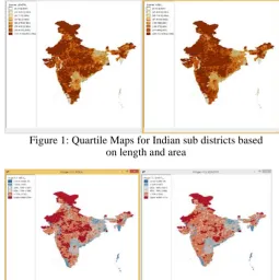
Figure 1 represent the different types of maps for the given datasets. In figure 1, a quantile map, the sub districts are sorted and grouped in categories with equal numbers of observations based on length and area. Figure 2 represents box map. Here the Indian sub districts are classified into six different classes. First four are basic classifiers, the next quartile represent the highest degree of low values, and the last quartile represents highest degree of high vales in the sub districts area.

Figure 1: Quartile Maps for Indian sub districts based on length and area

Figure 2: Box Maps for Indian sub districts based on length and area

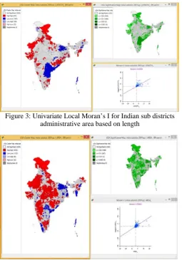
districts are therefore those that contribute significantly to a positive global spatial autocorrelation outcome, while paler colors contribute significantly to a negative autocorrelation outcome. Three different types of maps and graphs are produced here called a significance map, a cluster map and a Moran scatter plot. In this cluster map is the most powerful map which is given. This map provides essentially the same information as the significance map, but with the significant sub districts colure coded by type of spatial autocorrelation. The combination of the Cluster Map and the Significance Map allows us to see which sub districts are contributing most strongly to the Indian administrative scenario and in which direction.

Figure 3: Univariate Local Moran’s I for Indian sub districts administrative area based on length

Figure 4: Univariate Local Moran’s I for Indian sub districts administrative area based on area

Figures 5 represent the Bivariate Local Moran’s I. All the three graphs which is discussed in local Maran’s I are generated in this type too, except that they pertain to a bivariate measure of local spatial autocorrelation. The bivariate LISA is a straightforward extension of the LISA functionality to two different variables, in our study we used one for the length and another for the area of sub districts of Indian administrative area.

Figure 6 and 7 represents local Moran’s I with EB rate variables. In this map also three graphs are generated as for the Univariate LISA, except that they pertain to a measure of local spatial autocorrelation computed for EB rates.

Figure 5: Bivariate Local Moran’s I for Indian sub districts administrative area

Figure 6: Local Moran’s I with EB rate for Indian sub districts administrative area based on length

Figure 7: Local Moran’s I with EB rate for Indian sub districts administrative area based on area Figure 8 represents local G Statistics map showing clusters of significant high and low values in the sub districts and the significance map indicating the p-values for each polygon in the sub districts of Indian administrative area.

The following tables discussed about various SaTScan tool results which we have gotten from Indian sub districts administrative area. Table 1 gives summary of data results obtained. Table 2 and 3 provides the cluster details obtained from SaTScan tool for the given Indian administrative datasets. Table 4 provides the various parameter settings such as analysis, inference and other output.

Table 1: Summary of the results using SaTScan

SUMMARY OF DATA

Study period...: 2000/1/1 to 2015/12/31

Number of locations...: 5463

Total population...: 1210622

Total number of cases...: 506000

Annual cases / 100000...: 2612.2 Table 2: Clusters analysis results using SaTScan Table 3: Clusters analysis results using SaTScan

Table 4: Analysis, Inference and Output analysis results using

SaTScan

VI. CONCLUSION

In this paper, experiments on sub districts of Indian administrative data sets are conducted to analyze the various statistical methodologies by using Geoda and SaTScan tools. Here, the data set contains five attributes and 5470 attributes.

From the above results it’s proved that GeoDa consists of an interactive environment that combines maps with statistical graphics, using the technology of dynamically linked windows. Along with that Geoda mapping functionality contains the different graphs such as histogram, box plot, scatterplot and implements brushing for both maps and statistical plots. In addition, GeoDa contains a Moran scatterplot and LISA maps, both univariate as well as bivariate. Whereas SatScan method may uncover clusters that are not relevant to the exposure. At present, SaTScan does not operate within popular GIS applications such as ArcGIS. Datasets have to be exported for SaTScan, and results have to be linked back to the GIS data for visualization.

Finally it is concluded that GeoDA happens to be the best among the tools in predicting effective and efficient statistical results. It is amazing to note the drawbacks of SaTScan clearly thru our results which will certainly help the future researchers also.

VII. ACKNOWLEDGMENT

One of the authors K.Balaji acknowledges Rayalaseema University, Kurnool, Andhra Pradesh, India and Surana College PG Departments, Bangalore, Karnataka, India for providing the facilities for carrying out the research work.

Analysis

Type of Analysis : Purely Spatial

Probability Model : Discrete Poisson

Scan for Areas with : High Rates

Spatial Window

Window Shape : Circular

Isotonic Scan : No

Inference

P-Value Reporting : Default Combination

Number of Replications : 999

Adjusting for More Likely Clusters : No

Spatial Output

Report Hierarchical Clusters : Yes

Report Gini Optimized Cluster Collection : Yes

Report Gini Index Cluster Coefficents : No

Restrict Reporting to Smaller Clusters : No

Run Options

Processer Usage : All Available Proccessors

Suppress Warnings : No

Logging Analysis : Yes

CLUSTERS DETECTED

1.Location IDs included.: location3975, location3987, location3980, location3982, location3979, location3983, location3053, location3981

Overlap with clusters.: No Overlap

Coordinates / radius..: (11.925267 N, 79.832070 E) / 25.88 km

Gini Cluster...: Yes

Population...: 390

Number of cases...: 5015

Expected cases...: 162.86

Annual cases / 100000.: 80439.3

Observed / expected...: 30.79

Relative risk...: 31.09

Log likelihood ratio..: 12359.088039

P-value...: < 0.00000000000000001

2.Location IDs included.: location4734, location4732, location4735, location4602, location4739,location4738, location4736, location4765, location4731, location4737, location4733, location4754, location4740, location4614, location4604,location4730, location4759,location4601, location4755, location4753, location4766, location4760, location4726, location4756, location4603, location4758, location4742,location4757, location4600,location4769, location4767, location4615, location4728, location4768, location4729, location4752, location4741, location4770, location4727,location4660, location5040,location4745, location4725, location4751, location4616, location4746

Overlap with clusters.: 8

Coordinates/radius:(21.714451N, 83.839124E)/ 77.87km

Gini Cluster...: Yes

Population...: 7184

Number of cases...: 4309

Expected cases...: 3002.50

Annual cases / 100000.: 3748.9

Observed / expected...: 1.44

Relative risk...: 1.44

Log likelihood ratio..: 251.870882

VIII. REFERENCES

[1] Electronic Publication, “Spatial Data Mining”, Techipedia article.

[2] Dhillipan, Dhakshnamurthy and Shanmugam, “Spatial Data Mining Techniques”, International journal for research in emerging science and technology, volume-3, special issue-1, 2016.

[3] Ranu Sahu and Raghvendra Kumar, “Privacy Preservation in Spatial Database”, International Journal of Research, p-ISSN: 2348-6848, e-p-ISSN: 2348-795, Volume 03 Issue 09, May 2016.

[4] Shashi Shekhar and Sanjay Chawla, “Spatial Databases: A Tour”, Pearson Education, 2003.

[5] Anselin, “SpaceStat, a Software Program for Analysis of Spatial Data”, Santa Barbara, CA: National Center for Geographic Information and Analysis (NCGIA), University of California, 1992.

[6] Martin Kulldorff, “SaTScan user guide for version 9.4”, www.satscan.org, 2005.

[7] Luc Anselin, Ibnu Syabri, Youngihn Kho,”An introduction to spatial data analysis”, Geographical Analysis, Wiley Online Library, 2005.

[8] Luc Anselin,”GeoDa 0.9 user’s guide”, Centre for spatially integrated social science, Department of Agricultural and Consumer Economics, University of Illinois, 2003.

[9] Anselin,”GeoDa 0.95i Release Notes”, Spatial Analysis Laboratory, Department of Agricultural and Consumer Economics, University of Illinois.

[10] Srimani P.K and K.Balaji, “Performance of Different Statistical Techniques on Indian Administrative Data by Using GeoDa”, International Journal of Innovative Research in Computer and Communication Engineering, Vol. 5, Issue 1, January 2017.

[11] Esra Ozdenerol, Bryan L Williams, Su Young Kang and Melina S Magsumbol, “Comparison of spatial scan statistic and spatial filtering in estimating low birth weight clusters”, International journal of health Geographics, 2005.