Instance segmentation and material classification in X-ray computed tomography

Boston University

OpenBU http://open.bu.edu

Theses & Dissertations Boston University Theses & Dissertations

2019

Instance segmentation and

material classification in X-ray

computed tomography

https://hdl.handle.net/2144/36044 Boston University

BOSTON UNIVERSITY COLLEGE OF ENGINEERING

Thesis

INSTANCE SEGMENTATION AND MATERIAL CLASSIFICATION IN X-RAY COMPUTED TOMOGRAPHY

by

BORAN HAO

B.S., Beihang University, 2017

Submitted in partial fulfillment of the requirements for the degree of

Master of Science 2019

© 2019 by BORAN HAO All rights reserved

Approved by

First Reader

David Castañón, Ph.D.

Professor of Electrical and Computer Engineering Professor of Systems Engineering

Second Reader

Pirooz Vakili, Ph.D.

Associate Professor of Mechanical Engineering Associate Professor of Systems Engineering

iv

ACKNOWLEDGMENTS

This thesis is finished under the guidance from my esteemed advisor Prof. Castañón, and the supervision and great support from Prof. Vakili. Our work cannot be achieved without the data science knowledge and help offered by Prof. Prakash Ishwar, Prof. Francesco Orabona and Prof. Ioannis Paschalidis. I sincerely appreciate everyone who trusted and supported me, with my highest respect.

This material is based upon work supported by the U.S. Department of Homeland Security, Science and Technology Directorate, Office of University Programs, under Grant Award 2013-ST-061-ED0001. The views and conclusions contained in this document are those of the authors and should not be interpreted as necessarily representing the official policies, either expressed or implied, of the U.S. Department of Homeland Security.

v

INSTANCE SEGMENTATION AND MATERIAL CLASSIFICATION IN X-RAY COMPUTED TOMOGRAPHY

BORAN HAO ABSTRACT

Over the past thirty years, X-Ray Computed Tomography (CT) has been widely used in security checking due to its high resolution and fully 3-d construction. Designing object segmentation and classification algorithms based on reconstructed CT intensity data will help accurately locate and classify the potential hazardous articles in luggage. Proposal-based deep networks have been successful recently in segmentation and recognition tasks. However, they require large amount of labeled training images, which are hard to obtain in CT research. This thesis develops a non-proposal 3-d instance segmentation and classification structure based on smoothed fully convolutional networks (FCNs), graph-based spatial clustering and ensembling kernel SVMs using volumetric texture features, which can be trained on limited and highly unbalanced CT intensity data. Our structure will not only significantly accelerate the training convergence in FCN, but also efficiently detect and remove the outlier voxels in training data and guarantee the high and stable material classification performance. We demonstrate the performance of our approach on experimental volumetric images of containers obtained using a medical CT scanner.

vi

TABLE OF CONTENTS

ACKNOWLEDGMENTS ... iv

ABSTRACT ... v

TABLE OF CONTENTS ... vi

LIST OF TABLES ... viii

LIST OF FIGURES……… ix

LIST OF ABBREVIATIONS ... x

CHAPTER 1 ... 1

1.1 Problem and thesis statement ... 2

1.2 Dataset and splitting ... 4

CHAPTER 2 ... 6

2.1 Introduction and related work ... 6

2.2 3-d CNN based on patching strategy ... 7

2.2.1 Model design ... 7 2.2.2 Network training ... 12 2.2.3 CNN deficiency ... 13 2.3 Smoothed 3-d FCN ... 14 2.3.1 Model modification ... 14 2.3.2 Slice-wise training ... 18 2.3.3 Feature maps ... 21 2.4 Segmentation evaluation ... 23 2.5 Conclusion ... 24

vii

CHAPTER 3 ... 25

3.1 Introduction and problem analysis ... 25

3.2 DBSCAN based on connected components ... 27

3.2.1 Algorithm introduction ... 27

3.2.2 Hyperparameters define ... 29

3.3 Implementation and analysis... 31

3.3.1 Performance metric ... 31

3.3.2 Tuning parameters ... 33

3.3.3 Algorithm performance ... 34

3.3.4 Metal artifacts dilemma ... 37

3.4 Outlier detection... 37 3.5 Conclusion ... 39 CHAPTER 4 ... 40 4.1 Introduction ... 40 4.2 Model construction ... 41 4.3 Feature selection ... 43

4.4 Models validation and test ... 46

CHAPTER 5 ... 51

APPENDIX ... 52

REFERENCES……….. 54

viii LIST OF TABLES Table 1.1. ... 4 Table 3.1. ... 34 Table 4.1. ... 42 Table 4.2. ... 47 Table 4.3. ... 47 Table 4.4. ... 50

ix LIST OF FIGURES Figure 1.1 ... 3 Figure 1.2 ... 3 Figure 2.1 ... 9 Figure 2.2 ... 9 Figure 2.3 ... 12 Figure 2.4 ... 14 Figure 2.5 ... 16 Figure 2.6 ... 17 Figure 2.7 ... 19 Figure 2.8 ... 22 Figure 2.9 ... 23 Figure 3.1 ... 29 Figure 3.2 ... 30 Figure 3.3 ... 32 Figure 3.4 ... 35 Figure 3.5 ... 36 Figure 3.6 ... 38 Figure 3.7 ... 38 Figure 4.1 ... 48

x

LIST OF ABBREVIATIONS

AUC ... Area Under Curve CM ... Central Moments CNN ... Convolutional Neural Network CT ... Computed Tomography CV ...Cross Validation DBSCAN ... Density-Based Spatial Clustering of Applications with Noise FCN ... Fully Convolutional Network GLCM ... Grey-Level Co-occurrence Matrix GPU... Graphics Processing Unit GT ... Groundtruth MP ... Maximum Probability OVA ... One vs. All OVO ... One vs. One PD ... Probability of Detection PFA ... Probability of False Alarm QDA ... Quadratic Discriminant Analysis ReLU ... Rectified Linear Unit ROC ... Receiver Operating Characteristic RoI... Region of Interest SVM ... Support Vector Machine

1

CHAPTER 1 Introduction

Computed tomography (CT), aiming at constructing the 3-d images for target objects, uses a collection of projections using X-ray excitation to produce slice information of a 3-d object. Comparing with traditional X-ray multi-angle imaging for article detection, CT has less overlapping of objects in an image, as well as an increased ability to recognize explosives. Therefore, X-ray CT is widely used in security checking, in order to detect, locate and classify the materials in luggage.

Typically, we reconstruct the CT images from signals obtained from optical detectors resulting in grey-level intensity data for different slices of objects, and such intensities are related to the material density information, in terms of average linear attenuation coefficient. In this thesis, we consider CT images obtained using a single CT source spectrum, resulting in a monochromatic estimate of intensity at each voxel. Our goal is to use the reconstructed 3-d intensity data to detect and classify the objects inside, which can be regarded as a 3-d instance segmentation and classification task in computer vision.

In recent years, with the significant development of deep learning theories and Graphics Processing Unit (GPU) computation, instance segmentation algorithms were proposed

based on deep convolutional neural networks (CNNs), such as SDS[1], Mask R-CNN[2] and

PAN[3]. In terms of both segmentation and classification accuracy, these methods

outperform the traditional segmentation and classification algorithms based on image

processing, like watershed transformation[4] and graph partitioning[5]. However, the

2

images, which can be hard to obtain in CT research, due to the difficulty of precisely producing and labeling 3-d training data. This thesis develops a CT instance segmentation and classification framework combining both deep learning and machine learning algorithms, which can be trained and applied on limited, concentrated and label-unbalanced CT image data. We show the effectiveness of these algorithms using training data and test

data from containers scanned using a medical scanner[6].

We will introduce our work in five chapters. In the rest of this chapter, we will briefly review the problem to be solved, the data sets to be used, and the overall structure of our segmentation and classification model. In chapters 2, 3 and 4, we discuss three relatively separated parts in this model, and give implementation results. In chapter 5, we discuss the features and advantages of our model, and propose some possible future work directions.

1.1 Problem and thesis statement

We illustrate our problem in Figure 1.1. In each of our CT images[6] containing 𝑍 numbers

of 𝑋 × 𝑌 slices like Fig 1.1(a), a voxel 𝑣𝑖 with coordinate (𝑧𝑖, 𝑥𝑖, 𝑦𝑖) has an intensity value

𝐼_𝑣𝑖. By manually labeling all the voxels in target objects made from the target materials

(e.g. saline, rubber), we get a groundtruth (GT) image whose one slice is like Fig 1.1(c), which shows the location and material type of each single target object. Our task is a machine learning problem: training a model using CT and GT images, then use this model to segment and classify the target objects in any CT image input, and output the results like GT image.

3

(a) CT input (b) Semantic

segmentation

(c) Instance separation

(d) Instance classification

Fig 1.2: Three main steps in our structure.

Thesis statement: This thesis solves the problem above by three coherent steps: foreground semantic segmentation using smoothed FCN, instance separation using spatial

clustering, and instance classification based on 3-d texture features and kernel SVMs.

An illustration of this solution is shown in Fig 1.2. Given a 3-d CT image input whose one slice is like Fig 1.2(a), we first binary classify each voxel as background or foreground (target) as Fig 1.2(b). Then in Fig 1.2(c), we further separate instances (voxel sets) from

(a) CT image (Z slices) (b) CT image (one slice) (c) GT image (one slice)

Fig 1.1: Illustration of our problem. (a) is one of our reconstructed test CT images with 244 numbers of 512×512 slices, (b) shows one slice in (a), and (c) is the corresponding slice in groundtruth (GT) image which labels the voxels and material types of different target objects.

4

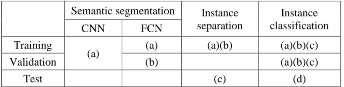
Semantic segmentation _Instance

separation

Instance classification

CNN FCN

Training

(a) (a) (a)(b) (a)(b)(c)

Validation (b) (a)(b)(c)

Test (c) (d)

Table 1.1: Data separation. Image sets: (a) 007~099, (b) 100~109, (c) 160~193, (d) 110~159.

those foreground voxels, which gives the location of target objects. In Fig 1.2(d), we classify the material type for each instance. In this thesis our illustration figures are mostly 2-d, which actually show the 3-d results using one slice.

1.2 Dataset and splitting

Our dataset, known as the ALERT Task Order 4 dataset[6], contains 181 uint-16 CT images

with number 007~193 (a few images invalid) of size 𝑍 × 512 × 512, and each CT image

has a GT image. In this thesis, objects composed of saline, rubber and clay are regarded as target objects. In the dataset, only 1~5 target objects are contained in each CT image, and only no more than 1% voxels are in target objects. Therefore, considering the image/object number and label ratio, this dataset is limited and unbalanced.

Since we only use machine learning methods in our processing structure, dataset should be properly separated to train or test different models. The dataset separation for each section is shown in Table 1.1. We use a test set for at most once to guarantee the independence between the test set and trained model. In deep networks (CNN and FCN) training, we use the validation sets to monitor the training convergence. In instance separation, we use the training images to tune the hyperparameters in the unsupervised

5

clustering model. In instance classification part, we apply k-fold cross validation on training samples. The overall distribution of material labels is balanced among images, thus we do not shuffle the image set before splitting. This will generate some unseen objects in the test set, which can also test the model generalization ability to new objects.

6

CHAPTER 2

Foreground Semantic Segmentation

In this chapter we will discuss our initial problem – labeling all foreground (saline, rubber and clay) voxels in a CT input image, in order to further separate objects from them. We introduce a voxel-wise classification model based on fully convolutional networks (FCNs), and a practical approach to initialize the parameters despite our highly unbalanced class labels. Then, we propose a slice-level smoothed training method to effectively reduce the false-alarm prediction and enhance the segmentation smoothness, meanwhile accelerate the training convergence.

2.1 Introduction and related work

Semantic segmentation is one of the most basic tasks in computer vision research. Comparing with image classification models which only need to give a label to the whole image, a semantic segmentation model predicts the class for each pixel / voxel, without separating different objects. In this section, our goal is to train a binary classification model to classify each voxel as background or foreground.

Traditional methods for binary semantic segmentation, represented by thresholding[7]

methods, graph partitioning methods based on Markov random fields[8], graph multi-way

cut[9], and boundary detection methods[10][11], were widely applied into both 2-d and 3-d

works. Such algorithms can usually be interpreted by image processing techniques and require the use of prior knowledge, and they work efficiently and pertinently for specific

7

GoogLeNet[14]_{, were designed and gained great performance on image classification works}

and competitions. In order to use such classification models to design trainable

segmentation models, fully convolutional networks (FCNs)[15] were proposed, which

modified the final fully-connected layers in traditional CNNs into convolutional layers defined by deep 1×1 kernels. Recently, FCN-based semantic segmentation methods have become the mainstream in 2-d tasks, and in this chapter, we will further illustrate the motivation of applying and improving 3-d FCNs in our work.

2.2 3-d CNN based on patching strategy 2.2.1 Model design

Although theoretically, we can directly implement the 3-d version of 2-d semantic segmentation networks on our dataset, it turns out to be impractical. First, adding one dimension will sharply increase the number of model parameters and training computation complexity, which makes the model hard to train with limited training data; second, though we have billions of voxels as foreground / background training data, they are highly concentrated in a few images with significantly unbalanced foreground / background labels. In a general CT image from our dataset, there are only around 500K foreground voxels among totally 80M~100M voxels, and there exists still around 40M background voxels even if we only consider the ones with non-zero intensity. Such label ratio fluctuates in different images, which often leads a randomly initialized FCN model to give all-background / foreground output after training even with label weights.

8

To solve these problems and implement FCN structures, first we need to generate millions of balanced training samples to initialize the parameters in the corresponding CNN. This motivation inspires us to use a patching training strategy as in [15]. Instead of

only using the intensity 𝐼_𝑣𝑖 to predict 𝑦̂_𝑖 ∈ {0,1} (0 means background, 1 means foreground)

for 𝑣_𝑖, we consider to use the intensities of a 5×5×5 patch around 𝑣_𝑖, a 3rd-order tensor 𝒙_𝒊∈

𝑹𝟓×𝟓×𝟓_{as the feature for 𝑣}

𝑖. Now we wish to use a model ℎ𝜃 ∈ 𝐻 with parameter 𝜃, and

maximum a posteriori (MAP) decision rule to output the label 𝑦̂𝑖 ∈ {0,1} for the central

voxel of this patch:

𝑦̂_𝑖 = ℎ_𝜃(𝒙_𝒊) = 𝑎𝑟𝑔 𝑚𝑎𝑥

𝑦∈{0,1}𝑝̂𝜃(𝑦|𝒙𝒊) (2.1)

where 𝑝̂_𝜃(𝑦|𝒙_𝒊) = 𝑃̂_𝜃(𝑌 = 𝑦|𝑿 = 𝒙_𝒊) is the predicted posterior probability of 𝑦_𝑖 = 0 and

𝑦𝑖 = 1 given 𝒙𝒊, output by the model. The training process of this model is equivalent to

solving the following empirical risk minimization (ERM) problem over 𝑚 patch samples:

𝑚𝑖𝑛

𝜃 ∑ ℓ(𝑝̂𝜃(𝑦|𝒙𝒊), 𝑦𝑖) 𝑚

𝑖=1

, 𝑦𝑖 ∈ {0,1} (2.2)

and we use cross-entropy loss:

ℓ(𝑝̂𝜃(𝑦|𝒙𝒊), 𝑦𝑖) = −𝑦𝑖𝑙𝑜𝑔 (𝑃̂𝜃(𝑌 = 𝑦𝑖|𝑿 = 𝒙𝒊)) − (1 − 𝑦𝑖)𝑙𝑜𝑔 (𝑃̂𝜃(𝑌 = 1 − 𝑦𝑖|𝑿 = 𝒙𝒊)) (2.3) By extracting all patches with foreground labels (including overlapping) and down-sampling background patches (excluding most of patches with all-zero or small intensities), we get 50M of foreground and 50M of background training patches, which is enough to train a relatively deep CNN.

9

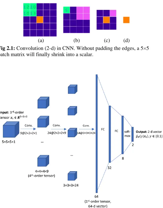
(a) (b) (c) (d)

Fig 2.1: Convolution (2-d) in CNN. Without padding the edges, a 5×5 patch matrix will finally shrink into a scalar.

Fig 2.2: 3-d CNN for patching input. This network, combining 3 convolutional (Conv.) layers and 3 fully-connected (FC) layers, refers

to LeNeT-5[17]. We increase the number of feature maps in the first 3

convolutional layers to extract more detailed features. The activation functions of first 5 layers are Rectified Linear Unit (ReLU) defined in (2.4), and the final layer is a softmax layer defined in (2.7).

1 2 2 0

10

We illustrate the convolution (2-d) in CNN using Fig 2.1. Similar to the convolution in signal processing, a convolution kernel like the 2×2 green area in Fig 2.1 (a) is still like a filter. By sliding the kernel on a 5×5 patch image, at each position we can compute a weighted sum of the 4 pixel values in original image, and the weights are exactly the values in kernel. Using stride 1 for each direction and without padding the edges during sliding, we put each sum at the center of the corresponding position and get a 4×4 convolved image (b). Keep using 2×2 and 3×3 kernels to filter (b) and (c), the 5×5 patch will finally become a scalar at the center. This process can be applied to 3-d patches and kernels.

We design our 6-layer 3-d CNN as ℎ_𝜃 to be trained, as Fig 2.2 shows. In this figure,

we use size 5×5×5×1 to describe this 3rd-order tensor 𝒙𝒊 ∈ 𝑹𝟓×𝟓×𝟓 input, meaning one

channel (grey-level intensity, no RGB) of 5×5×5 patch. We can also regard 𝒙_𝒊 as a 4th

-order tensor here, just like regarding a vector as a ‘matrix’. By letting 9 kernel tensors with size 2×2×2×1 (2×2×2 cube, 1 channel) slide on the input tensor with stride 1 on each direction without padding the edges, the size of input tensor will shrink and end up with 9

channels of 4×4×4 patch – a 4th-order tensor. We express such a convolution method (stride

1, no padding) by 𝐶𝑜𝑛𝑣(𝒙, 𝑲), where 𝒙 is the input tensor to a convolutional layer and

tensor K contains the convolution kernels in this layer. We use Rectified Linear Unit (ReLU)

activation function to further make the mapping non-linear:

𝑅𝑒𝐿𝑈(𝑥) = 𝑚𝑎𝑥{0, 𝑥} (2.4)

If 𝒙 is a tensor, taking ReLU simply means changing all negative entries in 𝒙 to 0. By

11

3 layers in Fig 2.2) in our CNN filtering a tensor 𝒙_𝒊𝒋 to 𝒙_𝒊𝒋+𝟏 can be expressed as:

𝒙_𝒊𝒋+𝟏 = 𝑅𝑒𝐿𝑈(𝐶𝑜𝑛𝑣(𝒙_𝒊𝒋, 𝑲_𝒋) + 𝒃_𝒋) (2.5)

where tensor 𝒃𝒋contains the bias terms for all entries in tensor 𝐶𝑜𝑛𝑣(𝒙𝒊

𝒋

, 𝑲𝒋), but only has

a few (number of kernels in 𝑲_𝒋) unique entry values. Keep applying convolutional

operations, finally the patch will shrink into a 1×1×1 scalar with 64 channels, which is just a 64-d vector. We further use this vector to design the fully-connected layers which use

ReLU activation function (the 4th_{, 5}th _{layer in our CNN):}

𝒙_𝒊𝒋+𝟏 = 𝑅𝑒𝐿𝑈(𝑾_𝒋𝒙_𝒊𝒋+ 𝒃_𝒋) (2.6)

where 𝑾_𝒋 ∈ 𝑹𝒔∗𝒕_{and 𝒃}

𝒋 ∈ 𝑹𝒔help to map the 𝒙𝒊

𝒋

∈ 𝑹𝑡_{input to this fully-connected layer}

to 𝒙_𝒊𝒋+𝟏 ∈ 𝑹𝒔, as the output of this layer. The final softmax layer defined by:

𝑠𝑜𝑓𝑡𝑚𝑎𝑥(𝑦|𝒙_𝒊𝒋, 𝒘_𝒋𝟎, 𝒘𝟏_𝒋, 𝒃_𝒋𝟎, 𝒃_𝒋𝟏) = 𝑒 𝒘_𝒋𝒚𝒙_𝒊𝒋+𝒃_𝒋𝒚 ∑ 𝑒𝒘𝒋𝒌𝒙𝒊 𝒋 +𝒃_𝒋𝒌 𝑘∈{0,1} , 𝑦 ∈ {0,1} (2.7)

is actually also a fully-connected layer using softmax activation function, which will map

the input vector 𝒙_𝒊𝒋 to 2 scalars which are the foreground/background posterior probability

𝑝̂_𝜃 we need to compute the loss. Now in this model, values in convolution kernel tensors

𝑲 (9×2×2×2×1+24×2×2×2×9+64×3×3×3×24=43272), fully-connected layer weight

vectors 𝑾(64×32+32×8+8×2=2320)and bias terms 𝒃(9+24+64+32+8+2=139)compose

the 45731 parameters to be trained. According to agnostic PAC learning theory[16], a rule

12

samples 𝑚 at least 20 times of parameters in model, thus using 100M of patches gives us

enough confidence to estimate the parameters accurately.

When all the patches are classified, the image is segmented. Notice that in convolution since we do not pad the edges for even the edge patches in CT input, the size of segmentation output will be smaller than CT input, and we simply give the unclassified voxels background labels because no objects are put in those edge positons.

2.2.2 Network training

We split 100M of patches into validation set (1M) and training set (99M). Since we use

uint-16 CT image, the intensity values are divided by 216− 1 as a normalization step, to

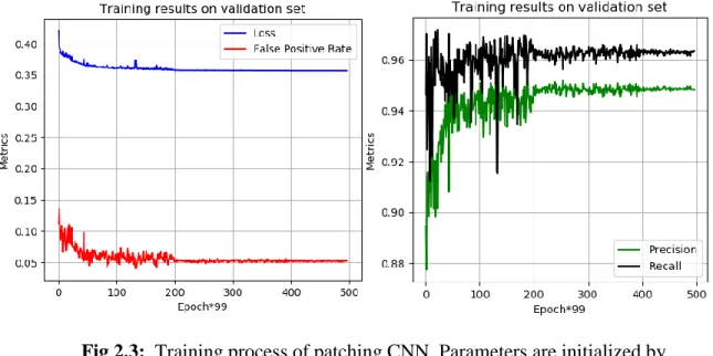
Fig 2.3: Training process of patching CNN. Parameters are initialized by

truncated (3σ) standard Gaussian random variables. In mini-batch gradient

descent, each mini-batch contains 50 (25 foreground + 25 background) samples, and all 99 million samples will be fed into CNN exactly once in

an epoch. The stepsize for epoch 1~5 are 10−2, 10−2, 10−3, 10−3, 10−4,

and convergence can be confirmed at the end of the 4th _{epoch. No dropout}

13

avoid the gradient explosion in training process. The training setting and results are shown in Fig 2.3, and the metrics (precision, recall and false positive rate, see Appendix) are all calculated from the confusion matrix of predicting all voxels in validation set. We use those metrics on validation set to monitor the training process. When the convergence is observed, we stop the training. Sometimes the loss on validation set may increase after certain iterations, which indicates an overfitting problem, and we need to early-stop the training. Nevertheless, no such overfitting is observed in our implementation.

An important step before each cyclic epoch of training is to completely shuffle all the 99M of training samples, since samples from a certain image usually share certain patterns. Such patterns will seriously influence the convergence since we use mini-batch gradient descent, whose convergence tend to be influenced more by the latest training mini batches. For each epoch, such shuffling takes almost half of the time in training process, but it significantly stabilizes the training convergence.

2.2.3 CNN deficiency

With CNN and enough balanced training data, we already have a model to segment the images patch by patch. However, this strategy is seriously inefficient. Most of the convolution computations are repeated since patches are overlapping. Besides, this training method only considers the local intensities, but abandons global information given by the whole CT image. Fig 2.4 shows the problems in output using the patching model. Most of background voxels (box, cloth, air, etc.) are successfully eliminated. However, although we do not require a perfect segmentation in this stage, here are 2 major problems in CNN

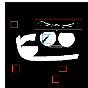
14 (a) CT input

(c) Patching CNN output (b) Ground truth

Fig 2.4: One slice output of trained patching CNN. Failing to remove 2 cans of diet cokes is not a big issue in this section since they have similar intensity information with saline, but small false alarms and segmentation inconsistency should be solved.

output: small false alarm voxels remained (red boxes in (c)), and segmentation inconsistence (blue box in (c), in a diet coke background object). Such inconsistency may

be caused by a general misclassification, or metal artifacts[18] in CT. A metal ball is located

in the blue box in (a), though being successfully classified into background, its disturbance to the surrounding objects remains. To solve such problems, we modify our structure and continue training, using our smoothed FCN model.

2.3 Smoothed 3-d FCN 2.3.1 Model modification

To solve the problems in previous CNN and make use of global information, we further consider the following optimization problem:

15 𝑚𝑖𝑛 𝜃 ∑ 𝐶𝑖ℓ(𝑝̂𝜃(𝑦|𝒙𝒊), 𝑦𝑖) 𝑚 𝑖=1 + 𝜆 (∑|𝜓_𝜃(𝒙_𝒊)|𝑝 𝑚 𝑖=1 ) 1 𝑝 (2.8)

Comparing to the ERM problem in (2.2), (2.8) is intuitively like a regularized problem with

sample weights 𝐶_𝑖, though the added term is not technically a regularizer. Basically, now

we define the objective function as two parts: data term loss ∑𝑚_𝑖=1𝐶_𝑖ℓ(𝑝̂_𝜃(𝑦|𝒙_𝒊), 𝑦_𝑖), which

has already been defined in (2.2), and smoothness term loss 𝜆(∑𝑚_𝑖=1|𝜓_𝜃(𝒙_𝒊)|𝑝) 1

𝑝_{, which} measures how ℎ𝜃(𝒙𝒊) different from ℎ𝜃(𝒙𝒋), and 𝒙𝒋 are the feature patches located near

around 𝒙_𝒊 in CT image. Solving this new problem means we wish to slightly increase the

estimation error, to make segmentation globally coherent. We define 𝑝 = 1 since the

empirical observation shows that 𝑙1 norm better eliminates false alarms and makes

convergence faster, and:

𝜓_𝜃(𝒙_𝒊) = 𝑃̂_𝜃(𝑌 = 1|𝑿 = 𝒙_𝒊) − 1

|𝑁_𝒙𝒊| ∑ 𝑃̂𝜃(𝑌 = 1|𝑿 = 𝒙𝒋) 𝒙𝒋∈𝑁_𝒙𝒊

(2.9)

Here 𝑁_𝒙𝒊 is the set containing 𝒙_𝒊 and all 26 patches 𝒙_𝒋 around 𝒙_𝒊, meaning the center voxel

𝑣_𝑗 of 𝒙_𝒋 in CT image is among the 3×3×3 cube centered by 𝒙_𝒊. By also minimizing such

smoothness term, we make the posterior probability given 𝒙_𝒊 output by model as similar as

16

(a) (b) (c)

Fig 2.5: Convolution operations in patching CNN can be shared.

Fig 2.5 shows how to solve the repeated convolution operations. In the prediction for the patches in Fig 2.5(a) and (b), all the values in convolution – original image, red dots in 4×4 patch and green boxes in 3×3 patch – have overlapping parts. If we directly slide the kernels on the whole region as in (c), the individual operations for two 5×5 patches are still the same, but there will be no repeated convolution. This indicates that we can directly slide the trained kernels on the whole CT input to improve the prediction speed.

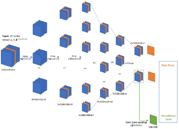
Now we can introduce the smoothed FCN structure shown in Fig 2.6. The predicting process is completely equivalent to the previous patching CNN in Fig 2.2, but the efficiency is greatly enhanced by sharing the convolution operations. This structure can segment any shape of 3-d input, since we only slide convolution kernels on the whole tensor input and take combination of later channels instead of doing any fix-shape tensor

operation. In prediction, similar to 3-d CNN, a 𝑍 × 512 × 512 input tensor will shrink into

a (𝑍 − 4) × 508 × 508 × 64 tensor at the end of convolutional layers, and the previous

channels. If we use Z = 5 slices input, the output is exactly the prediction of central slice.

In training, we can also use a whole CT image as input as long as the system memory is enough, but we need at least 7 coherent slices as input, since we need at least 3 slices of

17

weights in CNN fully-connected layers are still the combination coefficients for the current foreground maps to compute the 3-d smoothness term loss we defined. To get the

smoothness loss for the central slice, we use a 3×3×3 kernel with entries 1

27 to filter the 3×508×508 foreground posterior probability tensor, and a 508×508 matrix (green slice) will be obtained since we pad 0 on edges for each 508×508 slice. Finally, we subtract this

green slice matrix from foreground posterior probability matrix and compute 𝜓𝜃(𝒙𝒊) for

each 𝒙𝒊. Notice that even if we may only have hundreds of tensors to train, we are actually

Fig 2.6: Smoothed FCN structure. The parameters we trained in patching CNN model can be directly used in this vectorized structure. For training, we input 7 layers to get 3 final foreground/background maps, then use the center slice to compute the data-term loss, and use the whole 3 foreground maps to

build the spatial smoothness term defined by 𝜓_𝜃(𝒙_𝒊). After computing the

cross-entropy loss for each of the voxel in final 2 orange maps, sample weights are added to balance label bias and tune the prediction tendency.

18

still training millions of ‘patches’ together in one mini batch, thus the data amount is still enough to make the FCN model learnable.

To train with tensor input, properly setting sample weight parameters 𝐶_𝑖 is extremely

important. The basic motivation is that the label ratio is no longer balanced in slices, and background voxels are far more than foreground voxels. If we keep setting the label weight

for background and foreground 𝐶_𝐵 = 𝐶_𝐹, then mistakenly predicting background voxels

will receive more penalty than foreground voxels, which finally makes more voxels tend to be predicted as background. Therefore, together with the smoothness parameter, we define label weight ratio:

𝑟 = 𝐶𝐹 𝐶𝐵

(2.10)

to solve the label unbalance, and further control the tendency of the model prediction.

2.3.2 Slice-wise training

Considering our computational capability, in smoothed FCN training process, each of our training input is a 7×512×512 tensor. Since lots of slices in CT image contain no target or even background objects, properly selecting the slices to be trained will not only increase our training efficiency, but also decrease the difference of label ratio among the input tensors and help us to stabilize the training process. Therefore, we check the training CT images 7~99, and select 248 non-overlapping tensors as training data. Though we only choose on average 3 tensors from each image, information from 21 slices which contains all background / target objects at least once are used, and these objects appear repeatedly

19

(a)

(b)

(c)

20

in different images. More slices or even overlapping tensors could be used to train, but our selection already gives us good enough results.

Fig 2.7 shows the training process and validation performance. In each epoch, we cyclically feed 248 tensors and the corresponding groundtruth label layers (508×508) into FCN. We initialize the parameters in smoothed FCN using the training result in patching CNN, and fix the gradient descent stepsize as 0.0001. By predicting all the voxels in validation images, we can still monitor the convergence like we did in CNN. The purpose of this further training is not only removing the false alarms brought by container or metal artifacts, but also padding the segmentation inconsistency in some unavoidable false alarm

like diet coke in Fig 2.4. To remove the false alarms, we can simply use a small 𝑟 to train,

as shown in Fig 2.7 (a). Even without setting smoothness term, the label unbalance will lead to a background prediction tendency. However, the segmentation inconsistency caused by metal artifacts in diet coke and a saline object becomes more serious, and even

after 200 epochs, small false alarm points still exist. Furthermore, setting a larger 𝑟 as

shown in Fig 2.7 (b) to pad the inconsistency will also sharply increase the false positive rate. Nevertheless, by adding a small smoothness parameter in Fig 2.7 (b) to train as in Fig 2.7 (c), the increasing of false positive rate will be prevented. After the smoothed objective function converges, we can observe that small false alarm voxels are efficiently eliminated,

Fig 2.7: Training process and the influence of using different label weight

ratio 𝑟 and smoothing parameter 𝜆. For (a)(b)(c) and (d), we record the FCN

performance on validation set in different epochs, and output the segmentation for the slice in Fig 2.4 using the model after epoch 10 (left) and 200 (right). We use image 100~109 as validation images to evaluate the prediction for each voxel.

21

and the inconsistency is padded. By properly tuning 𝑟 and 𝜆, two opposite tendencies –

eliminating and padding – can be simultaneously achieved. Fig 2.7 (d) shows a better

parameter setting, which increases both 𝑟 and 𝜆. Comparing (d) to (a), even after padding

some background objects inconsistence, the false positive rate in (d) still decreases as much as (a), which also indicates that adding smoothness term efficiently cancels false alarm voxels.

In Fig 2.7 we can also observe that the convergence is accelerated by adding smoothness term. Training without smoothing leads to 200 epochs to roughly observe

convergence, while setting 𝜆 accelerates the convergence within 50 epochs. Notice that it

is unavoidable that some true foreground prediction will be removed while eliminating false alarm, thus the segmentation recall will be influenced. Though such shrinkage of foreground is not obvious, considering maintaining a higher recall in our later detection work, we use an early-stopped model after epoch-2 in Fig 2.7 (d) to output the foreground-background segmentation images to be used in later works.

2.3.3 Feature maps

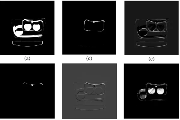
In FCN predicting process, the tensors in hidden layers called feature maps in Fig 2.6 can always be extracted. Those maps can intuitively interpret how FCN extracts features from intensity input. Fig 2.8 shows part of the feature maps in convolution layers. In the first

convolution layer, though the orange layer cannot be located, we use the 2nd layer of 4 to

show feature map, and intensity features are extracted by directly filtering the small intensities as background in Fig 2.8 (a), and locating the position of metal in Fig 2.8 (b). In

22

(a) (c) _(e)

(b) (d) (f)

Fig 2.8: Part of FCN feature maps in first 3 convolution layers ((a)(b)

from 1st, and (c)(d), (e)(f) from 2nd, 3rd). Using the FCN model trained

after 2 epochs with setting in Fig 2.7 (d), these maps are still for the same slice in Fig 2.4.

the second layer, more detailed features are found, basically the edge of objects in Fig 2.8 (d), and some certain background objects like container in Fig 2.8 (c). The third layer can be more detailed and weirder by detecting the boundary in certain direction like Fig 2.8 (e), or showing how gaps caused by metal artifacts can be compensated in Fig 2.8 (f).

Such feature maps reveal the most fascinating characteristic of deep learning. Even if we do not use any prior knowledge in image processing or physics, the model can still learn the most effective features – within our cognition or not – to make reasonable decisions. To some extent, we can say that training a neural network is equivalent to finding the best feature maps, since the last layer is always a simple linear classifier, and the quality of

23

(a) CT input (b) Thresholding (c) Smoothed FCN (d) Groundtruth

Fig 2.9: Smoothed FCN and thresholding segmentation comparison. Even

under strong metal artifacts, the segmentation consistency and accuracy can still be guaranteed.

features decides the quality of decision. In many proposal-based instance segmentation

networks like Fast R-CNN[20], selecting proper feature maps is the initial step before

extracting region proposals.

2.4 Segmentation evaluation

The validation recall in patching CNN and FCN are similar, while the validation precision of FCN (around 40%) is much lower than CNN. This indicates that through our foreground segmentation network, most of the voxels from target objects are detected, but there are still almost equal number of false alarm voxels from background objects which are failed to be removed. This can be explained by dataset unbalance, since although we select patches with higher intensity, they are still a minority of the background voxels with high intensity values.

The great difference between the segmentation performance between FCN and simple thresholding methods can be observed in Fig 2.9. Although the intensity threshold 1000~2000 we set is already extremely strict, background voxels from container and metal

24

artifacts cannot be eliminated. In addition, target voxels are mistakenly removed from rubber sheet. Nevertheless, our smoothed FCN perfectly solves both problem and gives the segmentation almost identical to groundtruth. Indeed, simple methods can still give seemingly good voxel classification performance metrics, but the true advantage of using FCN can never be simply evaluated by those small metric differences.

2.5 Conclusion

In this chapter, we introduced and solved the foreground-background semantic segmentation task. The segmentation model and training method we designed is an improvement of original FCN to fit our 3-d task. First, by using the parameters initialized by a carefully trained patching CNN model, we stabilized the parameters in FCN training process within a reasonable range, to avoid the all-background / foreground prediction or the sharp fluctuating of parameters brought by directly training FCN initialized by random parameters. Second, by adding the 3-d smoothness term in FCN loss function, the global information in CT image was used, which significantly solved the segmentation inconsistency caused by metal artifacts and accelerated the convergence. Our idea can be applied to any 2-d / 3-d semantic segmentation work based on FCNs and modified by adding pooling / deconvolutional layers.

25

CHAPTER 3 Instance Separation

This chapter introduces a non-proposal instance separation approach to further separate the foreground voxels in our previous semantic segmentation work into single objects. Based on the specific properties of CT images and target objects, such a graph-based clustering algorithm accurately separates the instances and removes the false alarm voxels as noise. Furthermore, we propose an outlier detection approach based on this clustering algorithm, which will significantly improve the material classification performance. We use the validation results to show how parameter setting influences the separation process, and give analysis for the metal artifact influence in clustering.

3.1 Introduction and problem analysis

In our task, instance separation is more like an object detection work. Even if objects are spatially adjacent in CT image and foreground segmentation, now we should figure out their independency and separate them as individual instances.

The latest methods for such task can be roughly classified into 2 classes: proposal-based methods, and non-proposal methods. Proposal-proposal-based models, represented by fast

R-CNN[20], faster R-CNN[19], use FCN feature maps and basic detection methods like

selective search[21] to find proposal regions of interest (RoIs), in order to further compute

the confidence of RoIs containing objects and make classification, or train the network. Comparing to the complex structure of proposal-based constructions, non-proposal methods are structurally simpler but more elegant. By carefully defining loss functions,

26

mean-shift algorithm[22] _{and Gaussian blurring mean-shift algorithm}[23] _{are used to cluster}

voxels in embedding space, and voxels from a same object tend to shift into the same group.

YOLO[24] was designed in a similar way as faster R-CNN, but it pre-divides an image into

grids and trains a regression model to tune the bounding box shapes.

By analyzing our task and CT objects, we will find the following properties: (1) Local stability

Our target objects (saline, rubber, clay) have relatively stable intensity features (local mean, variance) in an object, and this is rare in other segmentation tasks. We may want to segment a car in 2-d traffic image, but obviously the car wheels have different color and texture features from its metal frame.

(2) Non – overlapping

In 2-d images, if we want to localize and segment each individual in crowd, we need to consider the body part obscured by others and try our best to recover the original position. Nevertheless, in CT image each voxel reflects a unique position in 3-d space, and nothing can be obscured by others.

(3) Data scarcity

Directly implementing proposal-based deep networks to our separation problem is not practical, since we only have about 100 training images with no more than 300 repeated groundtruth objects.

Considering the characteristics above, we introduce a non-proposal approach to separate instances. This idea is based on a density-based spatial clustering of applications

27 to better fit our task.

3.2 DBSCAN based on connected components 3.2.1 Algorithm introduction

Rather than using the concepts in original DBSCAN algorithm, we use a graph to introduce our modified DBSCAN and how we apply it to our object separation work. In a single 𝑍 × 512 × 512 CT image, using segmented foreground voxels 𝑣_𝑖 ∈ ℱ with coordinates

(𝑧_𝑖, 𝑥_𝑖, 𝑦_𝑖) and the corresponding intensity values 𝐼_𝑣𝑖, we can define an undirected graph

𝒢 = (𝑉, 𝐴), where 𝑉 is the node set containing all 𝑣_𝑖 ∈ ℱ , and arc set 𝐴 consists all arcs 𝑎_𝑖𝑗 = {𝑣_𝑖, 𝑣_𝑗} satisfying 𝐷(𝑣_𝑖, 𝑣_𝑗) = 1. We will discuss how to define 𝐷(𝑣_𝑖, 𝑣_𝑗) later, and now we can temporarily regard 𝐷(𝑣_𝑖, 𝑣_𝑗) = 1 as ‘𝑣_𝑖, 𝑣_𝑗 are close and similar enough’. Define 𝒜(𝑣𝑖) = {𝑣𝑗 ∈ 𝑉|(𝑣𝑖, 𝑣𝑗) ∈ 𝐴} as the adjacency list of 𝑣𝑖. Given 𝒢 and integer 𝑁_𝑚𝑖𝑛> 0, let us first give the Algorithm 3.1.

Algorithm 3.1 DBSCAN based on connected components

Initialize 𝑐(𝑣𝑖) = 0, 𝑙(𝑣𝑖) = 0, ∀𝑣𝑖 ∈ 𝑉;

for𝑣𝑖∈ 𝑉:

𝑐(𝑣𝑖) = 1if|𝒜(𝑣𝑖)| ≥ 𝑁𝑚𝑖𝑛;

end

build subgraph 𝒢𝑐 from 𝒢, by removing 𝑣𝑖 with 𝑐(𝑣𝑖) = 0 and related arcs;

In 𝒢𝑐, find maximal connected components 𝑀1, . . . , 𝑀𝑘; 𝑙(𝑣) = 𝑘 for all 𝑣 ∈ 𝑀𝑘:

for 𝑝= 1,2…, 𝑘:

build subgraph 𝒢𝑝 from 𝒢, by removing 𝑣𝑖 with 𝑙(𝑣𝑖) ∉ {0, 𝑝} and related arcs;

In 𝒢𝑝, find maximal connected component 𝑀𝑝 containing any 𝑣: 𝑙(𝑣) = 𝑝;

𝑙(𝑣) = 𝑝for all 𝑣 in 𝑀𝑝;

end

28

In this algorithm, finding maximal connected components can be finished[26] _in

𝑂(𝑚𝑎𝑥 {|𝑉|, |𝐴|}) using depth first search, and the overall worst-case time complexity is 𝑂(|𝑉|2_{), same as original DBSCAN.}

Basically, we wish to label each voxel 𝑣_𝑖 as 𝑙(𝑣_𝑖) = 𝑘, then 𝑆_𝑘 = {𝑣_𝑖|𝑙(𝑣_𝑖) = 𝑘 > 0}

will be cluster 𝑘, i.e. separated object 𝑘 in an image. Voxels having at least 𝑁_𝑚𝑖𝑛 of

neighbors in graph are called core points, which will be labeled as 𝑐(𝑣𝑖) = 1 in Algorithm

3.1. Fig 3.1 intuitively shows how this algorithm works. The two obvious advantages of such clustering method can be observed through this process. First, the objects that are ‘weakly’ connected will be still separated. A voxel must have enough adjacent similar voxels in order to become a core point and connect two objects into one, instead of simple

adjacency (𝑁_𝑚𝑖𝑛 = 1). Second, those voxels still have cluster label 0 after the algorithm

will be removed as noise, which will leave us the most stable and coherent voxels for classification. This feature is extremely important to our later outlier detection work.

The output of this algorithm is highly sensitive to the definition of 𝐷 and 𝑁_𝑚𝑖𝑛. If we

set 𝑁𝑚𝑖𝑛 = 2 in Fig 3.1, then separation will fail; if we only use the spatial distance to

define 𝐷, noise voxels will be included, and separation failure is extremely possible since

we have many objects spatially adjacent to others extensively. That is the basic motivation

why we need to carefully define and tune 𝐷 and 𝑁_𝑚𝑖𝑛. After finishing the clustering, we

finally remove the clusters 𝑆𝑘 if |𝑆𝑘| is less than a minimum object size of 𝜀 voxels, since

29

3.2.2 Hyperparameters define

As we analyzed earlier, since there is no overlapping in 3-d image, all voxels in one object

𝑣𝑖 ∈ 𝑆 shall be spatially adjacent to at least one other 𝑣𝑗 ∈ 𝑆, except for the influence of

noise. We define 𝐷(∙,∙) as following:

(a) (b) (c) (d)

(e) (f) (g) (h)

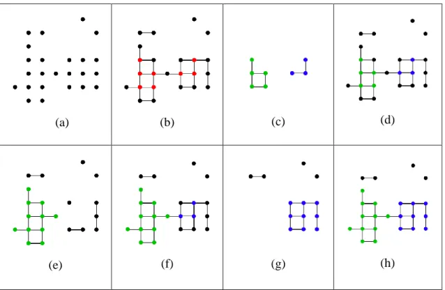
Fig 3.1: A 2-d illustration for Algorithm 3.1. 3-d cases share the same idea.

By calculating the 𝐷(∙,∙) between segmented foreground voxels in (a), we

define the graph in (b) with red core points who have at least 𝑁𝑚𝑖𝑛 = 3

neighbors. We label these core points as blue and green in subgraph (c) by finding the maximal connected components. Next in (e)(g), we again find maximal connected components in the subgraph (d)(f) generated by eliminating blue or green nodes, in order to label the rest of nodes in (d). In final result (h), 2 clusters (objects) are separated, and the remaining unlabeled voxels are noise. Notice that the label of some points may be influenced by the sequence of (e) and (g), thus the algorithm may not be robust in some cases.

30

𝐷(𝑣𝑖, 𝑣𝑗) = 𝟏 [(‖𝑣𝑖− 𝑣𝑗‖₂≤ 𝜖𝑑) ∩ (|𝐼̅𝑣𝑖− 𝐼̅𝑣𝑗| ≤ 𝜖𝜇) ∩ (|𝑉𝑎𝑟̅̅̅̅̅𝑣𝑖− 𝑉𝑎𝑟̅̅̅̅̅𝑣𝑗| ≤ 𝜖𝑣𝑎𝑟)] (3.1) where the local mean:

𝐼̅𝑣𝑖 = 𝐸[{𝐼𝑣𝑘|‖𝑣𝑖 − 𝑣𝑘‖2 ≤ √3 , 𝑣𝑘 ∈ ℱ}] (3.2) and local variance:

𝑉𝑎𝑟 ̅̅̅̅̅_𝑣

𝑖 = 𝑉𝑎𝑟[{𝐼𝑣𝑘|‖𝑣𝑖 − 𝑣𝑘‖2 ≤ √3}] (3.3) Basically, this setting of 𝐷(∙,∙) claims that if arc (𝑣_𝑖, 𝑣_𝑗) exists in 𝒢, 𝑣_𝑗 should be

spatially located inside the 𝜖𝑑-ball centered by 𝑣𝑖, and have similar local intensity mean

and variance to 𝑣_𝑖. Since the intensity values of an object are distributed over a range, taking local mean will further reduce the intensity difference in a same object. Roughly speaking, the intensity values of saline objects are between 1000~1200, while rubber intensities are between 1200~1600, and clay intensities are over 1500. Furthermore, we wish to use local variance in case some adjacent objects share the similar mean. A purpose of using variance is detecting the object boundary, as shown in Fig 3.2. Recall that 𝑉𝑎𝑟(𝑋) = 𝐸[𝑋2] − (𝐸[𝑋])2_{, thus both mean and variance computation can be finished}

Fig 3.2: Local variance helps us to find the boundary. Generally, a target object should have small local variance shock.

31

in parallel using convolution and matrix operations on GPU.

Apart from defining DBSCAN using graph rather than the original concepts, we also

make the parameter setting more flexible by defining 𝐷(∙,∙) to make the structure fit any

adjacency criterion. As long as we fix the hyperparameters above, we can run the algorithm on segmented images to detect objects.

3.3 Implementation and analysis 3.3.1 Performance metric

Now we are no longer solving a voxel classification problem, so we need to redefine performance metrics to evaluate the clustering performance and tune the parameters. In

ground truth image we have ground truth voxel set 𝐿 for a target object, while in clustering

results we have voxel set 𝑆 for a segment. For any 𝐿 and 𝑆 in a same image, we say ground

truth object 𝐿 is detected by segment 𝑆, if both:

𝑃𝑟𝑒𝑐𝑖𝑠𝑖𝑜𝑛(𝐿, 𝑆) =|𝐿 ∩ 𝑆|

|𝑆| ≥ 𝓅 (3.4) and

𝑅𝑒𝑐𝑎𝑙𝑙(𝐿, 𝑆) =|𝐿 ∩ 𝑆|

|𝐿| ≥ 𝓇 (3.5)

and we say 𝑆 is a hitting segment. It is hard to guarantee a perfect detection, thus a widely

used standard[6] is 𝓅 = 𝓇 = 0.5 for bulk objects, and 𝓅 = 𝓇 = 0.1 for sheet objects, since

32

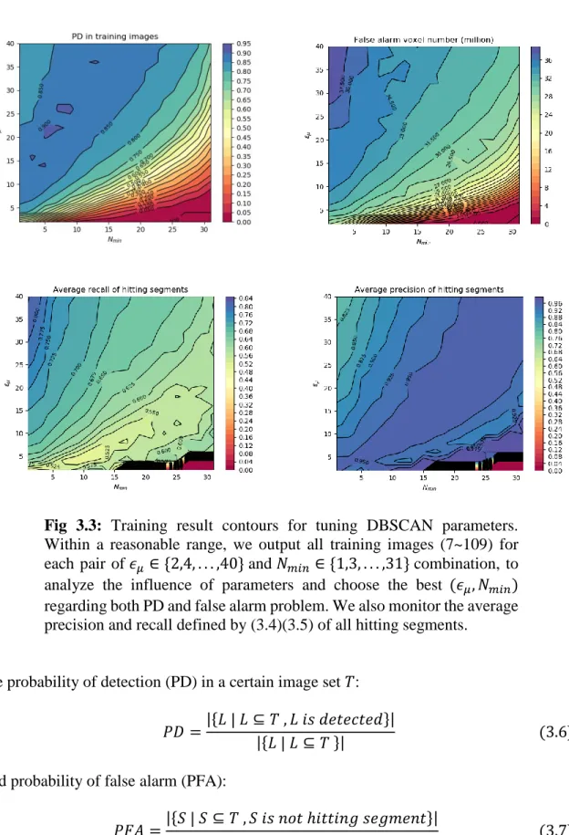
Fig 3.3: Training result contours for tuning DBSCAN parameters. Within a reasonable range, we output all training images (7~109) for each pair of 𝜖_𝜇 ∈ {2,4, . . . ,40} and 𝑁_𝑚𝑖𝑛 ∈ {1,3, . . . ,31} combination, to

analyze the influence of parameters and choose the best (𝜖𝜇, 𝑁𝑚𝑖𝑛)

regarding both PD and false alarm problem. We also monitor the average precision and recall defined by (3.4)(3.5) of all hitting segments.

the probability of detection (PD) in a certain image set 𝑇:

𝑃𝐷 =|{𝐿 | 𝐿 ⊆ 𝑇 , 𝐿 𝑖𝑠 𝑑𝑒𝑡𝑒𝑐𝑡𝑒𝑑}|

|{𝐿 | 𝐿 ⊆ 𝑇 }| (3.6) and probability of false alarm (PFA):

𝑃𝐹𝐴 = |{𝑆 | 𝑆 ⊆ 𝑇 , 𝑆 𝑖𝑠 𝑛𝑜𝑡 ℎ𝑖𝑡𝑡𝑖𝑛𝑔 𝑠𝑒𝑔𝑚𝑒𝑛𝑡}|

33

Like recall, PD reflects how many target objects are successfully detected. PFA shows the

false alarm detection number comparing to the background object (e.g. food) number[6].

Since background object number is fixed, PFA can be even greater than 1 if the algorithm is performing poorly.

3.3.2 Tuning parameters

Though in the definition of modified DBSCAN we have many hyperparameters to tune, we fix some of them by using a reasonable setting. First, we fix the minimum object size 𝜀 = 3600, which is reasonably small and will eliminate most of the micro clusters. By

fixing 𝜖𝑑 = 2.01, we only consider at most 32 nearest voxels around 𝑣𝑖 to further compare

the local mean and variance. In addition, we use local variance to roughly detect the boundary, thus variance difference in the internal region of an object shall not influence

the clustering too much. We set 𝜖𝑣𝑎𝑟 = 20000, then now 𝜖𝜇 and 𝑁𝑚𝑖𝑛 are the two

parameters we need to tune. For each pair of (𝜖_𝜇, 𝑁_𝑚𝑖𝑛), we output all the training images

007~109, and then compute performance metrics for this training image set 𝑇.

The contour in Fig 3.3 Shows the training results. In PD contour, in order to maintain

a high PD, if we increase 𝑁_𝑚𝑖𝑛 – meaning using a stricter standard to choose core points –

then we must also increase 𝜖_𝜇, which relaxes the requirement for forming an arc in 𝒢.

Unlike the overall symmetric trend in PD contour, the false alarm voxel number sharply

decreases if we use large 𝑁_𝑚𝑖𝑛 and smaller 𝜖_𝜇, since such setting tends to cause fewer core

34

guarantee a segment detects a ground truth target object, both precision and recall defined by (3.4)(3.5) shall be sufficiently high, thus we also use the average precision and recall of hitting segments to help tune parameters. In average hitting segment precision contour, precision is high for most of parameters, since DBSCAN finds the most coherent voxels with stable intensity. If a parameter setting causes a low average precision, we should consider that lots of objects are merged in outputs. Also, segments are generally shrunk inside the groundtruth, so the average recall turns to be low.

3.3.3 Algorithm performance

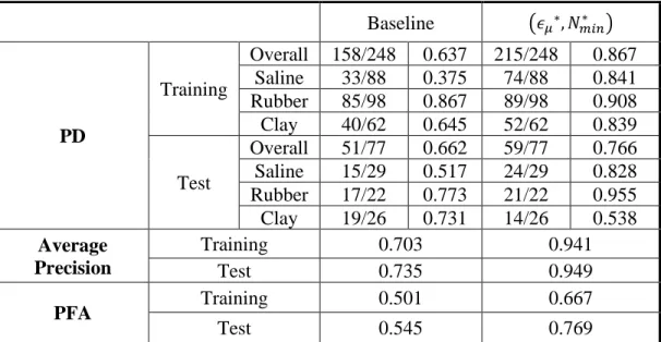
By considering all the four elements, we choose the best parameter combination (𝜖𝜇∗, 𝑁𝑚𝑖𝑛∗ ) = (22,13), and test the detection performance on image 160~193. We set a

baseline performance by using 𝜖_𝜇 = 𝜖_𝑣𝑎𝑟 = ∞ and 𝑁_𝑚𝑖𝑛= 1, which is the simplest case

of only considering the spatial adjacency. The training and test performance are shown in

Baseline (𝜖𝜇∗, 𝑁𝑚𝑖𝑛∗ ) PD Training Overall 158/248 0.637 215/248 0.867 Saline 33/88 0.375 74/88 0.841 Rubber 85/98 0.867 89/98 0.908 Clay 40/62 0.645 52/62 0.839 Test Overall 51/77 0.662 59/77 0.766 Saline 15/29 0.517 24/29 0.828 Rubber 17/22 0.773 21/22 0.955 Clay 19/26 0.731 14/26 0.538 Average Precision Training 0.703 0.941 Test 0.735 0.949 PFA Training 0.501 0.667 Test 0.545 0.769

35

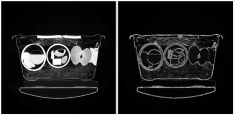
(a) (b) (c)

(d) (e) (f)

Fig 3.4: Separation performance. The segmented foreground voxels in (a) and (d) are successfully separated into objects in (b) and (e), even if the objects are closely attached, or have the circle shapes. (c)(f) are the corresponding ground truth slices.

Table 3.1. Comparing to baseline performance, the overall PD and average precision of hitting segments are greatly increased. Through our observation, the PD of clay in test set is limited due to the serious metal artifacts around clay objects in certain images, which will break clay into pieces and fail to satisfy (3.5). Since these pieces become false alarms, the corresponding PFA gets higher. In this case, the baseline strategy using the weakest adjacency will prevent such breaking, though with a price of merging lots of objects. Analyzing PFA, around 70% is far away from our final 10% goal, and we need to further eliminate them in classification part.

Fig 3.4 shows the effectiveness of using our spatial clustering. Although the adjacent objects like the saline bag and clay sheets in Fig 3.4 (a) are attached extensively in CT foreground segmentation, we can still accurately separate them. For some circle shaped

36

voxels like the clay shell in Fig 3.4 (f), which is known to be hard to cluster using

k-means[27], we can still perfectly divide them with our spatial clustering algorithm, avoiding

more expensive techniques such as spectral clustering[28] and decomposition of large graph

Laplacian matrices.

(a) (b) (c)

(d) (e) (f)

Fig 3.5: Metal effect on DBSCAN. In CT input (a), the strong metal artifacts cause both rubber sheet intensity inconsistency (blue box in (b)) and the intensity merge of clay (between 2 rubber sheets) and the bottom rubber sheet (red box in (b)), thus in clustering output (c), rubber sheet breaks into two pieces and also fails to separate from clay in the middle respectively due to the lack and surplus of core point. Nevertheless, in input (d) metal artifacts are hindered by a rubber sheet, thus clustering result in (f) is good.

37

3.3.4 Metal artifacts dilemma

Although we have observed and partly solved the metal artifacts in foreground segmentation part, the existence of metal artifacts has heavy influence on DBSCAN. Most of failures in separating adjacent objects of different subtype are caused by the nearby metal. Metal has two main opposite effects: makes nearby object intensity locally inconsistent, and changes the adjacent intensities from different objects into a similar range, as shown in Fig 3.5. These two problems – break and merge – cannot be solved simultaneously by tuning parameters in DBSCAN, which becomes the biggest constraint

of our algorithm performance. Notice that although we do clustering in3-d space, strong

metal effect like Fig 3.5 (a) will make the algorithm fail to find core points in other slices to get a detour and connect those rubber sheet pieces in graph.

3.4 Outlier detection

A significant characteristic in our instance segmentation results in Table 3.1 is that the average precision of hitting segments is very high, and the reason for this can be cleverly applied to detect and remove the outlier voxels in training images.

As we can see in Fig 3.6, the ground truth labels are imperfect for 2 main reasons: the boundary of groundtruth object label is not reliable, and there could be holes or gaps inside original objects, which are not indicated in groundtruth. However, the ideal CT intensity shall indicate the material density information, and it does not make any sense if lots of voxels with intensity 0 or under 1000 exist in a clay object. Basically, we can use complex thresholding and prior knowledge to roughly remove them, which could be an inaccurate

38

approach and turn a machine learning problem into image processing. Nevertheless, observing the same object detected in (c) using our algorithm, the object boundary is shrunk, and the unreliable voxels are eliminated as noise in DBSCAN. This trend can be more obviously observed in the grey-level intensity histogram in Fig 3.7. For the same clay object in Fig 3.6, the original ground truth voxel histogram contains a certain percentage of 0 and low intensities which were purified in the histogram of DBSCAN output. The intensity distribution in our segment becomes more like Gaussian, which indicates the intensity distribution of one kind of clay material, instead of a certain clay object. Based on this feature, we design a simple algorithm to remove the outliers in groundtruth labels:

(a) Groundtruth labels (b) CT input (c) DBSCAN output

Fig 3.7: Grey-level intensity histograms of the clay object in Fig 3.6.

39

If there remains no 𝐿𝑘_𝑖 can detect 𝐿𝑖 anymore, this groundtruth label is not reliable itself,

and we will not use it to train any model. After applying Algorithm 3.2 on the clay object in Fig 3.6, the purified groundtruth label in Fig 3.7 now has almost the same intensity histogram as the segment, since a part of clay material is still clay, with identical density distribution. Further using such stable and reliable intensities to do material classification will greatly increase the generalization ability of models trained.

3.5 Conclusion

In this chapter, we redefined and modified the DBSCAN algorithm, and applied it as a practical non-proposal instance separation tool. By properly tuning the clustering parameters, we further removed the false alarm voxels in semantic segmentation results, and kept the most reliable parts inside an object to potentially guarantee a high classification performance. Although using the segmented foreground voxels for clustering extensively decreases the computational complexity of DBSCAN, down-sampling the CT image and using multi-resolution / supervoxel clustering can be simply implemented and further improve the overall efficiency. The outlier detection trick we proposed can also be applied to any material classification problem, regardless of the initial instance separation goal.

Algorithm 3.2 DBSCAN for groundtruth outlier removal Apply DBSCAN on a groundtruth object voxel set 𝐿𝑖, get clusters 𝐿𝑘𝑖 ⊆ 𝐿𝑖;

40

CHAPTER 4 Instance Classification

This chapter solves our final problem – classify the objects detected by modified DBSCAN. We design and train our kernel SVMs based on central moments and volumetric texture features, and compare our results with other material classification structures in X-ray CT. Finally, we use the whole trained construction to test the test images and entire dataset, to evaluate the overall instance segmentation performance in terms of different materials.

4.1 Introduction

The target of our final step is simple: given a segment voxel set 𝑆, predict if it is saline,

rubber, clay, or background. Most of the background objects shall be eliminated in this step. Different from general image classification works in computer vision, our objects have no fixed sizes, thus we need to extract features from them. Deep networks or models using intensity histogram with large number of bins as features shall not be used because of our limited training set, which requires we keep the number of parameters to be learned small.

Choosing the most informative features is more important than using a smart classifier in traditional machine learning based on small sample set, and some of the features we investigate are texture features. Basically, 3-d texture can be divided into two types: space time texture and volumetric texture. Space time texture regards a 3-d image as a time series of 2-d images, while volumetric texture has no concept of time and can be calculated from

41

3-d tensors. Obviously, volumetric texture fits our task better, and a set of 2-d texture analysis methods can be extended to 3-d. Two types of volumetric texture analysis are usually applied to classification task: matrix-based methods and signal processing methods. For matrix-based methods, a set of statistics based on gray-level co-occurrence

matrix (GLCM)[29] was firstly introduced by Haralick to structurally describe the texture

feature, and this idea was applied to 2-d CT organ tissue classification[30] and 3-d texture

description[31]. Using statistics on co-occurrence matrix captures the spatial dependence,

while a set of run-length statistics[32] _{focus on texture coarseness characteristics. In}

addition, a 3-d gradient image can be obtained through convolution, and statistics on

gray-level gradient co-occurrence matrix (GLGCM)[33] can be used as feature to improve the

GLCM results. Methods based on signal processing use signal transform to implement multi-resolution analysis, and features like energy or entropy can be obtained from the

detail frequency coefficients on subbands. Wavelet[34] _{and ridgelet}[35] _{analysis are used to}

extract the image detail pattern in 2-d slices from CT, which can also be modified to 3-d texture construction.

4.2 Model construction

Since DBSCAN is a parameter-sensitive algorithm, the intensity values in our detected objects are highly coherent and stable. However, the groundtruth labels are not coherent as we analyzed in section 3.4, thus we first use Algorithm 3.2 to remove the outliers inside all groundtruth labels before extracting the training features. For background training and test

42

Background Saline Rubber Clay

Training 499 109 112 65

Test 247 27 27 28

Table 4.1: Training and test sample numbers

𝐿_𝑖 ∩ 𝑆_𝑘 = ∅ , ∀𝐿_𝑖 (4.1) in an image to extract background features. (4.1) means a background instance should have no overlapping with any target objects. For target test set, we directly use the hitting segments in test images to get test features and labels, so the test performance will directly indicate how well the models trained on groundtruth labels can be generalized to our segmented instance prediction. The sample number based on the strategy above is shown in Table 4.1.

For small dataset, Gaussian kernel support vector machines (SVMs) with soft margin[36]

are among the most effective binary classifiers, since using kernelized features will generate non-linear decision boundary in original feature space, and application of soft margin with label weights will solve the linear non-separable problem even in kernel space and remedy the label unbalance. To apply SVMs on multi-classification, two general

approaches are: using generalized hinge loss[37] _{to directly construct loss function for larger}

label space, or reduce the multi-classification problem to binary classification using

One-vs-One (OVO) or One-vs-All (OVA)[38] strategy.

Through Table 4.1, saline, rubber and clay labels are roughly balanced, while we have about 2 times of background instances as target. Therefore, to guarantee the label balance

in training process, under the label space 𝒴 = {0,1,2,3} (for background, saline, rubber and

43 OVA approach, and ℎ_𝑠𝑣𝑚1~2_{, ℎ}

𝑠𝑣𝑚 1~3_{, ℎ}

𝑠𝑣𝑚

2~3 _{for the OVO approach to classify 3 subtypes. We}

make the following decision 𝑦̂ for given 𝒙: if ℎ_𝑠𝑣𝑚0~{123}(𝒙) = 0, 𝑦̂ = 0, else:

𝑦̂ = ℎ_𝑠𝑣𝑚(𝒙) = 𝑎𝑟𝑔 𝑚𝑎𝑥 𝑘∈1,2,3∑ ∑ 𝑃𝑠𝑣𝑚 𝑖~𝑗_{(𝑌 = 𝑘|𝑿 = 𝒙)} 3 𝑗=𝑖+1 2 𝑖=1 (4.2) where 𝑃_𝑠𝑣𝑚𝑖~𝑗(𝑌 = 𝑖|𝑿 = 𝒙) = 1 1 + 𝑒𝑥𝑝(𝐴(𝑤̂_𝑠𝑣𝑚𝑖~𝑗𝒙 + 𝑏̂_𝑠𝑣𝑚𝑖~𝑗) + 𝐵) (4.3) and 𝑃_𝑠𝑣𝑚𝑖~𝑗(𝑌 ≠ 𝑖 ∩ 𝑌 ≠ 𝑗|𝑿 = 𝒙) = 0 is called Platt scaling[39] output of SVM. Here 𝑤̂_𝑠𝑣𝑚𝑖~𝑗

and 𝑏̂_𝑠𝑣𝑚𝑖~𝑗 are the trained parameters in the binary SVM classifying 𝑖/𝑗 class pair, and A, B

are two scalar parameters can be estimated using the SVM scores 𝑤̂_𝑠𝑣𝑚𝑖~𝑗𝒙 + 𝑏̂_𝑠𝑣𝑚𝑖~𝑗 and

ground truth label of 𝒙 via maximum likelihood estimation. Such probabilistic output

represents the confidence of decision regardless the distribution of 𝒙, which becomes a

reasonable way to break the tie in OVO. Also, to control the overall trade-off between recall and false positive rate, we set a probability threshold 𝑡 for the ℎ_𝑠𝑣𝑚0~{123}. When 𝑃_𝑠𝑣𝑚0~{123}(𝑌 = 0|𝑿 = 𝒙) > 𝑡, we output the background prediction. The default 𝑡 is around 0.5 which indicates the sign of 𝑤̂_𝑠𝑣𝑚0~{123}𝑥 + 𝑏̂_𝑠𝑣𝑚0~{123}, and we can tune it arbitrarily in [0,1] to guarantee a higher recall or precision.

4.3 Feature selection

Comparing to the segmentation work, since now we have the voxel coordinates of a single