Correcting electrode modelling errors in EIT on realistic 3D head models

This content has been downloaded from IOPscience. Please scroll down to see the full text.

Download details:

IP Address: 128.41.61.10

This content was downloaded on 10/02/2016 at 12:58

Please note that terms and conditions apply.

Correcting electrode modelling errors in EIT on realistic 3D head models

View the table of contents for this issue, or go to the journal homepage for more 2015 Physiol. Meas. 36 2423

Correcting electrode modelling errors in

EIT on realistic 3D head models

Markus Jehl, James Avery, Emma Malone, David Holder and Timo Betcke

University College London, London WC1E 6BT, UK E-mail: [email protected]

Received 12 July 2015, revised 15 September 2015 Accepted for publication 17 September 2015 Published 26 October 2015

Abstract

Electrical impedance tomography (EIT) is a promising medical imaging technique which could aid differentiation of haemorrhagic from ischaemic stroke in an ambulance. One challenge in EIT is the ill-posed nature of the image reconstruction, i.e. that small measurement or modelling errors can result in large image artefacts. It is therefore important that reconstruction algorithms are improved with regard to stability to modelling errors. We identify that wrongly modelled electrode positions constitute one of the biggest sources of image artefacts in head EIT. Therefore, the use of the Fréchet derivative on the electrode boundaries in a realistic three-dimensional head model is investigated, in order to reconstruct electrode movements simultaneously to conductivity changes. We show a fast implementation and analyse the performance of electrode position reconstructions in time-difference and absolute imaging for simulated and experimental voltages. Reconstructing the electrode positions and conductivities simultaneously increased the image quality significantly in the presence of electrode movement.

Keywords: electrical impedance tomography, image reconstruction, electrode error correction, modelling errors

(Some figures may appear in colour only in the online journal) M Jehl et al

Correcting electrode modelling errors in EIT on realistic 3D head models

Printed in the UK

2423

PMEAE3

© 2015 Institute of Physics and Engineering in Medicine 2015 PMEA 0967-3334 10.1088/0967-3334/36/12/2423 Papers 12 2423 2442

Content from this work may be used under the terms of the Creative Commons Attribution 3.0 licence. Any further distribution of this work must maintain attribution to the author(s) and the title of the work, journal citation and DOI.

1. Introduction

1.1. Background

Electrical impedance tomography (EIT) is a three dimensional (3D) medical imaging tech-nology which relies on a small, low cost device and is therefore of interest in many medical diagnostic fields. Compared to other medical imaging technologies such as MRI and CT, EIT has a low resolution due to the ill-posed nature of the image reconstruction problem. Small measurement noise and modelling errors introduce large artefacts into the images and can make detection of physiological changes impossible. Consequently, there is a lot of interest in finding ways to account for different sources of errors, such as varying elec-trode contact impedances, object boundary shape and elecelec-trode positions. Contact imped-ances were found to have particularly severe effects on image quality for current injection schemes where voltages are measured on injecting electrodes (Kolehmainen et al 1997), but less so when injecting current through electrode pairs while measuring on all other elec-trodes (Malone et al 2014).

The reconstruction of the boundary shape of the imaged object is of particular interest for thoracic imaging studies (e.g. lung ventilation, gastric emptying or heart cycles), because breathing changes the shape of the thorax significantly. Therefore, a simultaneous reconstruc-tion of the conductivities and the boundary shape would improve the image quality (Boyle

et al2012, Dardé et al 2013). Given the difficulties in parametrising a realistic 3D surface, it may be more realistic to focus on mitigating geometrical errors in the electrode positions, of which there are relatively few parameters.

Initial approaches to correcting electrode positions include differential approximations of the electrode displacement Jacobian (Soleimani et al 2006), direct methods based on the mesh geometry (Gómez-Laberge and Adler 2008) and the approximation error approach (Nissinen et al 2008). The most fundamental and straightforward way of computing a Jacobian matrix predicting voltage changes due to electrode boundary changes was shown by Dardé et al (2012). They derived an explicit formula for the Fréchet derivative with respect to the electrode boundary, which can be used to compute the Jacobian matrix with respect to electrode size, position and shape. Both, Soleimani et al (2006) and Dardé

et al (2012), applied electrode movement corrections to cylindrical 3D saline phantoms with positive results, but the performance in anatomically realistic 3D problems has not been studied.

While absolute image reconstruction is theoretically possible in EIT, in realistic 3D applications it is prone to image artefacts caused by model inaccuracies and measurement errors (Kolehmainen et al 1997, Heikkinen et al 2002, Malone et al 2013). Consequently, the most commonly used time-difference method subtracts baseline measurements from the measurements of physiological changes, in an effort to cancel the effects of incorrect mod-elling and static instrumentation noise. The focus of this paper is on the imaging of head injury. Time-difference (TD) imaging can be used for long term monitoring of haemor-rhagic transformations, where electrode movement regularly introduces artefacts (an intro-duction to the use of EIT for imaging haemorrhagic transformation can be found in Xu

et al (2010)). For stroke type differentiation, time difference imaging is not possible and absolute or multi-frequency (MF) reconstruction methods have to be used (Jun et al 2009, Malone et al 2013). We chose to assess the quality of reconstructed images in TD and absolute (or static) imaging, to study the feasibility of including electrode model correction into exist-ing MF methods.

facts originating from imprecise electrode modelling in simulations and experiments? (3) Does the correction work in absolute imaging, where electrodes are modified iteratively?

These were addressed using a fast calculation of the Jacobian matrix with respect to elec-trode boundary perturbations, which was computed on a 4 million element mesh in less than a minute (described in section 2). Characterising the different aspects of the electrodes, it was found that the electrode position was the dominating variable and that it was accurately mod-elled by the electrode boundary Jacobian (section 3). The correction of electrode positions from time-difference data was therefore applied to an anatomically realistic 3D head model in simulations (section 4) and experiments on a 3D printed head shaped saline tank with skull (section 5). Finally, the correction for electrode movements was applied to absolute imaging (section 6).

2. Electrode boundary jacobian implementation

2.1. Mathematical formulation

Computation of a Jacobian matrix in EIT typically requires the modelling of current flow in an object, the so-called forward problem. Forward solutions are commonly computed based on the complete electrode model (CEM), where the electric potential u solves the following problem (σ )   ∇ ∇ =u 0 in Ω (1) u E I m M d 1, , Em m m

∫

1

{ } ₌

⊂

I_∈ M

◊

R , where the diamond indicates that I fulfils _mM I 0

m 1

∑ ₌ = (Somersalo et al 1992). The ‘traditional’ Jacobian matrix Jσ which translates a change in conductivity to a change

in measured voltages can then be computed with the efficient adjoint fields method (derived e.g. in the appendix of Polydorides and Lionheart (2002))

∫

δ = − δσ∇ ∇

Ω u I u I

Vdm ( ) ( )d a d ,V

where u_{( )}Id _∈H1_{( )Ω is the electric potential emerging when the drive current I}d _{is applied to}

the electrodes and u_{( )}Ia _∈H1_{( )Ω the electric potential when a unit current is applied to the two}

measurement electrodes. δVda∈R is then the linearly approximated voltage change between

the two measurement electrodes when the conductivity changes by δσ ∈L∞_{( )}Ω_.

The detailed derivation and proof of the electrode boundary Jacobian (EBJ), which describes voltage changes caused by electrode boundary movement, can be found in Dardé et al (2012); here we outline the parts relevant for the implementation. Electrode boundary changes can be characterised by C1 _{vector fields on the electrode boundaries ∂E as}

v C E, v d ,

d={ ∈ 1(∂ n)   ∥ ∥_C1_(∂E, n₎< }

B R _R

(6) where d is a radius larger than zero and n is the dimensionality of the problem, i.e. n = 3 for a realistic EIT application. For any x∈ ∂E, Px is defined as the orthogonal mapping of

x z z x

B_{d( ) {= ∈R}n    _{− <}d_{} onto the boundary of the domain Γ. Using these definitions we}

can then formulate a modified electrode boundary by

z z x v x x

Evm {     Px( ( ))   for some   Em},

∂ (7)= ∈ Γ = + ∈ ∂

where v∈Bd is the vector field defining the change in electrode boundary (e.g. change in

electrode size, position or shape).

The measurement map including perturbed electrodes can then be considered as the operator v I U v R: , d d , , d M M ( ) ⟶ ( ) B ×R_◊ ⟶R (8) and its Fréchet derivative with respect to the vector field v is fulfils

( ( ))

_∫

∑

∑

is tangential to Γ and ₍u Ud, d_{) the solution to the unperturbed CEM forward problem}

cor-responding to the drive current Id_∈ M

◊

R . ₍u Ua, a_{) is the forward solution to the measurement}

current Ia_∈ M

◊ R .

It is interesting to note that the computation of the EBJ resembles the computation of the traditional Jacobian matrix (with respect to the conductivity) using the adjoint field method (Polydorides and Lionheart 2002) in that the results of ‘drive current’ and ‘measurement cur-rent’ injections are used. Therefore, the calculation of the EBJ does not require any additional forward simulations to those performed for the calculation of the traditional Jacobian matrix. 2.2. Implementation

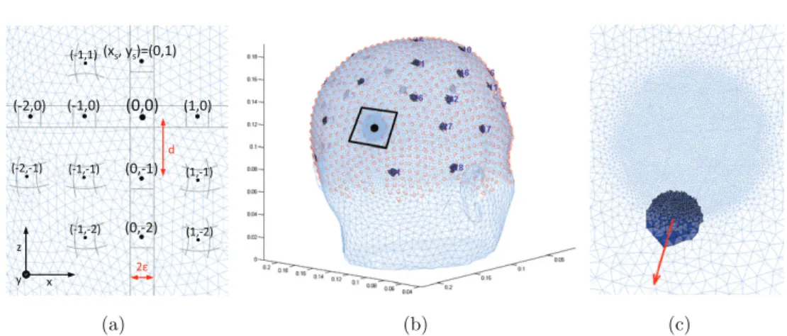
To describe the movement of an electrode along the surface of a mesh, a surface coordinate system is required. We created a surface coordinate system _[x_s×y_s] as follows. Starting from the surface node with the largest y-coordinate (top of the head—(0, 0) in figure 1(a)), we moved along the surface in x and z direction and found surface nodes that are a defined dis-tance d±ε away from the previous point, where ε should be large enough that surface nodes are found. Distance d was chosen such that the surface coordinate points were far enough from each other to describe the surface curvature without significant influence of the mesh discretisation. If no more surface nodes could be found that either fulfilled these requirements or were above a certain y coordinate limit, we stopped. Once the xs and ys axis were found, the four quadrants were filled with points in the same fashion, by averaging the coordinates

of all surface vertices within the area spanned by d±ε (figure 1(a)). To describe directions of movement for each electrode we subsequently found the closest surface coordinate points to that electrode (figures 1(b) and (c)). A mapping back from surface coordinates to mesh nodes was not required. This approach had the advantage that the surface coordinate system could be stored together with the mesh and used for any electrode positions. The Jacobian matrix with respect to electrode radius was computed with a vector field v pointing from the electrode centre to the center of each electrode boundary edge.

For small meshes the electrode boundary Jacobian (EBJ) was calculated in Matlab using a modified version of Eidors (Adler and Lionheart 2006). On the 4 million element mesh used for simulations the EBJ was computed with the Parallel EIT Solver (Peits) (Jehl et al 2015) in order to reduce computing time and memory requirements. The implementation, in our case with linear basis functions, was similar in Matlab and Peits: for each electrode a sparse tem-plate matrix was constructed to store the contributions of drive and measurement fields. For each injection and measurement electrode pair this template matrix could then be multiplied by the electric potential fields of the drive and measurement currents to obtain the EBJ entry for this electrode for this line of the protocol. For the integral along each electrode boundary edge e with end point indices i1 and i2, a [3×3] sub-matrix was added to the template matrix

([ ] [ ]) ( )⎡ ⎣ ⎢ ⎢ ⎤ ⎦ ⎥ ⎥ + = − Γ − − − − n v i i i i i i e z M , , , , , 1/31/6 1/61/3 1/21/2 1/2 1/2 1 , c e

temp 1 2 elec 1 2 elec

elec (10)

where the weights were obtained from Gauss–Lobatto quadrature (a detailed description of the procedure is given in appendix A). Once the template matrices were set up for all electrodes, the drive and measurement fields to multiply them with were the same forward solutions that were required to compute the ‘traditional’ Jacobian matrix and therefore no additional for-ward solutions had to be computed. The computation of one line of the EBJ took on average 0.03 seconds for a 4 m element mesh on ten processors using Peits, whereas one line of Jσ

took around 0.1 s to compute. The additional computation of the EBJ therefore had a minimal effect on the computation time.

Figure 1. Surface coordinate system on 800 k element mesh with one refined electrode: (a) Starting from the top of the head (0, 0), equispaced surface nodes within a tolerance

ε were found in x and z direction. The coordinates of all surface nodes within this tolerance were averaged to define the surface coordinate system. (b) Points of surface coordinate system and (c) 10 mm displacement of electrode number 30 along the xs coordinate (arrow) seen as indicated by the box in (b).

3. Electrode boundary jacobian characteristics

3.1. Simulation parameters

In order to study the characteristics of the voltage changes due to electrode boundary changes, a simulation study was performed on an 800 k element mesh (figure 1(b)). The mesh had refined elements (element size 3 mm instead of 6 mm) in the region where electrodes were located and very fine elements in the vicinity of one electrode (element size 0.4 mm). Current injection was then either simulated to be through a polar electrode pair involving the refined electrode and a coarse electrode on the other side of the head or through adjacent electrodes, again a coarse and the fine one. A representative set of ten different measurement electrode pairs (that were not injecting current) were chosen. The ten measured voltages were sim-ulated for the following permutations: xs coordinate, ys coordinate or electrode diameter change, polar or adjacent injection, fine or coarse electrode. The diameter of 7 mm was altered between ±1.5 mm. Electrode movements were simulated in the range of 0.1–10 mm in both directions and both surface coordinate dimensions. We want to highlight that the mesh was not altered to model the electrode movement. Instead, the assignment of surface facets to the electrodes was used to move the electrodes. This approach was simpler and could account for larger movements of the electrodes.

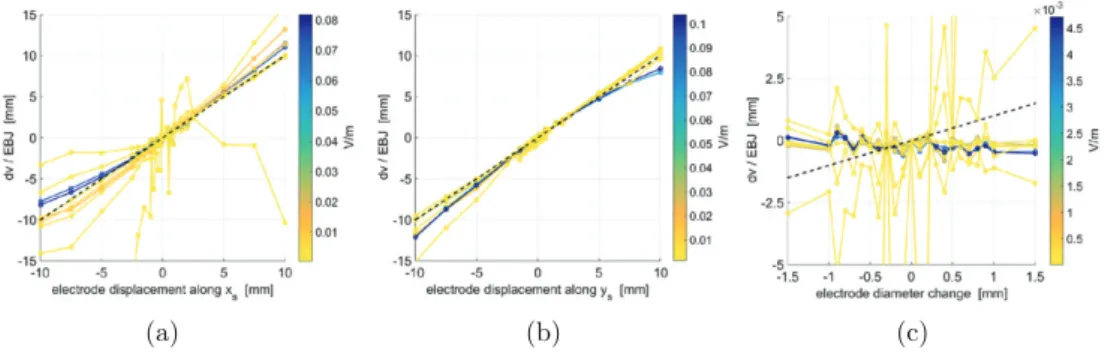
Subsequently, the simulated voltage changes due to the mentioned changes in electrode boundaries were scaled by the changes predicted by the EBJ. This scaling was done in order to be able to show all voltage changes together in one figure, even though they were of different magnitude. The plots of the EBJ accuracy have the simulated electrode change in millimetres on the x-axis and the electrode movement the EBJ would recover given the simulated voltage difference on the y-axis (in millimetres as well). Therefore an optimal prediction of voltage change would result in all 10 curves being perfectly diagonal (black dashed bar in figures 2

and 3). The absolute values of the EBJ with respect to position (both xs and ys) and the EBJ with respect to radius were taken in order to determine which factor was more important. The accuracy of the three different EBJs for the three studied electrodes for adjacent and polar injection was evaluated by linearly interpolating the voltages from simulated electrode bound-ary changes and comparing the slope to the value of the EBJ.

The simulations were performed using a current level of 133 μA and contact impedance of the electrodes (with area E) of zc =1 kΩE on a realistic head mesh (800 k tetrahedral Figure 2. Ratio of actual voltage change over EBJ predicted change for adjacent current injection: (a) for movement of the fine electrode along xs, (b) movement along ys and (c) change in electrode radius (different scaling of x and y axis). The dashed lines represent a perfect prediction of the voltage changes by the EBJ and the colours represent the EBJ amplitude (i.e. large changes are blue, small changes yellow).

elements) with the following layers and corresponding conductivities: scalp (0.44 S m−1_), skull (0.018 S m−1_{), dura mater (0.44 S m}−1_{), cerebrospinal fluid (1.79 S m}−1_{), grey} mat-ter (0.3 S m−1_{) and white matter (0.15 S m}−1_{). The skull was segmented from a CT and the} remaining from an MRI scan of the same subject using Seg3D (CIBC 2014) and meshed with an adapted version of CGAL (CGAL 2015). The ten simulated measurements were the first ten lines of the ‘EEG31’ protocol (Tidswell et al 2001) and for the adjacent injection one of the injecting electrodes was substituted with an adjacent one.

3.2. Voltage dependence on electrode characteristics

3.2.1. Comparison of xs, ys and d prediction of EBJ. The EBJ accurately predicted voltage

changes caused by electrode movement (figure 2). The changes caused by electrode diameter variations were overestimated by the EBJ, and were significantly smaller than the changes caused by electrode movement (colour bar in figure 2).

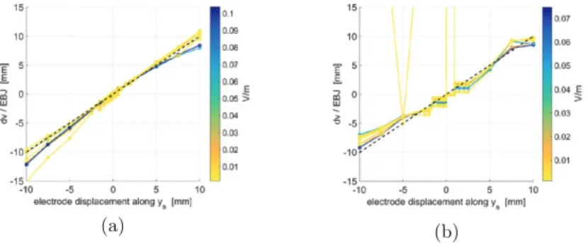
3.2.2. Effect of mesh refinement. The mesh refinement around an electrode did not limit the precision of the EBJ. However, if the electrode positions were corrected on a coarse mesh then the discretisation error was bigger (the big steps in figure 3(b) as opposed to the small steps in figure 3(a)). This is to be expected, since the boundary of the electrode could only change in intervals equal to the element size.

3.2.3. Comparison of polar and adjacent current injection. The voltage changes caused by electrode movement were only minimally different between adjacent and polar current injection (figures 2(b) and 3(a)). This matches expectations, considering that the formula for the computation of the EBJ only depends on electric potential differences at the electrode boundary.

3.3. Precision of electrode boundary jacobian

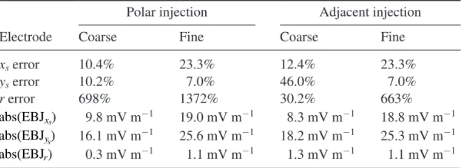
The slopes of simulated voltage changes due to electrode boundary changes were linearly fitted and compared to the EBJ values, to get a measure of the EBJ precision (first three rows of table 1). The voltage changes due to electrode movement were well approximated by the EBJ, with most values having around 10% mismatch. The predicted changes due to elec-trode size changes were on average 690% off. The average absolute values of the EBJ were

Figure 3. Same than figure 2 for movement along ys and polar current injection: (a) on the fine electrode and (b) on the coarse electrode.

compared for the different types of electrode perturbation (movement along xs and ys and change radius r) to illustrate that the changes due to electrode size were significantly smaller than the ones caused by movement (last three rows of table 1).

4. Simulation study

4.1. Time-difference image reconstruction algorithm

In both the simulation study and its experimental validation, we were using spherical pertur-bations in the brain to represent a stroke. We were therefore able to introduce prior informa-tion into our reconstrucinforma-tion by using first order Tikhonov regularisainforma-tion to bias the algorithm towards finding small connected perturbations. All time-difference images were created with a standard least-squares minimisation using generalised singular value decomposition. Many other algorithms have been successfully applied to EIT data (Lionheart et al 2004), and could equally well be used here for simultaneous reconstruction of conductivity changes and elec-trode movements. In the following, we give a brief outline of our time-difference image recon-struction approach.

In EIT, the image reconstruction problem can be described by the minimisation of the cost functional p x , 1 F x v F x v x D Dx 2 1 2 x 2 1 ( (σ )) ( ( ) ) ( ( ) ) λ Φ ₍₁₁₎= − − + Γ−

with x the change in conductivity and electrode positions we wish to reconstruct, v the voltage difference between the two measurements, F x_{( )} a non-linear function relating conductivity and electrode position changes to voltage changes, Γx the expected variance of the

recon-structed variables (conductivities Γσ and positions Γp)

⎡ ⎣⎢ ⎤ ⎦⎥ ⎡ ⎣⎢ ⎤ ⎦⎥ I I 0 0 std 0 0 std x p p x x 2 Γ ₍₁₂₎= Γσ _Γ = σ⋅ _⋅ =Σ Σ

and the first order Tikhonov regularisation term for the conductivities combined with zero order Tikhonov for the electrode positions

⎡ ⎣⎢ ⎤⎦⎥ D D L L I 0 0 . = (13) Using the substitution Dx=Σ−x1D and linearising F x( ) around the model values of x then

gives

Table 1. Error and amplitudes of the EBJ for different types electrode boundary changes. All values are the average of 10 different measurements.

Polar injection Adjacent injection

Electrode Coarse Fine Coarse Fine

xs error 10.4% 23.3% 12.4% 23.3% ys error 10.2% 7.0% 46.0% 7.0% r error 698% 1372% 30.2% 663% ( ) abs EBJxs 9.8 mV m−1 19.0 mV m−1 8.3 mV m−1 18.8 mV m−1 ( ) abs EBJys 16.1 mV m−1 25.6 mV m−1 18.2 mV m−1 25.3 mV m−1 ( ) abs EBJr 0.3 mV m−1 1.1 mV m−1 1.3 mV m−1 1.1 mV m−1

x 1 Jx v Jx v x D D x 2 1 2 x x 2 ( ) ( ) ( ) λ Φ ₍₁₄₎= − − +

and the minimum can be found by setting the derivative to zero

x 0 J Jx v 2D D x_x x

( ) ( ) λ

Φ ₍₁₅₎′ = = − +

Using the generalised singular value decomposition (gSVD) of the Jacobian J and scaled regularisation matrix Dx this equation can be solved for x

x=(J J +λ2D D_x x)−1J v =X(Λ Λ +λ2M M )−1ΛU v,

(16) where J=U XΛ _{and D VMX}

x= . Since both Λ and M are diagonal matrices with a limited

number of generalised singular values (Hansen 1994), they can easily be inverted.

To reduce the computational cost of calculating the gSVD and to prevent the ‘inverse crime’

(Lionheart et al 2004) we used a much smaller hexahedral mesh (2526 elements of 1× ×1 1 cm) for the image reconstructions (figure 4(a)). The Jacobian matrix Jσ which was computed

on the fine mesh was summed into geometrically regular cubes Jhex and the Laplacian matrix L for the first order Tikhonov regularisation was computed on this hexahedral mesh. In order to simultaneously reconstruct conductivity changes and electrode movements, the ‘traditional’

Jacobian matrix Jhex had to be combined with the EBJ as J=[Jhex EBJ]. Equivalently, if

only the conductivity changes or only the electrode movements were reconstructed, only the relevant Jacobian matrix and the corresponding part of D was used.

The expected variance of the conductivity was set to varσ=0.1 S m−1 and for the electrode positions to varp=1 mm. For all reconstructed images and electrode positions, the regularisa-tion factor _{λ =}2 2.1 10_⋅ −7 _{was kept constant. The value was chosen based on the shape of the}

L-curve (Hansen 1994), however the L-curve was not pronounced enough to choose λ in an automated way. The solution norm ∥ ∥x 2 for our choice of λ was generally around 0.1 and the

residual norm ∥Jx−v∥2 around 1.0 10⋅ −4. The colour bar of all images was scaled according

to the largest reconstructed change in the whole mesh. Therefore images of slices sometimes do not contain the maximum value of the colour bar.

4.2. Image quantification

In order to evaluate the image quality objectively, three quantification methods were applied. The volume P corresponding to the reconstructed perturbation was identified as the largest connected cluster of voxels with 50% of the maximum of the image (Malone et al 2014). The Figure 4. Slices through the coarse hexahedral mesh used for reconstruction: (a) baseline conductivities (b) conductivity change when a plastic perturbation of 0.0001 S m−1 _{was inserted in the back of the head.}

region of interest (ROI) was defined as the largest connected cluster of voxels with 50% of the maximum of the simulated conductivity change.

• Localisation error: ratio between the displacement (x y zP, ,P P) of the centre of mass of

the reconstructed perturbation P from the actual perturbation location, and the average dimension of the mesh (d d dx, ,y z)

x y z d d d , , mean , , . P P P x y z ∥( )∥ ( ) (17)

• ROI change: difference of the average value of the reconstructed image (dσr) in the ROI

and the average value of the actual perturbation (dσa), divided by the average value of the

perturbation

f mean d mean d

mean d ,

r a

a

tikh ROI ROI

ROI ( ) ( ) ( ) σ σ σ ⋅ − (18) where the Tikhonov smoothing correction factor f_tikh corrects for the effect that the

reconstructed perturbation is larger in volume and smaller in amplitude by scaling the reconstructed conductivity change within the ROI (f_tikh =10 was used throughout).

• ROI noise: noise-to-signal ratio of the reconstructed image (dσr), computed as the ratio

between the standard deviation (std) outside the ROI and the average value in the ROI

std d mean d . r r \ROI ROI ( ) ( ) σ σ Ω (19) 4.3. Simulation parameters

Jσ and EBJ for the image reconstructions in the simulation study and tank experiments were

computed on the same 4 m element human head mesh with a homogeneous saline background of 0.4 S m−1 _{conductivity and a realistic human skull with variable conductivities between} 0.0094 S m−1 _{and 0.025 S m}−1 _{(Tang et al 2008). The current level was 250 μA, contact} impedances of all electrodes were set to zc = 220 Ω ⋅E and the diameter of the 32 electrodes was 10 mm. The plastic perturbation had a radius of 1.5 cm and a conductivity of 0.0001 S m−1 (figure 4(b)). The injecting pairs of electrodes were chosen to maximise the distance between electrodes by finding the maximum spanning tree, weighted by the inter-electrode distances. Measurements were made for each injection on all adjacent electrode pairs not involved in delivering the current, giving a total of 869 measured voltages from 31 independent current injections. All voltages, the conductivity Jacobian matrix and the EBJ were computed with Peits (Jehl et al 2015).

The level of noise added to simulated differential voltages was chosen to match the experi-ments and consisted of ς =p 0.006% proportional noise and ς =a 1 μV additive noise, such that

vwith noise  =vno noise  (1+rand( ))ςp +rand( )ςa ,

(20) where rand_{( )}ς indicates random numbers drawn from a Gaussian distribution with zero mean and standard deviation ς.

4.4. Electrode position recovery

To reconstruct conductivities and electrode positions simultaneously, the algorithm outlined in section 4.1 is used. Analogously, if only electrode positions are reconstructed, then the

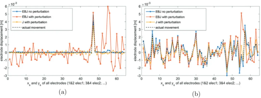
full Jacobian is replaced by only the EBJ. The performance of the EBJ for electrode posi-tion recovery was validated with three different recovery modalities: (1) only the EBJ was used to recover electrode positions when the electrodes moved and the conductivities did not change; (2) only EBJ was used when electrode positions and conductivity (plastic ball in back of the head) changed; (3) the full Jacobian matrix was used to reconstruct conductivities and electrode movement at the same time when both electrode positions and conductivity have changed. All these differently recovered electrode positions were plotted together with the actual electrode movement for two cases, one where only one electrode on the back of the head moved by 5 mm (figure 5(a)) and the other one where all electrodes were moved along both xs and ys by random values with standard deviation 1 mm (figure 5(b)).

The 2-norm of the difference of recovered movement versus actual movement shows that the simultaneous reconstruction of a conductivity perturbation and electrode movements (last row in table 2) was close to that of the sole recovery of the electrode positions when no pertur-bation was introduced (first row in table 2). Contrastingly, if the conductivity changed simul-taneously with the electrode positions, the recovery of only the electrode positions resulted in a significant over-correction (second row in table 2), especially close to where the perturbation was introduced (numbers 41–64 in figures 5(a) and (b) corresponding to xs and ys coordinates of electrodes 21–32 towards the back of the head).

4.5. Images

The best possible images (i.e. in the presence of no electrode movement) that were achiev-able with time-difference reconstructions without electrode correction (figure 6(a)) and with electrode correction (figure 6(d)) were qualitatively similar. The simultaneous reconstruction of conductivity and electrode positions slightly reduced the contrast and the precision of the imaged perturbation.

If one electrode in the top back of the head was moved by 5 mm, the simple time-differ-ence reconstruction resulted in an unsurprisingly noisy image (figure 6(b)) with large artefacts

Figure 5. Recovered electrode movement for three different cases: only EBJ was used and only the electrode positions changed, only EBJ was used and additionally to the electrode movement a perturbation was inserted at the back of the head, and the complete Jacobian J was used when both electrodes and conductivity changed. In (a) an electrode on the back of the head was moved along xs by 5 mm and in (b) all electrodes were moved along xs and ys by a random value. On the x axis of these two plots the entries 1 and 2 correspond to the xs and ys coordinate of electrode 1, then the next two entries correspond to electrode 2 and so on.

around the moved electrode. Simultaneous reconstruction of the electrode positions (figure

6(e)) restored the quality of the image almost to the ideal case (figure 6(a)).

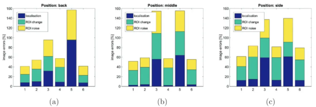
As with a large movement of one single electrode, smaller movements of all electrodes had a detrimental effect on the image quality for simple time-difference imaging (figure 6(c)). The image reconstructed with the full Jacobian was again largely unaffected by this large degree of electrode movement (figure 6(f)). All these findings were summarised for three different posi-tions of the perturbation by assessing the image quality according to the previously defined error metrics (figures 7(a)–(c)). The larger localisation error (and inherently larger ROI errors) for a perturbation on the side can be explained by the reduced sensitivity of the current proto-col used for these simulations.

5. Experimental validation

5.1. Experimental setup

Two saline tanks were printed using the 3D printer Makerbot Replicator 2 from Makerbot Ind. The model for the tank was created from the same MRI segmentation used for the mesh creation, whereas the skull was segmented from a corresponding CT scan. The skull model Table 2. 2-norm of the difference of recovered electrode movement and actual electrode movement.

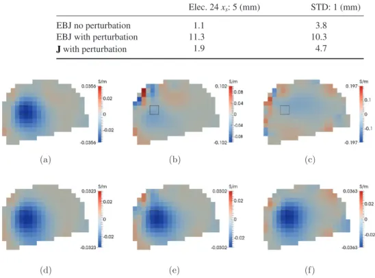
Elec. 24 xs: 5 (mm) STD: 1 (mm)

EBJ no perturbation 1.1 3.8

EBJ with perturbation 11.3 10.3

J with perturbation 1.9 4.7

Figure 6. Slice through the reconstructed image of a simulated perturbation (black outline) in the back of the head without (first row) and with (second row) electrode movement correction: (a), (d) when electrodes have not moved, (b), (e) when electrode 24 (top back of the head) moved along xs by 5 mm and (c), (f ) when all electrodes moved along xs and ys by normally distributed distances with standard deviation 1 mm.

(a) (b) (c)

was further edited by introducing small holes, such that the conductivity matched that of a real skull (Avery 2015). One tank was printed with a modified EEG 10–20 electrode placement (Tidswell et al 2001, Avery 2015) and the other tank had perturbed electrode positions with random displacements along xs and ys with standard deviation of 1 mm, matching the electrode movement simulated in section 4.

For the recordings, the tanks were filled with 0.4 S m−1 _{saline. The electrode contact} imped-ances were measured to be 220 Ω ⋅E. Current was injected at 1.76 kHz with 250 μA ampli-tude, to approximately match the allowed current level in human measurements (Dybdahl

2009). A slightly modified 32-channel version of the KHU Mark 2.5 system (Wi et al 2014) was used for the recordings and each measurement was repeated 20 times over the course of approximately one minute. Plastic perturbations with 3 cm diameter were placed in approxi-mately the same locations used in the simulations.

5.2. Images

With baseline and perturbation measurements in the same saline tank, both using Jhex and using J resulted in a reconstruction of the perturbation with only minimally worse quality than for simulated noisy voltages (figures 8(b) and (c) and the first two bars in the quality measures in figure 9). However, when reconstructing a perturbation measured in the tank with the moved electrodes, then large artefacts in the outer layers of the head near the skull were observed (figures 8(d) and (e)). These artefacts strongly influenced the localisation errors (figure 9), where an artefact was interpreted as the reconstructed perturbation. The drop in image quality was most likely caused by small differences in skull placement in the two different saline tanks.

Simultaneous reconstruction of conductivities and electrode movements improved the image visibly (figure 8(e)), but did not remove all artefacts. Since electrode movement cannot completely account for all voltage changes, artefacts caused by other effects (such as skull position in the two tanks) remain in the conductivity image. Parts of the voltage differ-ences caused by these geometrical differdiffer-ences were, however, pulled into the electrode move-ment recovery. Therefore, the precision of the recovered electrode movemove-ment between the two

Figure 7. Image quantification results for simulations of: (a) a perturbation in the back, (b) a perturbation in the middle and (c) a perturbation on the side. 1 and 2 are the error metrics for reconstructions without and with electrode correction when the electrodes have not moved. 3 and 4 are the metrics for reconstructions without and with electrode correction when electrode 24 in the top back of the head was moved along xs by 5 mm. And 5 and 6 are the same metrics in the case of random movements of all electrodes with a standard deviation of 1 mm.

3D printed tanks was lower than in simulations (error 2-norm 8.0 mm instead of 4.7 mm in simulations).

6. Absolute reconstructions

6.1. Absolute reconstruction algorithm

In contrast to time-difference imaging, absolute reconstructions do not require a base-line measurement. In many realistic applications, absolute imaging fails—among other

Figure 8. (a) The KHU Mark 2.5 system and the 3D printed head shaped tank with realistic 3D printed skull. (b)–(e) Slices through the reconstructed image of a plastic ball in the 3D printed head tank with realistic skull without (left column) and with (right column) electrode movement correction: (b), (c) when baseline and perturbation measurements were done in the tank with the correct electrode positions and (d), (e) when the baseline was measured in the tank with the correct electrode positions and the perturbation measurement was done in the tank with the electrodes shifted by random values with standard deviation 1 mm in both surface directions.

(a)

(b) (c)

(d) (e)

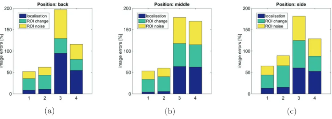
Figure 9. Image quantification results for experimental images with: (a) a plastic perturbation in the back, (b) a plastic perturbation in the middle and (c) a plastic perturbation on the side. 1 and 2 are the error metrics for reconstructions without and with electrode correction when the electrodes have not moved. And 3 and 4 are the same metrics in the case of random movements of all electrodes with a standard deviation of 1 mm.

for the search direction dk. The reconstructed change in conductivity and electrode positions

was then updated in each iteration α

= +

+

xk 1 xk k kd ,

(22) where αk is the step size and was optimised using the Brent line search method (Brent 1973)

with a gold-section bracketing loop to find the Brent abscissae. Analogous to the time-dif-ference approach, the reconstructions were weighted by the expected variance. In iterative reconstructions it is important to ensure the positivity of the elements’ conductivity in the Gauss–Newton step, which was done here by using the substitution

⎡ ⎣ ⎢ ⎢ y p log std std_p , 1 1 ( σ) = σ − − (23)

where x=[σ,p]_{. Applying this substitution to (21) moved the scaling by the expected}

stan-dard deviation of the variables from the regularisation term to the Jacobian matrix, making the Jacobian dimensionless. According to the chain rule, the logarithmic part of the substitution results in a multiplication of the Jacobian entries corresponding to conductivities by eσ_{. After}

+

y_{k 1} was found using Gauss–Newton, the electrode positions and conductivities were updated according to the corresponding xk+1.

The regularisation parameter for all absolute reconstructions was set to _{λ =}2 10−11 _{and the}

stopping criterion was set to <10−7 _{change between iterations with a maximum of 6} itera-tions. As a trade-off between computational efficiency and precision of the forward solutions, a tetrahedral mesh with 1 million elements was used for the absolute reconstructions.

6.2. Images

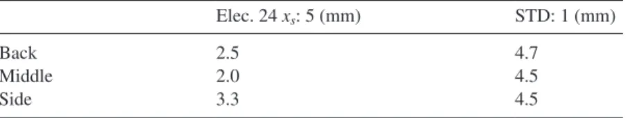
All absolute reconstructions from simulated data had a large positive artefact in the front of the head, where the sensitivity is high. When the full Jacobian matrix was used, the algorithm unsuccessfully tried to reduce this artefact by moving the electrodes in the front of the head (left side of figure 10(c)). When evaluating the recovery of electrode movements, we therefore subtracted this ‘baseline’ movement from the reconstructed movement of the electrodes when they have actually moved. Doing this, we found a good performance of the iterative electrode movement correction (table 3, as compared to the last row in table 2). The large artefact results in a poor image quantification score for all reconstructed images, with or without inclusion of the EBJ. Subsequently, we illustrate the difference the electrode correction makes by show-ing one reconstruction without and with EBJ, both thresholded to one third of the maximum reconstructed change (figure 10).

We were not able to reconstruct meaningful absolute images from the experimental data. Even on the tank with no electrode movement the reconstructions did not show the perturbation.

7. Discussion

7.1. Electrode boundary jacobian characteristics

We observed that the measured voltages changed linearly with electrode movement over 1 cm and were very accurately predicted by the EBJ (the linearity was already observed multiple times, as reviewed in Kolehmainen et al (1997)). There were outliers where some voltages did behave highly non-linearly (figure 2(a)), but as seen from the colour coding these outliers were of small amplitude. Therefore they were not expected to adversely influence the recon-struction of electrode movements. Changes in electrode diameter had a less predictable influ-ence on the measured voltages (figure 2(c)). Firstly, the EBJ predicted changes were between one and two orders of magnitude smaller than for electrode movements and, secondly, the observed voltage changes were even smaller than the EBJ predictions. Changes in electrode shape can be viewed as a combination of a change in diameter and the discretisation errors seen in the electrode movement on the coarse electrode (figure 3(b)). Therefore these changes can be expected to be small, even though we did not analyse this specifically. We concluded that changes in electrode size and shape could be ignored in the presence of electrode move-ment, and that they were not very well approximated by the EBJ. The focus of the simulation study and the experiments was therefore laid on the correction of electrode movements, which had the strongest impact on the image quality.

The mesh refinement around the electrode had no influence on the precision of the EBJ (figure 3), which indicated that meshes did not have to be altered for the use of electrode movement correction. Electrodes could be moved by simply assigning different surface facets to the electrode, without introducing errors larger than the discretisation errors caused by the element size. This facilitated the electrode movement correction significantly, since the mesh Figure 10. Reconstructed absolute images of a simulated perturbation in the back of the head when all electrodes were moved along xs and ys by normally distributed random distances with standard deviation 1 mm: (a) reconstruction without using the EBJ and (b) reconstruction with EBJ. Both reconstructions were thresholded at ±33% of the maximum change. (c) Comparison of the recovered electrode movement when using the original electrode positions, and when electrode 24 was moved by 5 mm along xs (dashed black line).

(a) (b) (c)

Table 3. 2-norm of the difference of reconstructed electrode movement and actual electrode movement for different perturbation locations.

Elec. 24 xs: 5 (mm) STD: 1 (mm)

Back 2.5 4.7

Middle 2.0 4.5

thereby reduce the image noise notably. In the presence of image artefacts which were not caused by electrode movement, using the EBJ resulted in a less precise reconstruction of the electrode positions. This was because the reconstruction algorithm reduced the cost functional by moving parts of the image artefact into the electrode positions. However, since 64 param-eters constituting the positions of the 32 electrodes could not account for these artefacts, they were still visible in the resulting conductivity image.

7.3. Experimental validation

Time-difference reconstructions in the printed head tank with the correct electrode positions gave good results. Using the baseline measurement with the correct tank and the perturbation measurement on the tank with changed electrode positions resulted in noisier images than in the corresponding simulations. The additional noise was most likely caused by small geo-metrical differences in the skull positioning in the two different tanks, slightly different saline levels between the measurements and ambient and system temperature differences. While such errors were not present in conventional time-difference measurements, they manifested themselves when two different tanks were used with a half an hour break in between setting up each tank. Still, the simultaneous reconstruction of conductivity and electrode movement significantly improved the reconstructions and allowed for the detection of the perturbation. 7.4. Absolute reconstructions

The iterative absolute recovery of electrode positions was accurate and strongly reduced the electrode movement related artefacts. Still, the absolute conductivity reconstructions with or without electrode correction showed a systematic artefact in the front of the head. This was in a region of strong sensitivity and might have been exacerbated by the comparative imprecision of the skull in the one million element mesh used for the absolute reconstructions. Moving to a finer, more precise mesh would result in very long computation times even for a single image reconstruction.

We were not able to get meaningful absolute reconstructions from the experimental data, suggesting that the simulations and experiments were still too different even though the geom-etry of the tank and inserted skull were printed with a precision of 0.2 mm. However, the plac-ing of the skull in the tank was less precise than this. More advanced absolute reconstruction algorithms might be able to retrieve more information from our experimental data by includ-ing geometrical uncertainties around the skull into the imaginclud-ing method.

7.5. Conclusions

We have applied the Fréchet derivative of the EIT forward problem with respect to electrode boundary changes to a realistic 3D model of the human head, using a fast implementation. This allowed us to reconstruct the conductivities and electrode positions simultaneously, and

therefore make reconstructions more stable in the presence of electrode movement. For this realistic EIT setting we have found that:

(i) The electrode position has a much stronger effect on the boundary voltages than the electrode diameter and shape. The voltages changed linearly for electrode movements up to 1 cm and were accurately predicted by the EBJ.

(ii) The simultaneous reconstruction of conductivity and electrode positions worked very well. Image artefacts caused by electrode movements were reliably removed and the electrode positions were accurately corrected. The positive results of the simulation study were confirmed in experiments on a 3D-printed saline tank containing a realistic 3D-printed skull.

(iii) While the correction of electrode movements was accurate in iterative absolute imaging as well, the absolute conductivity reconstructions from simulated data had a large artefact in the front of the head. No meaningful absolute images could be reconstructed on the 3D-printed saline tank.

We conclude, that the proposed application of the EBJ works well in time-difference recon-structions and can be used for long term monitoring of physiological changes. For stroke type differentiation, time-difference measurements are not possible. Therefore, existing multi-frequency reconstruction algorithms need to be adapted to correct for imprecisely modelled electrode positions using the EBJ.

Appendix A. Template EBJ construction

The integral along the electrode boundary (9) can be decomposed into a sum of the integrals over each element edge, from node i1 to node i2. To compute this integral, the drive and mea-surement potential field values at the two nodes and the corresponding electrode elec have to be known. For our implementation, we were using Gauss–Lobatto quadrature with three points to approximate the integral along one edge. The Gauss–Lobatto weights on a unit inter-val are given as w1 = 1/6, w2 = 4/6 and w3 = 1/6 and therefore the integral along one edge e can be approximated as

∫

elec elec elec elec

elec elec elec elec elec elec m m 1 1 2 2 ( )( ˜ ˜) ( ˜ ˜) ( )( ˜ ˜ ) ( )( ˜ ˜ ) ( )( ˜ ˜ ) (A.1)

Since we were using linear shape functions, the voltage at the midpoint im was given by

uim= 1₂(ui1+ui2). Calculating out and writing as a matrix vector multiplication, (A.1) is

equivalent to ⎡ ⎣ ⎢ ⎢ ⎤ ⎦ ⎥ ⎥ U u U u d m f , , , 1/31/6 1/61/3 1/21/2 1/2 1/2 1 , e e elec elec ( ˜ ˜)= −− − −

⎣ ⎢ ⎢ _⎦⎥⎥ d m n v d m d m z EBJelec, , 1/6 1/3 1/2 M 1/2 1/2 1 elec . e c elec e e e temp ( )=

∑

Consequently, we could create one sparse [#nodes+#elec×#nodes+#elec] template matrix

Mtemp for each electrode by summing the contributions of all electrode boundary edges into the

corresponding indices i1, i2 and ielec. These #elec template matrices could then be multiplied

with all used combinations of d=[u U, ] _{and m=[ ˜ ˜ ]u U, to obtain the [#prt_lines×#elec]}

electrode boundary Jacobian with respect to vector field v.

References

Adler  A and Lionheart  W 2006 Uses and abuses of EIDORS: an extensible software base for EIT Physiol. Meas. 27 25_–42

Avery J 2015 Improving electrical impedance tomography of brain function with a novel servo-controlled electrode helmet PhD Thesis University College London

Boyle A, Adler A and Lionheart W 2012 Shape deformation in two-dimensional electrical impedance tomography IEEE Trans. Med. Imaging 31 2185_–93

Brent R 1973 Algorithms for Minimization Without Derivatives (New York: Dover) CIBC 2015 Seg3d: volumetric image segmentation and visualization (www.seg3d.org) CGAL 2015 Computational Geometry Algorithms Library (www.cgal.org)

Dard_é J, Hakula H, Hyv_önen N and Staboulis S 2012 Fine-tuning electrode information in electrical impedance tomography Inverse Problems Imaging 6 399_–421

Dard_é  J, Hyv_önen  N, Sepp_änen  A and Staboulis  S 2013 Simultaneous recovery of admittivity and body shape in electrical impedance tomography: an experimental evaluation Inverse Problems

29 85004_–19

Dybdahl K 2009 Patient protection at risk in IEC 60601-1 3rd edition Med. Device Technol. 20 26–8 G_ómez-Laberge  C and Adler  A 2008 Direct EIT jacobian calculations for conductivity change and

electrode movement Physiol. Meas. 29 89_–99

Hansen P 1994 Regularization tools: a matlab package for analysis and solution of discrete Ill-posed problems Numer. Algorithms 6 1_–35

Heikkinen  L, Vilhunen  T, West  R and Vauhkonen  M 2002 Simultaneous reconstruction of electrode contact impedances and internal electrical properties: II. Laboratory experiments Meas. Sci. Technol. 13 1855_–61

Jehl M, Dedner A, Betcke T, Aristovich K, Kl_öfkorn R and Holder D 2015 A fast parallel solver for the forward problem in electrical impedance tomography IEEE Trans. Biomed. Eng. 62 126_–37

Jun S, Kuen J, Lee J, Woo E, Holder D and Seo J 2009 Frequency-difference EIT fdEIT using weighted difference and equivalent homogeneous admittivity: validation by simulation and tank experiment Physiol. Meas. 30 1087_–99

Kolehmainen V, Vauhkonen M, Karjalainen P and Kaipio J 1997 Assessment of errors in static electrical impedance tomography with adjacent and trigonometric current patterns Physiol. Meas. 18 289_–303

Lionheart W, Polydorides N and Borsic A 2004 Electrical Impedance Tomography: Methods, History and Applications ed D S Holder (London: Taylor and Francis) 3_–64 (chapter 1)

Malone E, Jehl M, Arridge S, Betcke T and Holder D 2014 Stroke type differentiation using spectrally constrained multifrequency EIT: evaluation of feasibility in a realistic head model Physiol. Meas.

35 1051_–66

Malone  E, Sato Dos Santos  G, Holder  D and Arridge  S 2013 Multifrequency electrical impedance tomography using spectral constraints IEEE Trans. Med. Imaging 33 340_–50

Nissinen A, Heikkinen L and Kaipio J 2008 The bayesian approximation error approach for electrical impedance tomography_—experimental results Meas. Sci. Technol. 19 015501

Polydorides  N and Lionheart  W 2002 A Matlab toolkit for three-dimensional electrical impedance tomography: a contribution to the electrical impedance and diffuse optical reconstruction software project Meas. Sci. Technol. 13 1871_–83

Soleimani  M, G_ómez-Laberge  C and Adler  A 2006 Imaging of conductivity changes and electrode movement in EIT Physiol. Meas. 27 S103_–13

Somersalo E, Cheney M and Isaacson D 1992 Existence and uniqueness for electrode models for electric current computed tomography SIAM J. Appl. Math. 52 1023_–40

Tang C, You F, Cheng G, Gao D, Fu F, Yang G and Dong X 2008 Correlation between structure and resistivity variations of the live human skull IEEE Trans. Biomed. Eng. 55 2286_–92

Tidswell  T, Gibson  A, Bayford  R and Holder  D 2001 Three-dimensional electrical impedance tomography of human brain activity NeuroImage 13 283_–94

Wi H, Sohal H, McEwan A, Woo E and Oh T 2014 Multi-frequency electrical impedance tomography system with automatic self-calibration for long-term monitoring IEEE Trans. Biomed. Circuits Syst. 8 119_–28

Xu C, Wang L, Shi X, You F, Fu F, Liu R, Dai M, Zhao Z, Gao G and Dong X 2010 Real-time imaging and detection of intracranial haemorrhage by electrical impedance tomography in a piglet model J. Int. Med. Res. 38 1596_–604