CYBERGIS-ENABLED REMOTE SENSING DATA ANALYTICS FOR DEEP LEARNING OF LANDSCAPE PATTERNS AND DYNAMICS
BY ZEWEI XU
DISSERTATION
Submitted in partial fulfillment of the requirements for the degree of Doctor of Philosophy in Geography
in the Graduate College of the
University of Illinois at Urbana-Champaign, 2020
Urbana, Illinois
Doctoral Committee:
Professor Shaowen Wang, Chair Assistant Professor Kaiyu Guan
Assistant Professor Zhe Jiang, University of Alabama Professor Bruce Rhoads
ABSTRACT
Mapping landscape patterns and dynamics is essential to various scientific domains and many practical applications. The availability of large-scale and high-resolution light detection and ranging (LiDAR) remote sensing data provides tremendous opportunities to unveil complex landscape patterns and better understand landscape dynamics from a 3D perspective. LiDAR data have been applied to diverse remote sensing applications where large-scale landscape mapping is among the most important topics. While researchers have used LiDAR for understanding landscape patterns and dynamics in many fields, to fully reap the benefits and potential of LiDAR is increasingly dependent on advanced cyberGIS and deep learning
approaches. In this context, the central goal of this dissertation is to develop a suite of innovative cyberGIS-enabled deep-learning frameworks for combining LiDAR and optical remote sensing data to analyze landscape patterns and dynamics with four interrelated studies. The first study demonstrates a high-accuracy land-cover mapping method by integrating 3D information from LiDAR with multi-temporal remote sensing data using a 3D deep-learning model. The second study combines a point-based classification algorithm and an object-oriented change detection strategy for urban building change detection using deep learning. The third study develops a deep learning model for accurate hydrological streamline detection using LiDAR, which has paved a new way of harnessing LiDAR data to map landscape patterns and dynamics at
unprecedented computational and spatiotemporal scales. The fourth study resolves computational challenges in handling remote sensing big data and deep learning of landscape feature extraction and classification through a cutting-edge cyberGIS approach.
ACKNOWLEDGMENTS
This dissertation would not have been possible without the extraordinary guidance, help, and encouragement from my mentors, friends, and family. They make my PhD study at UIUC an exciting and memorable journey.
I would like to start by expressing my deepest gratitude to my advisor, Dr. Shaowen Wang. The past several years have not been an easy ride and I have learned numerous things from him, academically and spiritually. Throughout my time with him, he selflessly shares his wisdom of researching with me and constantly supports me when I hit nadirs in life. I still
remember the numerous times when I struggled with research roadblocks and life unfortunates. It was he who taught me the importance of perseverance in doing research and encouraged me to get through my dark times. I would also like to thank Dr. Kaiyu Guan, Dr. Zhe Jiang for their patient and rigorous guidance. Their research enthusiasm and meticulousness encourage me throughout my journey with them. My appreciation also goes to Dr. Bruce Rhoads and Dr. E. Lynn Usery, who inspired me a lot during my PhD study and defense, and provided practical and valuable suggestions for my dissertation work.
Moreover, I would like to thank my best friends and colleagues in the Department of Geography and Geographic Information Science and Cyberinfrastructure and Geospatial Information Laboratory for their care, support, and companionship during the past six years. Many of these people have become my lifetime friends. Meanwhile, I want to give special thanks to Matthew Cohn, Susan Etter, and Miranda Czerwonka for their years of help and support.
Finally, I would like to thank my family for their unconditional love and support for my PhD study journey. I am extremely grateful to my father, Yuezhong Xu, who taught me the importance of self-discipline and positive thinking. And also my Mom, Xifeng Hu, who makes
me always believe in myself and also be kind and compassionate to others. There are always not enough words to express my appreciation for their sacrifices and love. Lastly, I am thankful for the patience of my future wife and unborn children, I will have more time to find and be with you from now on.
This dissertation research is based in part upon work supported by the U.S. National Science Foundation under grants: ACI-1443080, ICER-1833225, and OAC-1743184; and U.S. Geological Survey CESU Grant #G14AC00244. Any opinions, findings, and conclusions or recommendations expressed in this material are those of the authors and do not necessarily reflect the views of the National Science Foundation and the U.S. Geological Survey.
TABLE OF CONTENTS
CHAPTER 1: INTRODUCTION AND BACKGROUND ... 1
1.1 Motivation and vision... 1
1.1.1 Landscape patterns and dynamics ... 2
1.1.2 Artificial Intelligence for geospatial research ... 2
1.1.3 Remote sensing data analytics and cyberGIS ... 3
1.2 Research problems and questions ... 4
1.3 Remote sensing and deep learning methods ... 7
1.3.1 Optical remote sensing ... 8
1.3.2 LiDAR remote sensing ... 9
1.3.3 Deep learning ... 11
1.4 Structure of the dissertation ... 14
1.5 Synthesis and contribution... 17
1.6 Publications ... 18
CHAPTER 2: A 3D CONVOLUTIONAL NEURAL NETWORK METHOD FOR LAND COVER CLASSIFICATION USING LIDAR AND MULTI-TEMPORAL LANDSAT IMAGERY... 20
2.1 Introduction and background... 21
2.2 Study area and dataset... 24
2.2.1 Study area... 24 2.2.2 Dataset ... 25 2.3 Methods... 26 2.3.1 Method overview... 26 2.3.2 Sampling design ... 27 2.3.3 Data preprocessing... 28 2.3.4 Benchmark method ... 30
2.3.5 3D CNN-based multi-stage classification ... 32
2.4 Results ... 39
2.4.1 Overall performance ... 39
2.4.2 Classification accuracy on different classes ... 41
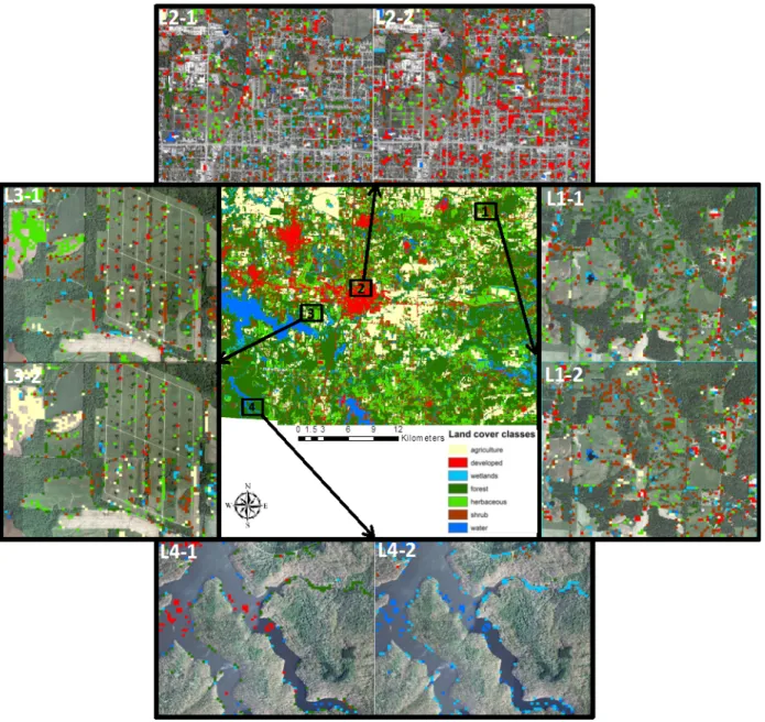
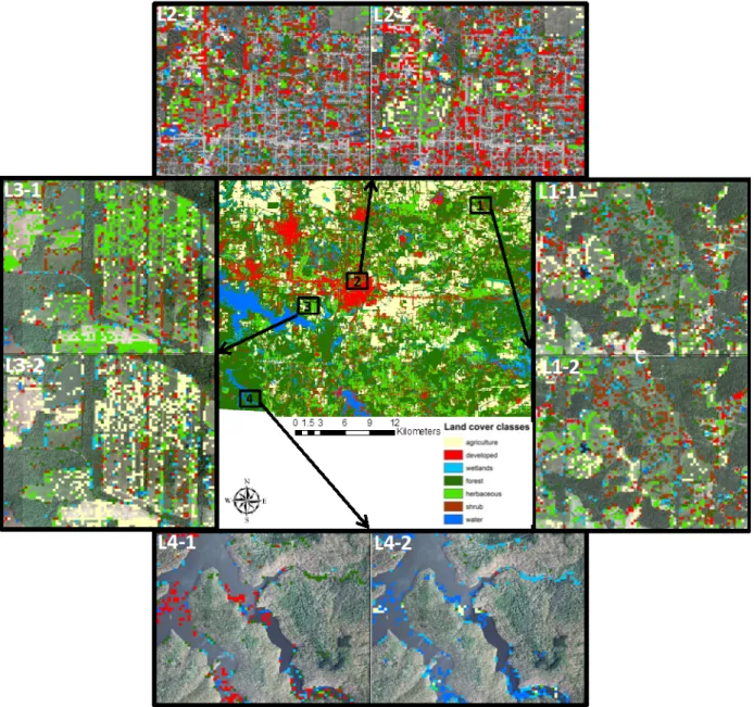
2.4.3 Characteristics of spatial distribution of classified land cover types ... 44
2.5 Conclusions and discussion ... 46
2.6 Supplementary ... 49
CHAPTER 3: URBAN BUILDING EXTRACTION AND CHANGE DETECTION USING MULTITEMPORAL LIDAR DATA BASED ON A DEEP LEARNING AND RULE-BASED METHOD ... 52
3.1 Introduction ... 53
3.2 Background ... 57
3.2.1 Study area... 57
3.2.2 Multi-temporal LiDAR dataset... 58
3.2.3 Reference dataset ... 59
3.3.1 Data preprocessing... 60
3.3.2 Point-based classification ... 62
3.3.3 Euclidean clustering and 3D building model construction ... 64
3.3.4 Building change detection and 3D change volume estimation... 65
3.3.5 Validation ... 67
3.4 Results ... 67
3.4.1 Accuracy evaluation of building classification ... 68
3.4.2 Accuracy assessment of building volume estimation ... 72
3.4.3 Accuracy evaluation of building change detection ... 72
3.4.4 Visualization of different change types and wrong detections ... 76
3.5 Discussions... 78
3.6 Conclusion ... 81
CHAPTER 4: HYDROLOGICAL STREAMLINE DETECTION USING A U-NET MODEL ... 83
4.1 Introduction ... 84
4.2 Study area and dataset... 88
4.3 Methods... 94
4.3.1 Benchmark methods... 94
4.3.2 The U-net model ... 95
4.4 Result ... 101
4.5 Conclusion and Discussion ... 105
CHAPTER 5: AN INTEGRATED CYBERGIS AND DEEP-LEARNING FRAMEWORK FOR SCALABLE LAND COVER MAPPING USING LIDAR AND LANDSAT REMOTE SENSING 109 5.1 Introduction ... 110
5.2 Study area and dataset... 113
5.2.1 Study area...113 5.2.2 Dataset ...114 5.3 Methods... 117 5.3.1 Overview ...117 5.3.2 Sampling design ...118 5.3.3 Data preprocessing...119 5.3.4 Computational framework ...119 5.4 Results ... 121 5.4.1 Overall performance ...121
5.4.2 Characteristics of spatial distributions of classified land cover types ...123
5.5 Conclusions and Discussion ... 126
5.6 Supplementary ... 128
CHAPTER 6: CONCLUDING DISCUSSION ... 130
6.1 Summary of contributions ... 130
6.1.1 Land cover classification ...130
6.1.5 Summary ...133 6.2 Limitations and future work ... 135 REFERENCES ... 138
CHAPTER 1: INTRODUCTION AND BACKGROUND 1.1 Motivation and vision
Land cover and land uses greatly impact various climatic and land surface processes on Earth. These processes, including energy balance, carbon and hydrological cycles, and land-atmosphere interactions, depend on the physical and/or biogeochemical properties (e.g., albedo, emissivity, and photosynthetic capacity) of different land cover types (Foley et al., 2005; Brovkin et al., 2013; Bagley et al., 2014; Zhu and Woodcock, 2014; Costa et al., 2016). Land cover information has also been widely used by policy makers and practitioners for land
management, environmental stewardship, and risk and disease controls (Homer et al., 2015). The accurate mapping of land cover is one of the most important tasks for the U.S. Geological Survey (USGS) in the past several decades (Homer et al., 2007).
Land use and land cover change detection is equally important compared to land cover mapping since it helps a broad spectrum of scientific, economic and governmental applications to understand the mechanism of human social development, project transportation and utility demand, identify future development pressure points and areas, and implement effective plans for regional development (Anderson, 1976). In recent years, considerably more attention is being directed towards monitoring changes in urban environments (Stow and Chen, 2002). Urban changes can affect various social, environmental, and economic conditions, including population migration, urban air quality, city infrastructure planning, business site locating, and urban
greening. To better understand urban dynamics and urbanization often requires data-intensive change detection methods (Harrison and Hoyler, 2015). Data-driven characterization of urban building and building change information is beneficial to policy makers and city managers for
their decision making, but also important to urban habitants for better understanding their living environments (Coutard and Rutherford, 2015; Venerandi et al., 2017; Scott, 2017).
1.1.1 Landscape patterns and dynamics
The knowledge about land use and land cover has become increasingly important as the U.S. plans to overcome the problems of haphazard, uncontrolled development, deteriorating environmental quality, loss of prime agricultural lands, destruction of important wetlands, and
loss of fish and wildlife habitat (McDermid et al., 2009; Wang et al., 2018; Aghsaei et al., 2020).
Land use data are needed in the analysis of environmental processes and problems that must be understood if living conditions and standards are to be improved or maintained at current levels. One of the major prerequisites for better use of land is information on existing landscape patterns and changes through time. Knowledge of the present distribution and areas of agricultural, recreational, and urban lands, as well as information about their changing proportions, is needed by scientists, legislators, planners, and state and local governmental officials to determine
optimal land use scenarios and policies, project transportation and utility demand, identify future development pressure points and areas, and implement effective plans for further development.
1.1.2 Artificial Intelligence for geospatial research
The recent advancement of Artificial Intelligence (AI) has provided tremendous
opportunities for various scientific and application domains to tackle complex, and computation- and data-intensive problems (Russell and Norvig, 2016). As a branch of science that seeks to understand natural and human related phenomena according to location, geospatial research benefits from the recent development of AI by utilizing advanced machine learning algorithms
and analytical methods to extract important information from geospatial big data (VoPham et al., 2018; Hu et al., 2019a). There have already been a large number geospatial studies
demonstrating the superiority of machine learning approaches to addressing research problems or questions that were previously difficult or impossible. In the domain of environmental health, for example, AI has been used to conduct accurate modelling of environmental exposures using geospatial data like Google Street View panorama images (Larkin and Hystad, 2019; Boulos et al., 2019). Also, AI has helped enabled autonomous vehicles and intelligent transport systems by incorporating a great amount of geospatial information gathered by traffic cameras and sensors (Toth and Paska, 2007; Toth et al., 2018; Hipps et al., 2017). As one of the most cutting-edge AI approaches, deep learning has been frequently applied to enable the extraction, understanding, and prediction of geospatial information including feature extraction from unstructured and geotagged text data across different languages (Hu et al., 2019b; Li et al., 2015; Paul et al., 2016), urban sprawl prediction (Ou et al., 2019; Liu et al., 2019; Poghosyan, 2018), study of diffusions models of disease and invasive species (Teng et al., 2018; Santosuosso and Papini, 2018; Wang et al., 2018), indoor navigation (Salamah et al., 2016; Bozkurt et al., 2015; Mo et al., 2016), and landscape feature extraction from remote sensing data (Xu et al., 2018; Xu et al., 2017; Valero et al., 2010).
1.1.3 Remote sensing data analytics and cyberGIS
During the past several decades, rapid development of remote sensing technologies have taken place, and as a result remote sensing big data have become widely available for scientific research and the general public. While a large quantity of large-scale optical data has been collected by earth orbiting satellites and aircrafts for decades, the advancement of airborne
LiDAR technology has enabled the collection of large-scale and high-accuracy LiDAR data in recent years. However, LiDAR data store densely distributed 3D points accompanied with a series of point attributes, requiring significant storage space and sophisticated techniques for data access and management. Also, the 3D structure of LiDAR makes related analysis much more complex and computationally intensive than optical data. For example, such data structures as octree or kd-tree are often needed for conducting geospatial analyses and queries of LiDAR data (Barber et al., 2008; Richter et al., 2013; Xu et al., 2015).
CyberGIS, defined as geographic information science and systems (GIS) based on advanced computing and cyberinfrastructure (Wang 2010; Wang 2016; Wang and Goodchild 2019), provides a desirable framework to resolve the analytical and computational challenges in the context of remote sensing big data by seamlessly integrating highly interactive spatial analysis tools, computationally intensive deep learning methods, and streamlined access to advanced cyberinfrastructure capabilities. CyberGIS holds great potential for overcoming the difficulties of large computational workloads of remote sensing data processing and analytics that exceed the capacity of conventional GIS approaches (Wang et al., 2013).
1.2 Research problems and questions
This dissertation research develops several deep learning models and cyberGIS
capabilities for remote sensing data analytics applied to land cover classification, urban change detection, and hydrological streamline detection with the following questions addressed:
Land cover classification:
2. How to use the full geometric and intensity information from LiDAR and effectively fuse such information with multi-temporal imagery for generating high-accuracy land cover maps?
Urban change detection:
1. How to conduct urban building change detection at individual building level using multi-temporal LiDAR?
2. How to classify different change types (e.g., demolition, construction) and quantify the volume of changes?
3. What is the difference of model performance in different urban environments (e.g., commercial, industrial, and residential areas)?
Hydrological streamline detection:
1. How to extract streamlines automatically using deep learning?
2. What are the pros and cons of using deep learning over traditional machine learning and flow accumulation methods?
CyberGIS-enabled remote sensing data analytics:
1. What is the performance of deep learning models when applied to larger geographic areas?
2. What are optimal ways of doing data processing and model training based on large reference datasets (>90,000 samples)?
In order to answer these questions, the following research objectives have been pursued.
Chapter 2:
1. Investigate deep learning methods with a particular focus on a convolutional neural network algorithm for landscape feature extraction based on the distribution of 3D points from LiDAR.
2. Integrate LiDAR extracted features with multi-temporal optical data to generate high-accuracy land cover maps.
Chapter 3:
1. Develop an object-oriented classification strategy for change detection analysis at an individual building level.
2. Conduct spatial clustering and construct an alpha shape model for 3D building model construction and volume estimation, and classify different types of changes by forming building pairs and conduct volume and footprint change analysis.
3. Separately conduct accuracy evaluation over three types of building locations (e.g., commercial, industrial, and residential buildings).
Chapter 4:
1. Develop an attention U-net model for hydrological streamline extraction using
2. Compare the extraction results with traditional machine learning methods including SVM and ANN, and results generated from two flow accumulation models.
Chapter 5:
1. Develop a scalable land cover classification model by optimizing data processing and model training through the use of high-performance computing.
2. Conduct accuracy evaluation between imbalanced and balanced training scenarios, and compare the overall, user’s, and producer’s accuracies among different classes.
1.3 Remote sensing and deep learning methods
Remote sensing can be understood as a process of collecting data and information from interested targets by measuring the energy that is emitted or reflected from the targets (Campbell and Wynne, 2011). Remote sensing data can be collected by various carriers including satellites and aircrafts, and can be further categorized into active and passive data based on the two types of sensors. Passive remote sensing mainly includes data collected from optical sensors and represents the majority part of remote sensing data collected to date. During the past several decades, the rapid development of optical sensors and aerospace technologies has generated massive data and thus provided tremendous research opportunities in many research domains including for example environmental science, geomorphology, hydrology, urban planning, and social sciences (Reiche et al., 2016; Alvioli et al., 2018; Biancamaria et al., 2016; Albert et al., 2017; Bennett and Smith, 2017). On the other hand, active remote sensing has also experienced its rapid development since about two decades ago, and is capable of acquiring detailed
temporal scales, and relatively low cost in the applications of forestry, landscape dynamics, archaeology, and atmospheric science (Liu et al., 2017; Devaney et al., 2015; Sinha et al., 2015; Rawat and Kumar, 2015; Golden et al., 2016; Guo et al., 2018).
1.3.1 Optical remote sensing
During the past several decades, optical remote sensing has provided an efficient way for large-scale monitoring of the Earth dynamics by measuring solar radiation reflection from the Earth’s surface (Slater, 1980). Optical sensors are designed to measure a certain portion of the electromagnetic spectrum, which normally includes visible (400-700nm), near infrared (800-1100nm) and shortwave-infrared bands (1100-2500nm) (Asra, 1989). Since different targets would absorb and reflect energy differently at various wavelengths, this information is organized as optical imagery to capture their different spectral reflectance signatures. Based on the number of spectral bands, optical imagery can be categorized as panchromatic, multispectral, and
hyperspectral imagery depending on the number of spectral bands used in the imaging process. Based on the spatial resolution, optical imagery can be classified as hyperspatial (<2m), medium (2-30m), and coarse resolution (>30m).
The high temporal resolution of optical remote sensing data has provided tremendous opportunities for various applications. Many studies in the context of optical remote sensing have demonstrated the effectiveness and feasibility of using multispectral satellite data for high
accuracy land cover mapping (Kussul et al., 2017; Kim et al., 2018; Xu et al., 2018), environmental and socioeconomic monitoring (Shen et al., 2016; Bennett and Smith, 2017; Huang et al., 2017), change detection (Wang et al., 2015; Wang et al., 2017; Clement et al., 2018), and climatic or crop yield prediction (Firozjaei et al., 2018; Tuia et al., 2018; Zhou et al.,
2017; Singla et al., 2018). Among all the available sources of multitemporal data, the Landsat mission provides the archives of data since 1972 with near-global coverage (Wulder et al., 2016). Additionally, Landsat has relatively fine spatial resolution (30m pixel size) compared to other free data sources such as the Moderate Resolution Imaging Spectrometer (Xu et al., 2017).
1.3.2 LiDAR remote sensing
Conventional remote sensing methods based on optical data (e.g., visible and near-infrared bands) are capable of capturing horizontally distributed features, but are inherently limited in deriving sophisticated 3D information. Light detection and ranging (LiDAR) remote sensing, which utilizes near infrared light in the form of laser pulses to measure reflectance distance of targets (Schwarz, 2010). Laser pulses of LiDAR can penetrate many obstacles and provide multiple returns, which can generate precise, three-dimensional information of Earth surface characteristics. For example, small footprint airborne LiDAR can achieve the highest measurement accuracy of terrain features compared to other remote sensing modalities, even in wet regions or dense forests (Popescu et al., 2011). LiDAR remote sensing has now evolved as one of the most important tools to study landscape dynamics with its powerful capability to acquire extraordinarily high-accuracy 3D information at unprecedentedly high resolutions (Yan et al., 2015). While we are collecting a large amount of LiDAR data using advanced technologies, effective methods to extract critical and useful information from such data becomes equally important and increasingly challenging based on traditional remote sensing data analysis methods.
Extensive research has been done in using geometric components of LiDAR data to improve land cover classifications. Many researchers used LiDAR derived information, including digital surface model (DSM), digital terrain model (DTM), point density and spatial statistics
calculated from LiDAR data for distinguishing land cover types. Various classification methods are also used when including LiDAR data, such as maximum likelihood estimation (Bartels and Wei, 2006), object-oriented modeling (Brennan and Webster, 2006; Carlberg et al., 2009), neural networks (Nguyen et al., 2005), SVMs (Lodha et al., 2006), and other machine learning algorithms (Charaniya et al., 2004; Zhu and Toutin, 2011; Chen et al., 2017). Extensive findings suggest that statistical features derived from intensity values of LiDAR are also useful for distinguishing some classes that have little morphological variation (Brennan and Webster, 2006; Antonarakis et al., 2008; Bretar et al., 2008; Zhou, 2013; Morsy et al., 2016). More importantly, there has been an increasing interest in combining both optical data (e.g., multispectral imagery (Guo et al., 2011; Syed et al., 2005; Singh et al., 2012; Wulder et al., 2007; Lee and Jie, 2003), RGB imagery (Chen et al., 2009), high spatial resolution near-infrared imagery (Sasaki et al., 2012; Arroyo et al., 2010), and hyperspectral imagery (Dalponte et al., 2008) and LiDAR data to significantly improve the accuracy of land cover maps.
On the other hand, multitemporal LiDAR is superiorly important to capture urban dynamics in the vertical direction with a higher level of details and accuracy compared to optical data (Yan et al., 2015), as many urban changes take place vertically (e.g., building construction and demolition, infrastructure construction, and vegetation change). Extensive research has been done by transferring LiDAR points to rasters and conducting urban change analysis by calculating the difference between rasters (Teo and Shih, 2013). A better strategy is developed by constructing voxel grids to synthesize LiDAR points and detecting changes by checking the status of existence of points within voxels since changed voxels would have a change of status during multi-temporal periods (Xu et al., 2015). However, the relationship among points is often implicit and difficult to be fully represented using traditional 2D features (Du et al., 2016) and voxel-based features (Papon
et al., 2013; Maturana and Scherer, 2015a). These methods are not resilient to false and incomplete detection of changes because of misalignment of multitemporal datasets, inaccurate registration, moving objects issue, etc. (Xiao et al., 2015).
1.3.3 Deep learning
Deep learning, which is also called deep structured learning or hierarchical learning, represents a class of algorithms that conduct supervised learning in a hierarchical way from different levels of feature abstraction (Goodfellow et al., 2016). Different statistical models are incorporated in deep learning algorithms for extracting knowledge and constructing concepts from lower to higher levels, which at the same time reduce redundant information to the largest possible degree (LeCun et al., 2015; Schmidhuber, 2015). As the most important advancement of artificial intelligence during the past decade, deep learning still has a fast-growing pace and has been proven to be applicable to many domains of science, business and government (Zhu et al., 2017).
Deep learning algorithms usually consist of neural networks with more than two hidden layers in contrast to traditional Artificial Neural networks (ANNs) (Deng and Yu., 2014). The biggest advantage of deep learning over traditional ANNs is that it eliminates the traditional feature-crafting process that requires specific domain knowledge, by directly using raw data as input for different applications, and achieves better performance through hierarchical feature learning. In recent years, deep learning research has been extensively pursued by numerous research agencies and also large industrial cooperation, and it has dominated various research areas that rely on machine learning including image recognition, motion planning in autonomous systems, speech recognition, diseases diagnosis and prediction, biomedical analysis, natural
language processing, and so on. Deep learning is expected to continue to advance with the development of more new architectures and have many more successes in the near future by requiring minimal engineering efforts, and taking advantage of increases in the amount of available computational power and big data (LeCun et al., 2015).
The emergence of deep learning technologies has also paved a new way for remote sensing data analysis. The low-level features (e.g., spectral, texture, and geospatial information) from remote sensing data can be directly fed into the deep nets for transformation into higher level of feature representations for further analysis. Based on the different output requirements of specific remote sensing questions, deep learning algorithms can be adapted at layer-level in flexible ways. Currently, deep learning algorithms have been used in various remote sensing data analysis: from the traditional topics of image preprocessing, pixel-based classification, and target recognition, to the recent challenging tasks of high-level semantic feature extraction and remote sensing scene understanding (Zhang et al., 2016). Among a large variety of deep learning algorithms, one of the most successful types is called Convolutional Neural Networks (CNNs). During the training process, CNNs learn hierarchical features by applying convolutional filters, and unimportant information is gradually reduced during the convolutional processes. CNNs have proven to be effective in various remote sensing image classification tasks (Maggiori et al., 2017; Nogueira et al., 2017; Xu et al., 2018), and also tasks such as ground object recognition (Kampffmeyer et al., 2016; Long et al., 2017) and high-resolution aerial image segmentation (Sun et al., 2018).
The recent development of 3D deep learning algorithms provides researchers new opportunities to solve problems from 3D perspectives. For example, depth image is a source for the third dimension that is combined with normal RGB image to form RGBD for 3D CNN
applications including 3D object recognition (Gupta et al., 2014; Wu et al., 2015; Alexandre, 2016), and semantic segmentation (Hoft et al., 2014). The work by Prokhorov (2010) developed a 3D CNN with LiDAR data applied to a binary object classification problem. After that,
Maturana and Scherer (2015a, 2015b) designed a generalized 3D CNN method called Voxnet for object classification using the full volumetric point cloud information from LiDAR, which was proven to be superior to other 3D CNNs. They also pointed out the future of using intensity attributes for classifying more complex scenes (Maturana and Scherer, 2015b).
In order to preserve point cloud information to the largest extent, several point-based deep learning models have been proposed. The pioneer one is called PointNet (Qi et al., 2017a), which takes raw point cloud as input. It not only accelerates the computation but also notably improves the accuracy of many point-based classification tasks (Qi et al., 2017a; Yousefhussien et al., 2018). Pointnet++ is an advanced version of Pointnet, which incorporates a hierarchical structure of point neighborhood learning through points downsampling and interpolation (Qi et al., 2017b). However, both Pointnet and Pointnet++ are limited in their ability to capture complex shape patterns based on a simple design of orientation-encoding (k-nearest neighbor searching) and less scale awareness for feature calculation (Jiang et al., 2018). The
scale-invariant feature transform (SIFT) excels over many other feature encoding methods by using a strategy of multi-orientation feature encoding and a scale-aware design (Furuya and Ohbuchi, 2009; Darom and Keller, 2012). PointSIFT, which incorporates this idea to treat 3D point clouds, has shown its robustness by outperforming the state-of-the-art methods including Pointnet and Pointnet++ on S3DIS (Armeni et al., 2016) and ScanNet (Cohen et al., 2018) datasets (Jiang et al., 2018). The PointSIFT architecture incorporates 8-direction orientation-encoding (OE) units from multiple spatial scales into deep neural networks. In this way, the neurons in different
stacked OE units can perceive different scales. The scheme is to put these OE units together by shortcut connections and let neural network (after training) select the appropriate scale. Like Pointnet++, PointSIFT also utilizes the two-stage (i.e., encoding (downsampling) and decoding (upsampling)) for feature learning, which significantly improves the presentation capacity of the network.
1.4 Structure of the dissertation
This dissertation contains six chapters in total. Chapter 1 is an overview chapter that introduces the background, motivation, and contributions of the research. From Chapter 2 to Chapter 5, each chapter is an individual piece of research focusing on different research questions posed in Section 1.2 and is a peer-reviewed article under the condition of published, under review, or to be submitted.
Chapter 2 develops a novel deep learning framework for land cover classification by utilizing LiDAR and multitemporal Landsat images. Landscape has complex 3D structures. Previous research conducted analysis solely using traditional LiDAR metrics (e.g., variance, entropy, skewness, kurtosis). There has been little work on using deep learning feature extraction to help understand and extract features by harnessing the full 3D point cloud and intensity data that LiDAR collects. In this research, we adapt a 3D deep learning architecture specifically to solve the problem for land cover classification using both LiDAR and imagery data. During the training, the fully connected layer in the last epoch is removed and the last dense layer is extracted as the output. Then these features are combined with multitemporal spectral data for the final classification using a multi-class SVM classifier. We are also the first to develop the intensity grid for more complete LiDAR feature learning than previous studies (Brennan and
Webster, 2006; Zhou, 2013). The major contributions of this research are two-fold: (1) a novel model for land cover classification by using full geometric and intensity information extracted from LiDAR data and multitemporal imagery, and (2) an effective 3D buffering method for resolving edge issues in the training data augmentation process while achieving high accuracy by using a post-voting strategy.
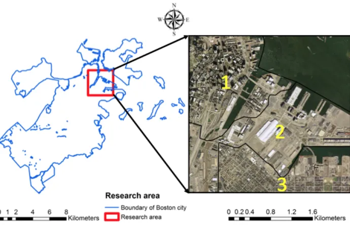
Chapter 3 shifts the subject to urban change detection. Urbanization has intensified across the globe at an unprecedented pace during the past several decades. Consequently, the demand for accurately acquiring urban building and building change information is expected to continue its increasing trend in the foreseeable future. LiDAR data contain full 3D information in the form of point clouds and are especially advantageous in detecting urban building changes. Previous research using LiDAR was significantly restricted by its rigid requirement of registration rate, rule-based removal of non-building objects, and high sensitivity due to comparison with mixed classes of points. In this research, we use a deep learning method to conduct a point-based urban building classification by adapting the PointSIFT algorithm to airborne LiDAR. Then we use an Euclidean-distance based clustering method to separate individual buildings and estimate building footprints. Finally, we infer building changes and classify change types by estimating the change of building volume and footprint from 3D alpha shapes, which is a generalization of the 3D convex hull and a subgraph of the Delaunay triangulation over a set of 3D points. Four types of changes including demolition, new construction, reduction, and expansion are extracted based on their different patterns. A reference dataset which is created by visual interpretation from both a multitemporal aerial photography and LiDAR data are used to separately evaluate the recall (completeness), precision (correctness), and F1 score of building classification and
change detection results. The estimated volumes in 2014 are also validated from 3D building survey data from the government data portal of Boston.
Chapter 4 investigates an important topic in hydrography-streamline detection. The accurate delineation of hydrological streamlines, which is one of the major forms of land surface water, is critically important in various scientific disciplines, such as the assessment of present and future water resources, climate models, agriculture suitability, river dynamics, wetland inventory, watershed analysis, surface water survey and management, flood mapping, and environmental monitoring. Traditional hydrological models generate streamlines solely based on topological information, which inevitably contain errors. For example, dried out drainage lines would always be falsely recognized as streamlines. Traditional methods also ignore the
information from the complex 3D environment of streamlines and surface reflectance
information, which would potentially be helpful to accurately delineate streamlines. In recent years, the availability of high accuracy LiDAR data provides us a promising method to capture both 3D information of the environment and also surface reflectance information of land cover. LiDAR sensor uses NIR light in the form of a pulsed laser to measure ranges (variable distances) to the ground and also reflectance information at multiple returns. These light pulses generate precise, three-dimensional information about the shape of the surface characteristics. In this research, multiple LiDAR features maps are generated, and we developed an attention U-net model for doing the streamline detection and we also tested several traditional machine learning methods as our baseline for comparison.
Chapter 5 focuses on the computational scalability of the workflow for land cover
classification using LiDAR and multitemporal Landsat imagery and expands the research area to 34 counties of southeast Illinois. Although LiDAR data contain rich information about 3D
characteristics of various landscape types, the 3D feature extraction of a large amount of LiDAR data are often challenging mainly due to the complexity of such data and computational
intensity. This research mainly tackles the computational challenges by utilizing cyberGIS-enabled cyberinfrastructure. To be specific, we utilize high throughput computing for LiDAR data preprocessing using 17 computing nodes (200+ CPU cores). Data reprojection and noise removal functions are applied in parallel for each tile of LiDAR. We also optimize the LiDAR sample points queries using spatial indexing in the process of training, validation, and prediction sample preparation. After that, we conduct data augmentation and voxelization in parallel for the data samples and use the GPU resource from Chameleon cloud service for a 3D CNN model training. In the classification stage, we optimize the RBF kernel calculation by using a GPU for the classification of seven land cover types. As the last step, we utilize a multi-GPU architecture to do model prediction over the research area to generate the final classified map.
Chapter 6 is the last chapter that summarizes the contributions of the dissertation, describes the limitations, and points out future work and potential research directions.
1.5 Synthesis and contribution
Most of current deep learning models in remote sensing data analysis are designed based on 2D learning or with limited expression of 3D information at a small scale. There are limited progress on 3D deep learning frameworks that are specifically designed for analyzing geospatial big data in 3D. The major contribution of this research is to develop and apply 3D deep learning frameworks to 3D geospatial big data in terms of landscape feature extraction and change detection. The primary goal of this research is to establish a cyberGIS-enabled deep learning framework to perform landscape feature extraction and classification using LiDAR data and
optical remote sensing data. The proposed methods in this framework not only pave a new way for understanding landscape patterns and dynamics in 3D, but also demonstrate its large-scale applications. The major conclusions from the four interrelated research investigations highlight the importance of advancing cyberGIS-enabled deep learning for mapping land cover patterns and dynamics using remote sensing big data.
1.6 Publications
Chapter 2: Xu, Z., Guan, K., Casler, N., Peng, B., & Wang, S. (2018). A 3D
convolutional neural network method for land cover classification using LiDAR and multi-temporal Landsat imagery. ISPRS journal of photogrammetry and remote sensing, 144, 423-434.
Chapter 4: Xu, Z., Guan, K., & Wang, S. (under review). Urban building extraction and change detection using multitemporal LiDAR data based on a deep learning and rule-based method. IEEE Journal of Selected Topics in Applied Earth Observations and Remote Sensing.
Chapter 5: Xu, Z., Wang, S., Stanislawski, L. V., Jiang Z., Jaroenchai, N., Sainju, A. M., Shavers, E., Usery E. L., Chen L., Li, Z., & Su, B. (under review). Hydrological streamline detection using a U-net model. Nature Machine Intelligence.
Rahil,S., Xu, Z., Sugumaran, R., Oliveira, S.(2016). Parallel Landscape Driven Data Reduction Spatial Interpolation Algorithm for Big LiDAR Data. ISPRS International Journal of Geo-Information, 5, no.6:97.
Xiao, C., Chen, N., Hu, C., Wang, K., Xu, Z., Cai, Y., Xu, L., Chen, Z., Gong, J. (2019). A spatiotemporal deep learning model for sea surface temperature field prediction using time-series satellite data. Environmental Modelling & Software, 104502.
Cienciala, P., Nelson, A. D., Haas, A. D., & Xu, Z.. (2020). Lateral geomorphic
connectivity in a fluvial landscape system: Unraveling the role of confinement, biogeomorphic interactions, and glacial legacies. Geomorphology, 107036.
Chen, L., Xu Z., Li H., Wang, S. (under review). Should we trust the deep neural network for remote sensing image classification? A Comprehensive Analysis. ISPRS Journal of
Photogrammetry and Remote Sensing.
Chen, L., Xu Z., Li H., Wang, S. (under review). DAPnet: A double attention
convolutional network for segmentation of point clouds. ISPRS Journal of Photogrammetry and Remote Sensing.
Lyu, F., Xu Z., Wang, S., Li Z., Ma, X., Wang, S. (under review). A Vector-Based Method for Drainage Network Analysis Based on LiDAR Data. Computers and Geosciences.
CHAPTER 2: A 3D CONVOLUTIONAL NEURAL NETWORK METHOD FOR LAND COVER CLASSIFICATION USING LIDAR AND MULTI-TEMPORAL LANDSAT
IMAGERY Abstract
The terrestrial landscape has complex three-dimensional (3D) features that are difficult to extract using traditional methods based on 2D representations. These methods often relegate such features to raster or metric-based (two-dimensional) representations based on Digital Surface Models (DSM) or Digital Elevation Models (DEM), and thus are not suitable for resolving morphological and intensity features for fine-scale land cover mapping.
Small-footprint LiDAR provides an ideal way for capturing these 3D features. This research develops a novel method of integrating airborne LiDAR derived features and multi-temporal Landsat images to classify land cover types. We tested our approach in Williamson County, Illinois, which has diverse and mixed landscape features. Specifically, our method applied a 3D
convolutional neural network (CNN) method to extract features from LiDAR point clouds by (1) creating an occupancy grid, an intensity grid at 1-meter resolution, and then (2) normalizing and incorporating data into the 3D CNN. The extracted features (e.g., morphological and intensity features) from the 3D CNN were finally combined with multi-temporal spectral data to enhance the performance of land cover classification based on a Support Vector Machine classifier. Visual interpretation from both hyper-resolution photos and point clouds was used for training and preparation of testing data. The classification results show that our method outperforms a traditional method by 2.65% (from 81.52% to 84.17%) when solely using LiDAR and 2.19% (from 90.20% to 92.57%) when combining all available images. We demonstrate that our
method can effectively extract LiDAR features and improve fine-scale land cover mapping through fusion of complementary types of remote sensing data.
2.1 Introduction and background
Land cover and land uses greatly impact various climatic and land surface processes. These processes, including energy balance, carbon and hydrological cycles, and land-atmosphere interactions, depend on the physical and/or biogeochemical properties (e.g., albedo, emissivity, photosynthetic capacity) of different land cover types (Foley et al., 2005; Brovkin et al., 2013; Bagley et al., 2014; Zhu and Woodcock, 2014; Costa et al., 2016). Land cover information has also been widely used by policy makers for land management, environmental stewardship, and risk and disease controls (Homer et al., 2015).
Satellite remote sensing has been widely used as an effective and efficient means to monitor land cover patterns at a large geographic extent. However, traditional remote sensing methods based on optical data (i.e. visible and near-infrared) are only suitable for capturing horizontally distributed features including shapes, structures, and areas. Because of the complexity of land cover types, Light Detection and Ranging (LiDAR) data becomes more frequently used to provide more information about land cover and enable the use of 3D characteristics of various landscape types to generate high quality land cover maps. Much research has been done in using geometric components of LiDAR data to improve land cover classifications. Many researchers used LiDAR derived information, including digital surface models (DSM), digital terrain models (DTM), and point density and spatial statistics calculated from LiDAR data for distinguishing land cover types. Various classification methods are also used when including LiDAR data, such as maximum likelihood algorithms (Bartels and Wei, 2006), object-oriented modeling (Brennan and
Webster, 2006; Carlberg et al., 2009), neural networks (Nguyen et al., 2005), SVMs (Lodha et al., 2006), and other machine learning algorithms (Charaniya et al., 2004; Zhu and Toutin, 2011; Chen et al., 2017). Extensive findings suggest that statistical features derived from intensity value of LiDAR are also helpful in distinguishing some classes that have little morphological variation (Brennan and Webster, 2006; Antonarakis et al., 2008; Bretar et al., 2008; Zhou, 2013; Morsy et al., 2016). More importantly, there has been an increasing interest in combining both optical data including multispectral imagery (Guo et al., 2011; Syed et al., 2005; Singh et al., 2012; Wulder et al., 2007; Lee and Jie, 2003), RGB imagery (Chen et al., 2009), high spatial resolution near-infrared imagery (Sasaki et al., 2012; Arroyo et al., 2010), hyperspectral imagery (Dalponte et al., 2008) and LiDAR data to achieve improved accuracy of land cover maps. In these processes, LiDAR derived metrics and spectral bands are combined and fit into various algorithms for classification. These algorithms include random forest (Guo et al., 2011), Support Vector Machines (SVMs) (Bretar et al., 2008; García-Gutiérrez et al., 2015), object-oriented classifiers (Syed et al., 2005; Sasaki et al., 2012; Arroyo, 2010; Chen et al., 2009), rule-based model (Huang et al., 2008), and structural and intensity surface models (Singh et al., 2012). While these analyses have provided key insights into high-resolution land cover mapping, they all conducted analysis based on traditional LiDAR metrics (e.g., variance, entropy, skewness, kurtosis), and there has been little work on using deep learning feature extraction framework to help understand and extract features at a much more complex and abstract level by using the full three-dimensional point cloud and intensity data that LiDAR collects.
During recent years, biologically inspired Convolutional Neural Networks (CNNs) have emerged and proven to be effective in various pattern recognition and object classification tasks (Krizhevsky et al., 2012; Razavian et al., 2014). During the training process, CNNs learn
hierarchical features, corresponding to different levels of abstraction. Novel architecture of CNNs have been widely acknowledged as the most successful deep learning approach, and used as dominant methods in many recognition and detection tasks (Krizhevsky et al., 2012;
Simonyan and Zisserman, 2015; Jia et al., 2014; Razavian et al., 2014; Oquab et al., 2014). However, the majority of CNNs are constructed based on 2D layers, which makes it difficult in solving classification tasks in 3D contexts. The recent development of 3D CNNs provides researchers new opportunities to solve classification problems in 3D space. Researchers can use different information for the third dimension. Temporal information is commonly used in video-based human action recognition (Ji et al., 2013). Some data have unique 3D information that is used for object recognition, such as tomography imagery with height information (Flitton et al., 2012), medical profile images from three dimensions as inputs (Kamnitsas et al., 2017). Hyper-spatial, multi-band imagery, which has different bands as the third dimension, is also used for 3D CNN model training in several land cover classification studies (Chen et al., 2016; Audebert et al., 2017; Ji et al., 2018). A depth image is another source for the third dimension that is combined with normal RGB images to form RGBD for 3D CNN applications including 3D object recognition (Socher et al., 2012; Gupta et al., 2014; Wu et al., 2015; Alexandre, 2016), and semantic segmentation (Hoft et al., 2014). The work by Prokhorov (2010) developed a 3D CNN with LiDAR data applied to a binary object classification problem. After that, Maturana and Scherer (2015a, 2015b) designed a generalized 3D CNN method called Voxnet for object classification using the full volumetric point cloud information from LiDAR, which was proven to be superior to other 3D CNNs. They also pointed out the future of using intensity attributes for classifying more complex scenes (Maturana and Scherer, 2015b). In addition, voxelization of intensity data is a solid way for data normalization (Reymann and Lacroix, 2015).
In this research, we have developed a novel method for complex feature learning from LiDAR data to improve land cover classification. The Voxnet architecture has several
advantages that make it suitable for our research problem. First, the architecture is able to learn local spatial filters useful to the classification task. In our case, we use activation maps from filters to encode structures such as planes and corners at different scales. Second, the hierarchy of more complex features can be extracted based on the stacking of multiple CNN layers over the entire feature space. Third, our new method is trained fully from the raw volumetric data based on the activations of each sub volume of data, where probabilities are finally calculated for class prediction. However, Voxnet is a 3D CNN classifier, which only allows the input of single type of data. Thus we adapt the architecture specifically to solve our problem for classification using both LiDAR and imagery data. During the training, the fully connected layer in the last epoch is removed and the last dense layer is extracted as the output. Then these features are combined with multitemporal spectral data for the final classification using a multi-class SVM classifier. The major contributions of this research are two-fold: (1) a novel method for land cover feature extraction by using full geometric and intensity information from LiDAR data, and (2) an effective data fusion model of using 3D features from LiDAR and multi-temporal images to achieve high accuracy in land cover classification.
2.2 Study area and dataset 2.2.1 Study area
Our study area includes the majority of Williamson County, Illinois, USA (Figure 2-1).
This area has 1,138 km2 with a population of 66,357. It has a mix of humid continental and
including tornadoes and winter storms. Summer is humid with warm temperature sometimes reaching 100 °F (38 °C). Fall is mild with heavy rainfall. Winter has periodic snow when the temperature reaches around 32 °F (0 °C). This area contains a complex composition and heterogeneous distribution of forest, shrub land, wetland, grassland and various types of agricultural land, water body, and developed land.
Figure 2-1. Research area (Williamson County, Illinois; Landsat 5 TM image: bands composition 5, 4, 3 and taken on July 22, 2011)
2.2.2 Dataset
Regarding the spectral data side, this study uses twelve cloud-free Landsat 5 surface reflectance scenes downloaded from the USGS Earth Explorer Data Portal
(https://earthexplorer.usgs.gov/). These images were separately acquired on August 20, August 27, September 5, September 12, September 21, October 7, October 14, October 30, 2010 and
January 2, April 17, June 4, July 22, 2011. Six TM bands (blue, green, red, near IR, and two mid IR bands) from each image are utilized to provide the spectral information for the classifications.
520 tiles of LiDAR data were flown from April 6-17, 2011 covering the research region and downloaded from the Illinois Geospatial Clearing House
(https://clearinghouse.isgs.illinois.edu). The data were collected by Federal Emergency
Management Agency and rectified by multiple companies to ensure both vertical and horizontal accuracy. The vertical accuracy is 8.53 cm RMSE and horizontal accuracy of 0.2 meter with a point spacing of 1.4 meters. The instrument collected up to 4 discrete returns per pulse, with intensity readings of 12-bit dynamic range per measurement, at around 1045nm. The delivered
data had an average density of 2 points per m2 and ranged from 1-5 points per m2 among
different tiles.
The Illinois Department of Transportation (IDOT) Orthophotography that was flown in April, 2011, using a Z/I Imaging Digital Mapping Camera (DMC) with RGB at a resolution of 1 feet, was downloaded from the Illinois Geospatial Clearing House
(https://clearinghouse.isgs.illinois.edu) and used as the source to generate reference data through visual interpretation. Because the twelve images, LiDAR, and reference source are all within a 12-month period, the land cover is assumed to be consistent and thus the same reference data can be used for classification of all images and LiDAR.
2.3 Methods
2.3.1 Method overview
The new method consists of data preparation, 3D CNN-based LiDAR feature extraction and classification. The feature extractor is adapted from Voxnet, which contains four types of
layers: convolutional, pooling, dropout and fully connected. The primary purpose of the convolutional layer is to extract features from original images. The convolutional process preserves the spatial relationship between pixels by learning image features using predefined multidirectional kernels to filter small squares of input data. The dropout layer is designed to randomly drop out neurons in order to avoid overfitting. The pooling layer conducts spatial down sampling by reducing the dimensionality of each feature map while retaining important
spatial information. The fully connected layer is a traditional multi-layer perceptron that uses a softmax function to produce categorical probability distribution of a certain number of classes to the output layer. The fully connected layer conducts different classification tasks based on these features and training labels. In our study, we revised Voxnet as a feature extractor by abandoning fully connected layers during the last training epoch. Also, the standard input of Voxnet is cubic
data volume. We instead use rectangular cuboid (30×30×50 m3), where the first and second
dimensions correspond to the resolution of the spectral data and the third dimension corresponds to height dimension. In the training process, we adjusted the batch size to fit our memory and set the maximum training epochs to 800.
2.3.2 Sampling design
In order to collect representative samples of each class in the population, it is important to keep the inclusion probability the same for each pixel (Xu et al., 2017). Thus, we selected 9000
pixels randomly on a 999×1282 fishnet grid (30 m) based on the Landsat imagery and overlaid
on the orthophotography. On-screen interpretation of both LiDAR and photography and
digitization are utilized to generate reference data. Finally, 8297 of them are useful and 703 are abandoned either because of cloud coverage or image registration errors. The general
interpretation principle is that a sample is assigned a class label if that class has a dominant coverage (>50%). One exception is that any sample contains more than 30% of developed type would be classified as developed to consider the connectivity of roads. Explicitly, we define herbaceous as dominant vegetation coverage lower than 1 meter; shrub as dominant vegetation coverage higher than or equal to 1 meter and lower than 5 meters; forest as dominant vegetation coverage higher than or equal to 5 meters. Both LiDAR and orthophotography were flown in April, which is the most humid season in the research area, so wetlands are defined as any vegetated area that is saturated with water. Among the 8297 samples, 70% (5808) are adopted as training data and 30% (2489) are adopted as testing for accuracy evaluation. Details of the reference data are listed in Table 2-1.
Table 2-1. Training and testing data number
2.3.3 Data preprocessing
Twelve multi-temporal land surface reflectance images are georeferenced with
orthophotography and reprojected from WGS84/UTM 16N to NAD83/UTM 16N. They are also cropped based on the boundary of Williamson County using ArcGIS 10.4 data management toolbox (ESRI, 2016). Six bands (blue, green, red, near IR, and two shortwave IR bands) from each image are extracted, and the normalized difference vegetation index (NDVI) (Carlson and Ripley, 1997) is calculated for each image using red and near-infrared bands of the TM imagery. Additionally, five texture-based statistics are calculated using grey level co-occurrence matrices (GLCMs) of each image. These layers are stacked as the spectral data for classification. The
texture features include contrast, dissimilarity, homogeneity, energy and correlation and their formulas are shown below (Chen et al., 1998).
𝐶𝑜𝑛𝑡𝑟𝑎𝑠𝑡 = ∑ ∑ (𝑖 − 𝑗)/ 0 𝑃2(𝑖, 𝑗) 4 (2.1) 𝐷𝑖𝑠𝑠𝑖𝑚𝑖𝑙𝑎𝑟𝑖𝑡𝑦 = ∑ ∑ 𝑃4 0 2(𝑖, 𝑗)|𝑖 − 𝑗| (2.2) 𝐻𝑜𝑚𝑜𝑔𝑒𝑛𝑒𝑖𝑡𝑦 = ∑ ∑ =>(4,0) ?@|4A0| 0 4 (2.3) 𝐸𝑛𝑒𝑟𝑔𝑦 = ∑ ∑ 𝑃2(𝑖, 𝑗)/ 0 4 (2.4) 𝐶𝑜𝑟𝑟𝑒𝑙𝑎𝑡𝑖𝑜𝑛 = ∑ ∑ [(4ADE)(0A DG) H(IEJ)(IGJ) ] 0 4 (2.5)
where Pd is the co-occurrence matrix in a rectangle neighborhood (7x7) of a center pixel, i is the
row number and j is the column number in Pd. σ2and µ are separately the variance and mean of a
row or column of values in Pd.
Point data abstraction library (Pdal), a C++ based open source point cloud processing library, is used for LiDAR data preprocessing. LiDAR data are initially reprojected from the State Plane Illinois East US feet (2011) to NAD83 UTM 16N to keep it consistent with spectral data. A statistics-based outlier filter was used to get rid of isolated noisy points including birds, powerlines, etc. We first calculated mean distance of each point to its twelve neighbors. Any point falls below or above two standard deviations of the mean distance of all the points in 3D space would be treated as an outlier and removed. The pipeline of LiDAR data preprocessing is shown in Figure 2-2 below.
2.3.4 Benchmark method
The benchmark method consists of the following three components: data preparation, 2D-CNN-based LiDAR feature extraction, and classification. Data preparation includes ground/non-ground classification, generation of feature maps from ground/non-ground/non-ground/non-ground returns, and LiDAR statistics calculation. In this process, the raw LiDAR data are reclassified into ground and non-ground classes using LAStools (Isenburg, 2011). Then non-ground/non-non-ground points are separately used to generate DSM, DEM, ground and non-ground intensity maps at a resolution of 1m using blast2dem function in LAStools (Isenburg, 2011). The four feature maps are then stacked and
feature map patches with the dimension of 32×32×4 are extracted for each sample. Five types of
LiDAR statistical features (kurtosis, variance, coefficient of variation, skewness, and entropy) are separately calculated from the elevation and intensity distribution of points of each sample. In the second stage, a 2D CNN model is constructed as shown in Figure 2-3. This model consists of three convolutional layers with 32 filters at the size of (3, 3) and a step of (1,1), three
maximum pooling layers with a step 2, a dropout layer with dropping rate of 0.45, a fully connected layer, and an output layer. The model is trained 800 epochs, and the last dense vector is extracted after the training is done. Different dimensions of dense vector (32, 64, and 128) are tested and 32 is finally selected because of its superiority. In the classification stage, the five types of statistical features are combined with the dense vector extracted from the 2D CNN model and LSR data for the final classification using a multi-class SVM classifier. The parameter tuning is conducted based on a three-level grid search and ten-fold cross-validation strategy. The best combination of parameters is used on the testing data for accuracy evaluation.
Figure 2-3. Flow chart of a 2D-CNN-based benchmark method
A standardized processing chain for DSM generation is utilized to map the above-ground height information in the study area using LAStools (Isenburg, 2011) and Pdal
(https://www.pdal.io). To avoid edge artifacts in the following image processing procedures, non-overlapping LiDAR tiles are retiled with a 60-meter buffer around each of them. First, LiDAR points are classified into ground points and non-ground points, and the digital terrain model is generated with the ground points using the triangular irregular network (TIN) (Isenburg et al., 2006). Raw LiDAR points are then height-normalized by subtracting the digital terrain model from the orthometric heights at the corresponding locations. Finally, DSM is generated at a resolution of 1m from the filtered points.
Table 2-2 shows the five types of LiDAR statistics that are used in the benchmark method. These statistical features are calculated separately from the elevation and intensity of LiDAR point cloud including variance, the coefficient of variation, kurtosis, skewness, entropy, that describes elevation and intensity characteristics of the point cloud. The entropy formula is specified below:
𝐸𝑛𝑡𝑟𝑜𝑝𝑦 = − MR4S?(𝑃(𝑖) ∗ log (𝑃(𝑖))) (2.6) where P(i) is the elevation or intensity value of point i.
In the classification stage, we use a radial basis function (RBF) kernel for SVM because of its superiority of mapping feature vector in high dimensional feature space and enable better class separability (Schölkopf and Smola, 2002). During training, two parameters are optimized: the penalty parameter, C, and the kernel width, s. C provides a trade-off between the margin among classes and the number of target objects rejected. Kernel width resolves the complexity of the delineation of margins between classes (Lo and Wang, 2012). A 2D grid search method is adopted three times to find the best parameter combination. The initial searching range is a
logarithmic grid from 10-5 to 105 with 1600 combinations. After using this first round of
optimization to narrow the potential value for C and s, another two rounds of searching in linear space each with 1600 combinations are used in secondary and tertiary searches to find the best parameter combination.
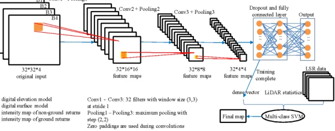
2.3.5 3D CNN-based multi-stage classification
The flowchart of the new method is shown in Figure 2-4. Data preparation includes data alignment of LiDAR tiles with Landsat pixels and LiDAR tiles augmentation to standardize LiDAR for feature learning. In the process of LiDAR feature extraction, voxelization is
is trained based on the two types of grids. After feature extraction, extracted features are combined with spectral data for the final classification using a multi-class SVM. The same parameter tuning and accuracy assessment strategy as the benchmark method is used. The only difference is that a majority vote of sample rotations is conducted as the final step to yield the classified map. The details of major steps are described below.
Figure 2-4. Flow chart of 3D CNN-based multi-stage classification
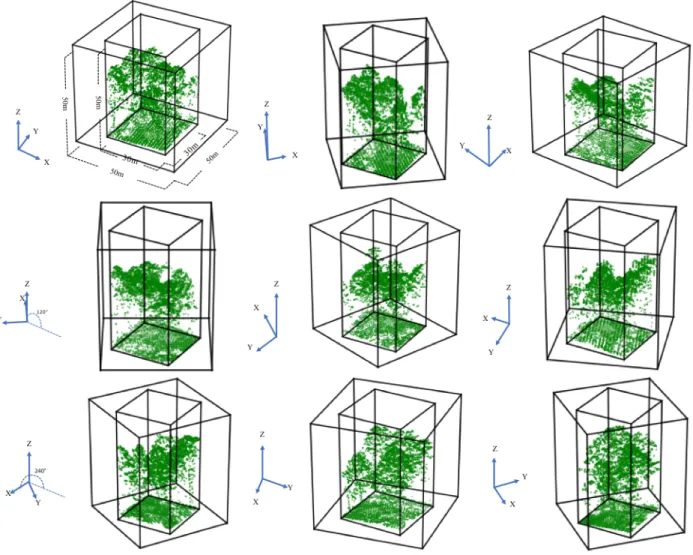
The same noise removal process is conducted for the new method to get rid of outlier points. After noise removal, data alignment is conducted by cropping LiDAR tiles corresponding to Landsat pixels. The point cloud cropping tool in the Pdal Library is used to extract points aligned with each Landsat pixel in the study area. In this process, boundary areas without LiDAR coverage are removed. To ensure the spatial invariant property (the ability to correctly classify samples wherever it appears in a defined space) and thus enhance the robustness of the model, data augmentation is done by rotating each training sample 9 angles around their z-axis. So for two neighboring samples, their rotation difference is 40 degrees (Figure 2-5). To avoid edge
point missing issues when rotating, we create 10-meter buffers for each sample in x and y direction and crop them using the sample mask after rotations.
After data augmentation, a grid size of 30×30×50 m3 is used to standardize each tile of
LiDAR at a resolution of 1 m3. This size is chosen to ensure a balance between data quality (1 –
5 points/m2) and computational intensity. The 1 m3 resolution does not lead to loss of useful
details since the land cover features of interest usually are larger than 1 m3. In 3D space of each
tile, x and y have the same dimension of 30 m that also equals to the size of its corresponding image pixel. The height dimension is chosen to be 50 m. Those tiles with points higher than 50 m are normalized to fit the grid. The bottom of a grid is set as the height of the lowest point within its LiDAR tile. In the model, we constructed two types of grids: occupancy and intensity grids. Figure 2-6 shows a voxelization example by constructing a grid of voxels (small unit cubes) overlaid with LiDAR points. Occupancy grid only counts the existence of LiDAR point
(1 or 0) within a 1 m3 voxel. This means no matter how many points falling within the unit, the
occupancy voxel always has the value 1 and the opposite has the value 0. An intensity grid is created by calculating the average intensity values of all the points falling within the voxel, and the average value is assigned to it. If there is no point in a voxel, its value is set to 0.
Figure 2-5. LiDAR sample rotations with 10-meter buffers in x and y (40 degrees each and totally nine directions counter clockwise)
Figure 2-6. Example of the data voxelization
The structure of the 3D Convolutional Neural Network (CNN) feature extractor is shown in Figure 2-7, adapted from the Voxnet developed by Maturana and Scherer for an object
classification task (Maturana and Scherer, 2015a, 2015b). The network contains two
convolutional layers, one pooling layer, three dropout layers and a fully connected layer. We change this network into a feature extractor by removing the fully connected layer during the last epoch of training and extract the last dense layer as output. We also adjust the input data format and a series of model parameters in order to serve our experimentation. In Figure 2-7, the input
layer accepts two fixed-size grids of x(32m)×y(32m)×z(52m) voxels and are created by adding
two 1m paddings to each dimension of origin grids (30m×30m×50m). The two convolutional
Layers (a, b, c) accept four-dimensional input volumes in which three of the dimensions are spatial, and the fourth contains the activation maps. These layers create c feature maps by
convolving the input with c learned filters of shape d×d×d×c, where d is the spatial dimension
spatial stride to reduce redundant spatial details. The first convolution layer uses 32 filters with a
window size of 5×5, a stride of 2 and produce activations maps with the dimension of 14×14×24.
Then the output is passed through a dropout layer with parameter 0.1. The second convolution
layer accepts these and produces activation maps with the dimension of 12×12×22. The pooling
Layer is used to down sample the input volume by a factor of m along the spatial dimensions by
replacing each m×m×m non-overlapping block of voxels with their maximum. In our case, the
dimension of output layer from pooling is 6×6×11. Then two dropout layers are used separately
with dropout rate of 0.3 and 0.4 to avoid overfitting. The fully connected layer comes the last to conduct a prediction on labels based on the combination of outputs from the previous layer (128 features).
Figure 2-7. Structure of 3D CNN feature extractor
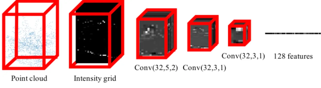
Figure 2-8 illustrates the 3D profile images of the intermediate layers generated from the network in a forest area. We can see that as the data goes through the different layers in the model, data volume reduces as tree crown features become more evident and synthesized, which is finally represented by 128 features.
Figure 2-8. Layers in the 3D convolutional feature extractor: the input layer (point cloud of a
forest sample); the intensity grid (52×32×32); the convolutional layer 1 (24×14×14); the
convolutional layer 2 (22×12×12); the pooling layer (11×6×6); the layer of 128 features.
To ensure the weights of neurons in the training process are updated timely, we divide the training data into five batches within every epoch. After each training on a single batch,
backpropagation is utilized to update the weights. Our model is trained 800 epochs, and the last dense layer is extracted as output instead of fitting into the fully connected layer. The reason we pick up this layer is that the 128 features are both qualitatively and quantitatively effective to aid in the classification. After feature learning, features extracted from occupancy and intensity grids are combined with spectral data for the final round of classification using SVM. Final results are achieved from a majority voting based on the votes from the nine rotation samples.
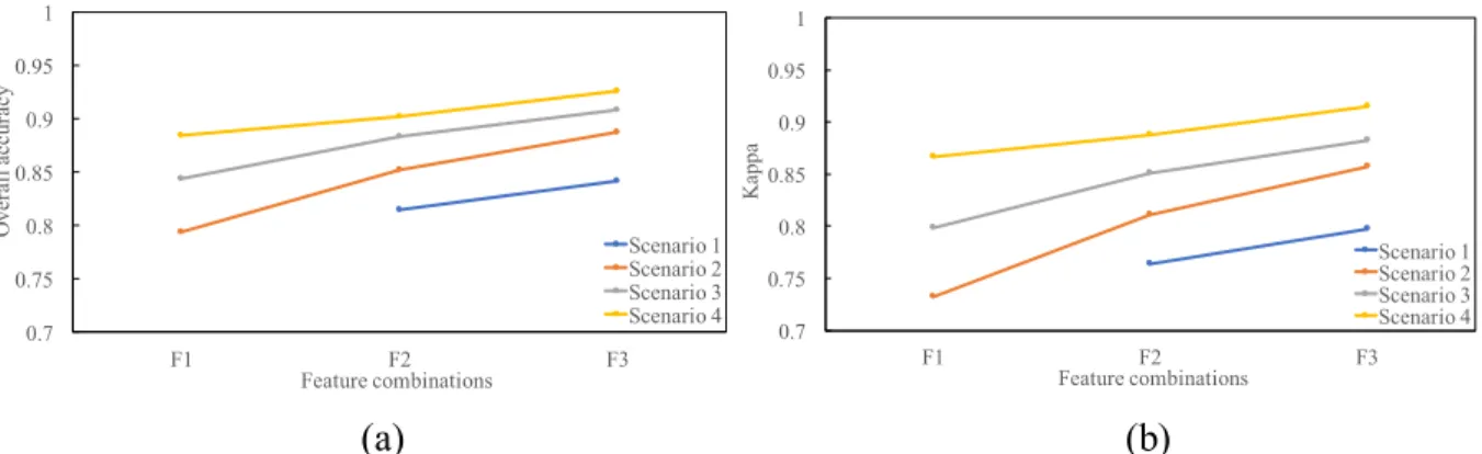
To compare the results when different numbers of images are included, four scenarios using solely LiDAR, single time image plus LiDAR, flush and senescence image pair plus LiDAR, and all images plus LiDAR are constructed. Both the benchmark method and our new model are tested, trained and evaluated using the same training, testing dataset and parameter tuning strategy with each scenario. The basic structures of these scenarios are listed in Table 2-3.